Ibm spss decision_trees

Note: Before using this information and the product it supports, read the general information
under Notices on p. 104.
This edition applies to IBM® SPSS® Statistics 20 and to all subsequent releases and modifications
until otherwise indicated in new editions.
Adobe product screenshot(s) reprinted with permission from Adobe Systems Incorporated.
Microsoft product screenshot(s) reprinted with permission from Microsoft Corporation.
Licensed Materials - Property of IBM
© Copyright IBM Corporation 1989, 2011.
U.S. Government Users Restricted Rights - Use, duplication or disclosure restricted by GSA ADP
Schedule Contract with IBM Corp.

Preface
IBM® SPSS® Statistics is a comprehensive system for analyzing data. The Decision Trees
optional add-on module provides the additional analytic techniques described in this manual.
The Decision Trees add-on module must be used with the SPSS Statistics Core system and is
completely integrated into that system.
About IBM Business Analytics
IBM Business Analytics software delivers complete, consistent and accurate information that
decision-makers trust to improve business performance. A comprehensive portfolio of business
intelligence, predictive analytics, financial performance and strategy management, and analytic
applications provides clear, immediate and actionable insights into current performance and the
ability to predict future outcomes. Combined with rich industry solutions, proven practices and
professional services, organizations of every size can drive the highest productivity, confidently
automate decisions and deliver better results.
As part of this portfolio, IBM SPSS Predictive Analytics software helps organizations predict
future events and proactively act upon that insight to drive better business outcomes. Commercial,
government and academic customers worldwide rely on IBM SPSS technology as a competitive
advantage in attracting, retaining and growing customers, while reducing fraud and mitigating
risk. By incorporating IBM SPSS software into their daily operations, organizations become
predictive enterprises – able to direct and automate decisions to meet business goals and achieve
measurable competitive advantage. For further information or to reach a representative visit
http://www.ibm.com/spss.
Technical support
Technical support is available to maintenance customers. Customers may contact Technical
Support for assistance in using IBM Corp. products or for installation help for one of the
supported hardware environments. To reach Technical Support, see the IBM Corp. web site
at http://www.ibm.com/support. Be prepared to identify yourself, your organization, and your
support agreement when requesting assistance.
Technical Support for Students
If you’re a student using a student, academic or grad pack version of any IBM
SPSS software product, please see our special online Solutions for Education
(http://www.ibm.com/spss/rd/students/) pages for students. If you’re a student using a
university-supplied copy of the IBM SPSS software, please contact the IBM SPSS product
coordinator at your university.
Customer Service
If you have any questions concerning your shipment or account, contact your local office. Please
have your serial number ready for identification.
© Copyright IBM Corporation 1989, 2011. iii

Training Seminars
IBM Corp. provides both public and onsite training seminars. All seminars feature hands-on
workshops. Seminars will be offered in major cities on a regular basis. For more information on
these seminars, go to http://www.ibm.com/software/analytics/spss/training.
Additional Publications
The SPSS Statistics: Guide to Data Analysis, SPSS Statistics: Statistical Procedures Companion,
and SPSS Statistics: Advanced Statistical Procedures Companion, written by Marija Norušis and
published by Prentice Hall, are available as suggested supplemental material. These publications
cover statistical procedures in the SPSS Statistics Base module, Advanced Statistics module
and Regression module. Whether you are just getting starting in data analysis or are ready for
advanced applications, these books will help you make best use of the capabilities found within
the IBM® SPSS® Statistics offering. For additional information including publication contents
and sample chapters, please see the author’s website: http://www.norusis.com
iv

Contents
Part I: User’s Guide
1 Creating Decision Trees 1
Selecting Categories . . . . . . . . . . . . . . . . . . . . . . . . . . . . . . . . . . . . . . . . . . . . . . . . . . . . . . . . . . 6
Validation . . . . . . . . . . . . . . . . . . . . . . . . . . . . . . . . . . . . . . . . . . . . . . . . . . . . . . . . . . . . . . . . . . . 7
Tree-Growing Criteria . . . . . . . . . . . . . . . . . . . . . . . . . . . . . . . . . . . . . . . . . . . . . . . . . . . . . . . . . . 8
Growth Limits . . . . . . . . . . . . . . . . . . . . . . . . . . . . . . . . . . . . . . . . . . . . . . . . . . . . . . . . . . . . 9
CHAID Criteria . . . . . . . . . . . . . . . . . . . . . . . . . . . . . . . . . . . . . . . . . . . . . . . . . . . . . . . . . . . . 10
CRT Criteria . . . . . . . . . . . . . . . . . . . . . . . . . . . . . . . . . . . . . . . . . . . . . . . . . . . . . . . . . . . . . . 12
QUEST Criteria. . . . . . . . . . . . . . . . . . . . . . . . . . . . . . . . . . . . . . . . . . . . . . . . . . . . . . . . . . . . 13
Pruning Trees . . . . . . . . . . . . . . . . . . . . . . . . . . . . . . . . . . . . . . . . . . . . . . . . . . . . . . . . . . . . 14
Surrogates . . . . . . . . . . . . . . . . . . . . . . . . . . . . . . . . . . . . . . . . . . . . . . . . . . . . . . . . . . . . . . 15
Options. . . . . . . . . . . . . . . . . . . . . . . . . . . . . . . . . . . . . . . . . . . . . . . . . . . . . . . . . . . . . . . . . . . . . 15
Misclassification Costs . . . . . . . . . . . . . . . . . . . . . . . . . . . . . . . . . . . . . . . . . . . . . . . . . . . . . 16
Profits . . . . . . . . . . . . . . . . . . . . . . . . . . . . . . . . . . . . . . . . . . . . . . . . . . . . . . . . . . . . . . . . . . 17
Prior Probabilities . . . . . . . . . . . . . . . . . . . . . . . . . . . . . . . . . . . . . . . . . . . . . . . . . . . . . . . . . 18
Scores. . . . . . . . . . . . . . . . . . . . . . . . . . . . . . . . . . . . . . . . . . . . . . . . . . . . . . . . . . . . . . . . . . 20
Missing Values . . . . . . . . . . . . . . . . . . . . . . . . . . . . . . . . . . . . . . . . . . . . . . . . . . . . . . . . . . . 21
Saving Model Information. . . . . . . . . . . . . . . . . . . . . . . . . . . . . . . . . . . . . . . . . . . . . . . . . . . . . . . 22
Output . . . . . . . . . . . . . . . . . . . . . . . . . . . . . . . . . . . . . . . . . . . . . . . . . . . . . . . . . . . . . . . . . . . . . 23
Tree Display. . . . . . . . . . . . . . . . . . . . . . . . . . . . . . . . . . . . . . . . . . . . . . . . . . . . . . . . . . . . . . 24
Statistics . . . . . . . . . . . . . . . . . . . . . . . . . . . . . . . . . . . . . . . . . . . . . . . . . . . . . . . . . . . . . . . . 26
Charts . . . . . . . . . . . . . . . . . . . . . . . . . . . . . . . . . . . . . . . . . . . . . . . . . . . . . . . . . . . . . . . . . . 29
Selection and Scoring Rules . . . . . . . . . . . . . . . . . . . . . . . . . . . . . . . . . . . . . . . . . . . . . . . . . 35
2 Tree Editor 37
Working with Large Trees . . . . . . . . . . . . . . . . . . . . . . . . . . . . . . . . . . . . . . . . . . . . . . . . . . . . . . . 38
Tree Map. . . . . . . . . . . . . . . . . . . . . . . . . . . . . . . . . . . . . . . . . . . . . . . . . . . . . . . . . . . . . . . . 39
Scaling the Tree Display . . . . . . . . . . . . . . . . . . . . . . . . . . . . . . . . . . . . . . . . . . . . . . . . . . . . 39
Node Summary Window . . . . . . . . . . . . . . . . . . . . . . . . . . . . . . . . . . . . . . . . . . . . . . . . . . . . 40
Controlling Information Displayed in the Tree . . . . . . . . . . . . . . . . . . . . . . . . . . . . . . . . . . . . . . . . 41
Changing Tree Colors and Text Fonts. . . . . . . . . . . . . . . . . . . . . . . . . . . . . . . . . . . . . . . . . . . . . . . 42
Case Selection and Scoring Rules . . . . . . . . . . . . . . . . . . . . . . . . . . . . . . . . . . . . . . . . . . . . . . . . 44
Filtering Cases. . . . . . . . . . . . . . . . . . . . . . . . . . . . . . . . . . . . . . . . . . . . . . . . . . . . . . . . . . . . 44
Saving Selection and Scoring Rules. . . . . . . . . . . . . . . . . . . . . . . . . . . . . . . . . . . . . . . . . . . . 45
v

Part II: Examples
3 Data assumptions and requirements 48
Effects of measurement level on tree models . . . . . . . . . . . . . . . . . . . . . . . . . . . . . . . . . . . . . . . . 48
Permanently assigning measurement level . . . . . . . . . . . . . . . . . . . . . . . . . . . . . . . . . . . . . . 51
Variables with an unknown measurement level . . . . . . . . . . . . . . . . . . . . . . . . . . . . . . . . . . . 52
Effects of value labels on tree models. . . . . . . . . . . . . . . . . . . . . . . . . . . . . . . . . . . . . . . . . . . . . . 52
Assigning value labels to all values . . . . . . . . . . . . . . . . . . . . . . . . . . . . . . . . . . . . . . . . . . . . 54
4 Using Decision Trees to Evaluate Credit Risk 55
Creating the Model. . . . . . . . . . . . . . . . . . . . . . . . . . . . . . . . . . . . . . . . . . . . . . . . . . . . . . . . . . . . 55
Building the CHAID Tree Model . . . . . . . . . . . . . . . . . . . . . . . . . . . . . . . . . . . . . . . . . . . . . . . 55
Selecting Target Categories. . . . . . . . . . . . . . . . . . . . . . . . . . . . . . . . . . . . . . . . . . . . . . . . . . 56
Specifying Tree Growing Criteria . . . . . . . . . . . . . . . . . . . . . . . . . . . . . . . . . . . . . . . . . . . . . . 57
Selecting Additional Output . . . . . . . . . . . . . . . . . . . . . . . . . . . . . . . . . . . . . . . . . . . . . . . . . . 58
Saving Predicted Values . . . . . . . . . . . . . . . . . . . . . . . . . . . . . . . . . . . . . . . . . . . . . . . . . . . . 60
Evaluating the Model . . . . . . . . . . . . . . . . . . . . . . . . . . . . . . . . . . . . . . . . . . . . . . . . . . . . . . . . . . 61
Model Summary Table . . . . . . . . . . . . . . . . . . . . . . . . . . . . . . . . . . . . . . . . . . . . . . . . . . . . . . 62
Tree Diagram. . . . . . . . . . . . . . . . . . . . . . . . . . . . . . . . . . . . . . . . . . . . . . . . . . . . . . . . . . . . . 63
Tree Table . . . . . . . . . . . . . . . . . . . . . . . . . . . . . . . . . . . . . . . . . . . . . . . . . . . . . . . . . . . . . . . 64
Gains for Nodes. . . . . . . . . . . . . . . . . . . . . . . . . . . . . . . . . . . . . . . . . . . . . . . . . . . . . . . . . . . 65
Gains Chart . . . . . . . . . . . . . . . . . . . . . . . . . . . . . . . . . . . . . . . . . . . . . . . . . . . . . . . . . . . . . . 66
Index Chart . . . . . . . . . . . . . . . . . . . . . . . . . . . . . . . . . . . . . . . . . . . . . . . . . . . . . . . . . . . . . . 66
Risk Estimate and Classification. . . . . . . . . . . . . . . . . . . . . . . . . . . . . . . . . . . . . . . . . . . . . . . 67
Predicted Values . . . . . . . . . . . . . . . . . . . . . . . . . . . . . . . . . . . . . . . . . . . . . . . . . . . . . . . . . . 68
Refining the Model . . . . . . . . . . . . . . . . . . . . . . . . . . . . . . . . . . . . . . . . . . . . . . . . . . . . . . . . . . . . 69
Selecting Cases in Nodes . . . . . . . . . . . . . . . . . . . . . . . . . . . . . . . . . . . . . . . . . . . . . . . . . . . 69
Examining the Selected Cases . . . . . . . . . . . . . . . . . . . . . . . . . . . . . . . . . . . . . . . . . . . . . . . . 70
Assigning Costs to Outcomes. . . . . . . . . . . . . . . . . . . . . . . . . . . . . . . . . . . . . . . . . . . . . . . . . 72
Summary . . . . . . . . . . . . . . . . . . . . . . . . . . . . . . . . . . . . . . . . . . . . . . . . . . . . . . . . . . . . . . . . . . . 76
5 Building a Scoring Model 77
Building the Model . . . . . . . . . . . . . . . . . . . . . . . . . . . . . . . . . . . . . . . . . . . . . . . . . . . . . . . . . . . . 77
Evaluating the Model . . . . . . . . . . . . . . . . . . . . . . . . . . . . . . . . . . . . . . . . . . . . . . . . . . . . . . . . . . 78
Model Summary . . . . . . . . . . . . . . . . . . . . . . . . . . . . . . . . . . . . . . . . . . . . . . . . . . . . . . . . . . 79
vi

Tree Model Diagram . . . . . . . . . . . . . . . . . . . . . . . . . . . . . . . . . . . . . . . . . . . . . . . . . . . . . . . 80
Risk Estimate. . . . . . . . . . . . . . . . . . . . . . . . . . . . . . . . . . . . . . . . . . . . . . . . . . . . . . . . . . . . . 81
Applying the Model to Another Data File. . . . . . . . . . . . . . . . . . . . . . . . . . . . . . . . . . . . . . . . . . . . 82
Summary . . . . . . . . . . . . . . . . . . . . . . . . . . . . . . . . . . . . . . . . . . . . . . . . . . . . . . . . . . . . . . . . . . . 85
6 Missing Values in Tree Models 86
Missing Values with CHAID . . . . . . . . . . . . . . . . . . . . . . . . . . . . . . . . . . . . . . . . . . . . . . . . . . . . . 86
CHAID Results . . . . . . . . . . . . . . . . . . . . . . . . . . . . . . . . . . . . . . . . . . . . . . . . . . . . . . . . . . . . 88
Missing Values with CRT. . . . . . . . . . . . . . . . . . . . . . . . . . . . . . . . . . . . . . . . . . . . . . . . . . . . . . . . 89
CRT Results . . . . . . . . . . . . . . . . . . . . . . . . . . . . . . . . . . . . . . . . . . . . . . . . . . . . . . . . . . . . . . 92
Summary . . . . . . . . . . . . . . . . . . . . . . . . . . . . . . . . . . . . . . . . . . . . . . . . . . . . . . . . . . . . . . . . . . . 94
Appendices
A Sample Files 95
B Notices 104
Index 107
vii

Chapter
1
Creating Decision Trees
Figure 1-1
Decision tree
The Decision Tree procedure creates a tree-based classification model. It classifies cases into
groups or predicts values of a dependent (target) variable based on values of independent
(predictor) variables. The procedure provides validation tools for exploratory and confirmatory
classification analysis.
The procedure can be used for:
Segmentation. Identify persons who are likely to be members of a particular group.
Stratification. Assign cases into one of several categories, such as high-, medium-, and low-risk
groups.
Prediction. Create rules and use them to predict future events, such as the likelihood that someone
will default on a loan or the potential resale value of a vehicle or home.
Data reduction and variable screening. Select a useful subset of predictors from a large set of
variables for use in building a formal parametric model.
© Copyright IBM Corporation 1989, 2011. 1

2
Chapter 1
Interaction identification. Identify relationships that pertain only to specific subgroups and specify
these in a formal parametric model.
Category merging and discretizing continuous variables. Recode group predictor categories and
continuous variables with minimal loss of information.
Example. A bank wants to categorize credit applicants according to whether or not they represent
a reasonable credit risk. Based on various factors, including the known credit ratings of past
customers, you can build a model to predict if future customers are likely to default on their loans.
A tree-based analysis provides some attractive features:
 It allows you to identify homogeneous groups with high or low risk.
 It makes it easy to construct rules for making predictions about individual cases.
Data Considerations
Data. The dependent and independent variables can be:
 Nominal. A variable can be treated as nominal when its values represent categories with no
intrinsic ranking (for example, the department of the company in which an employee works).
Examples of nominal variables include region, zip code, and religious affiliation.
 Ordinal. A variable can be treated as ordinal when its values represent categories with some
intrinsic ranking (for example, levels of service satisfaction from highly dissatisfied to
highly satisfied). Examples of ordinal variables include attitude scores representing degree
of satisfaction or confidence and preference rating scores.
 Scale. A variable can be treated as scale (continuous) when its values represent ordered
categories with a meaningful metric, so that distance comparisons between values are
appropriate. Examples of scale variables include age in years and income in thousands of
dollars.
Frequency weights If weighting is in effect, fractional weights are rounded to the closest integer;
so, cases with a weight value of less than 0.5 are assigned a weight of 0 and are therefore excluded
from the analysis.
Assumptions. This procedure assumes that the appropriate measurement level has been assigned
to all analysis variables, and some features assume that all values of the dependent variable
included in the analysis have defined value labels.
 Measurement level. Measurement level affects the tree computations; so, all variables should
be assigned the appropriate measurement level. By default, numeric variables are assumed to
be scale and string variables are assumed to be nominal, which may not accurately reflect

3
the true measurement level. An icon next to each variable in the variable list identifies the
variable type.
Scale
Nominal
Ordinal
You can temporarily change the measurement level for a variable by right-clicking the variable in
the source variable list and selecting a measurement level from the context menu.
 Value labels. The dialog box interface for this procedure assumes that either all nonmissing
values of a categorical (nominal, ordinal) dependent variable have defined value labels or
none of them do. Some features are not available unless at least two nonmissing values
of the categorical dependent variable have value labels. If at least two nonmissing values
have defined value labels, any cases with other values that do not have value labels will be
excluded from the analysis.
To Obtain Decision Trees
E From the menus choose:
Analyze > Classify > Tree...
Figure 1-2
Decision Tree dialog box
E Select a dependent variable.

4
Chapter 1
E Select one or more independent variables.
E Select a growing method.
Optionally, you can:
 Change the measurement level for any variable in the source list.
 Force the first variable in the independent variables list into the model as the first split variable.
 Select an influence variable that defines how much influence a case has on the tree-growing
process. Cases with lower influence values have less influence; cases with higher values have
more. Influence variable values must be positive.
 Validate the tree.
 Customize the tree-growing criteria.
 Save terminal node numbers, predicted values, and predicted probabilities as variables.
 Save the model in XML (PMML) format.
Fields with Unknown Measurement Level
The Measurement Level alert is displayed when the measurement level for one or more variables
(fields) in the dataset is unknown. Since measurement level affects the computation of results for
this procedure, all variables must have a defined measurement level.
Figure 1-3
Measurement level alert
 Scan Data. Reads the data in the active dataset and assigns default measurement level to
any fields with a currently unknown measurement level. If the dataset is large, that may
take some time.
 Assign Manually. Opens a dialog that lists all fields with an unknown measurement level.
You can use this dialog to assign measurement level to those fields. You can also assign
measurement level in Variable View of the Data Editor.
Since measurement level is important for this procedure, you cannot access the dialog to run this
procedure until all fields have a defined measurement level.
Changing Measurement Level
E Right-click the variable in the source list.

5
E Select a measurement level from the pop-up context menu.
This changes the measurement level temporarily for use in the Decision Tree procedure.
Growing Methods
The available growing methods are:
CHAID. Chi-squared Automatic Interaction Detection. At each step, CHAID chooses the
independent (predictor) variable that has the strongest interaction with the dependent variable.
Categories of each predictor are merged if they are not significantly different with respect to the
dependent variable.
Exhaustive CHAID. A modification of CHAID that examines all possible splits for each predictor.
CRT. Classification and Regression Trees. CRT splits the data into segments that are as
homogeneous as possible with respect to the dependent variable. A terminal node in which all
cases have the same value for the dependent variable is a homogeneous, "pure" node.
QUEST. Quick, Unbiased, Efficient Statistical Tree. A method that is fast and avoids other
methods’ bias in favor of predictors with many categories. QUEST can be specified only if
the dependent variable is nominal.
There are benefits and limitations with each method, including:
CHAID* CRT QUEST
Chi-square-based** X
Surrogate independent (predictor)
variables
X X
Tree pruning X X
Multiway node splitting X
Binary node splitting X X
Influence variables X X
Prior probabilities X X
Misclassification costs X X X
Fast calculation X X
*Includes Exhaustive CHAID.
**QUEST also uses a chi-square measure for nominal independent variables.

6
Chapter 1
Selecting Categories
Figure 1-4
Categories dialog box
For categorical (nominal, ordinal) dependent variables, you can:
 Control which categories are included in the analysis.
 Identify the target categories of interest.
Including/Excluding Categories
You can limit the analysis to specific categories of the dependent variable.
 Cases with values of the dependent variable in the Exclude list are not included in the analysis.
 For nominal dependent variables, you can also include user-missing categories in the analysis.
(By default, user-missing categories are displayed in the Exclude list.)
Target Categories
Selected (checked) categories are treated as the categories of primary interest in the analysis. For
example, if you are primarily interested in identifying those individuals most likely to default on a
loan, you might select the “bad” credit-rating category as the target category.
 There is no default target category. If no category is selected, some classification rule options
and gains-related output are not available.
 If multiple categories are selected, separate gains tables and charts are produced for each
target category.
 Designating one or more categories as target categories has no effect on the tree model, risk
estimate, or misclassification results.

7
Categories and Value Labels
This dialog box requires defined value labels for the dependent variable. It is not available unless
at least two values of the categorical dependent variable have defined value labels.
To Include/Exclude Categories and Select Target Categories
E In the main Decision Tree dialog box, select a categorical (nominal, ordinal) dependent variable
with two or more defined value labels.
E Click Categories.
Validation
Figure 1-5
Validation dialog box
Validation allows you to assess how well your tree structure generalizes to a larger population.
Two validation methods are available: crossvalidation and split-sample validation.
Crossvalidation
Crossvalidation divides the sample into a number of subsamples, or folds. Tree models are then
generated, excluding the data from each subsample in turn. The first tree is based on all of the
cases except those in the first sample fold, the second tree is based on all of the cases except those

8
Chapter 1
in the second sample fold, and so on. For each tree, misclassification risk is estimated by applying
the tree to the subsample excluded in generating it.
 You can specify a maximum of 25 sample folds. The higher the value, the fewer the number
of cases excluded for each tree model.
 Crossvalidation produces a single, final tree model. The crossvalidated risk estimate for the
final tree is calculated as the average of the risks for all of the trees.
Split-Sample Validation
With split-sample validation, the model is generated using a training sample and tested on a
hold-out sample.
 You can specify a training sample size, expressed as a percentage of the total sample size, or a
variable that splits the sample into training and testing samples.
 If you use a variable to define training and testing samples, cases with a value of 1 for the
variable are assigned to the training sample, and all other cases are assigned to the testing
sample. The variable cannot be the dependent variable, weight variable, influence variable,
or a forced independent variable.
 You can display results for both the training and testing samples or just the testing sample.
 Split-sample validation should be used with caution on small data files (data files with a small
number of cases). Small training sample sizes may yield poor models, since there may not be
enough cases in some categories to adequately grow the tree.
Tree-Growing Criteria
The available growing criteria may depend on the growing method, level of measurement of the
dependent variable, or a combination of the two.

9
Growth Limits
Figure 1-6
Criteria dialog box, Growth Limits tab
The Growth Limits tab allows you to limit the number of levels in the tree and control the
minimum number of cases for parent and child nodes.
Maximum Tree Depth. Controls the maximum number of levels of growth beneath the root node.
The Automatic setting limits the tree to three levels beneath the root node for the CHAID and
Exhaustive CHAID methods and five levels for the CRT and QUEST methods.
Minimum Number of Cases. Controls the minimum numbers of cases for nodes. Nodes that do not
satisfy these criteria will not be split.
 Increasing the minimum values tends to produce trees with fewer nodes.
 Decreasing the minimum values produces trees with more nodes.
For data files with a small number of cases, the default values of 100 cases for parent nodes and
50 cases for child nodes may sometimes result in trees with no nodes below the root node; in this
case, lowering the minimum values may produce more useful results.

10
Chapter 1
CHAID Criteria
Figure 1-7
Criteria dialog box, CHAID tab
For the CHAID and Exhaustive CHAID methods, you can control:
Significance Level. You can control the significance value for splitting nodes and merging
categories. For both criteria, the default significance level is 0.05.
 For splitting nodes, the value must be greater than 0 and less than 1. Lower values tend to
produce trees with fewer nodes.
 For merging categories, the value must be greater than 0 and less than or equal to 1. To
prevent merging of categories, specify a value of 1. For a scale independent variable, this
means that the number of categories for the variable in the final tree is the specified number of
intervals (the default is 10). For more information, see the topic Scale Intervals for CHAID
Analysis on p. 11.
Chi-Square Statistic. For ordinal dependent variables, chi-square for determining node splitting
and category merging is calculated using the likelihood-ratio method. For nominal dependent
variables, you can select the method:
 Pearson. This method provides faster calculations but should be used with caution on small
samples. This is the default method.
 Likelihood ratio. This method is more robust that Pearson but takes longer to calculate. For
small samples, this is the preferred method.

11
Model Estimation. For nominal and ordinal dependent variables, you can specify:
 Maximum number of iterations. The default is 100. If the tree stops growing because the
maximum number of iterations has been reached, you may want to increase the maximum or
change one or more of the other criteria that control tree growth.
 Minimum change in expected cell frequencies. The value must be greater than 0 and less than
1. The default is 0.05. Lower values tend to produce trees with fewer nodes.
Adjust significance values using Bonferroni method. For multiple comparisons, significance values
for merging and splitting criteria are adjusted using the Bonferroni method. This is the default.
Allow resplitting of merged categories within a node. Unless you explicitly prevent category
merging, the procedure will attempt to merge independent (predictor) variable categories together
to produce the simplest tree that describes the model. This option allows the procedure to resplit
merged categories if that provides a better solution.
Scale Intervals for CHAID Analysis
Figure 1-8
Criteria dialog box, Intervals tab
In CHAID analysis, scale independent (predictor) variables are always banded into discrete groups
(for example, 0–10, 11–20, 21–30, etc.) prior to analysis. You can control the initial/maximum
number of groups (although the procedure may merge contiguous groups after the initial split):
 Fixed number. All scale independent variables are initially banded into the same number of
groups. The default is 10.
 Custom. Each scale independent variable is initially banded into the number of groups
specified for that variable.

12
Chapter 1
To Specify Intervals for Scale Independent Variables
E In the main Decision Tree dialog box, select one or more scale independent variables.
E For the growing method, select CHAID or Exhaustive CHAID.
E Click Criteria.
E Click the Intervals tab.
In CRT and QUEST analysis, all splits are binary and scale and ordinal independent variables
are handled the same way; so, you cannot specify a number of intervals for scale independent
variables.
CRT Criteria
Figure 1-9
Criteria dialog box, CRT tab
The CRT growing method attempts to maximize within-node homogeneity. The extent to which a
node does not represent a homogenous subset of cases is an indication of impurity. For example,
a terminal node in which all cases have the same value for the dependent variable is a homogenous
node that requires no further splitting because it is “pure.”
You can select the method used to measure impurity and the minimum decrease in impurity
required to split nodes.
Impurity Measure. For scale dependent variables, the least-squared deviation (LSD) measure of
impurity is used. It is computed as the within-node variance, adjusted for any frequency weights
or influence values.

13
For categorical (nominal, ordinal) dependent variables, you can select the impurity measure:
 Gini. Splits are found that maximize the homogeneity of child nodes with respect to the
value of the dependent variable. Gini is based on squared probabilities of membership for
each category of the dependent variable. It reaches its minimum (zero) when all cases in a
node fall into a single category. This is the default measure.
 Twoing. Categories of the dependent variable are grouped into two subclasses. Splits are found
that best separate the two groups.
 Ordered twoing. Similar to twoing except that only adjacent categories can be grouped. This
measure is available only for ordinal dependent variables.
Minimum change in improvement. This is the minimum decrease in impurity required to split a
node. The default is 0.0001. Higher values tend to produce trees with fewer nodes.
QUEST Criteria
Figure 1-10
Criteria dialog box, QUEST tab
For the QUEST method, you can specify the significance level for splitting nodes. An independent
variable cannot be used to split nodes unless the significance level is less than or equal to the
specified value. The value must be greater than 0 and less than 1. The default is 0.05. Smaller
values will tend to exclude more independent variables from the final model.
To Specify QUEST Criteria
E In the main Decision Tree dialog box, select a nominal dependent variable.
E For the growing method, select QUEST.
E Click Criteria.

14
Chapter 1
E Click the QUEST tab.
Pruning Trees
Figure 1-11
Criteria dialog box, Pruning tab
With the CRT and QUEST methods, you can avoid overfitting the model by pruning the tree:
the tree is grown until stopping criteria are met, and then it is trimmed automatically to the
smallest subtree based on the specified maximum difference in risk. The risk value is expressed
in standard errors. The default is 1. The value must be non-negative. To obtain the subtree
with the minimum risk, specify 0.
Pruning versus Hiding Nodes
When you create a pruned tree, any nodes pruned from the tree are not available in the final
tree. You can interactively hide and show selected child nodes in the final tree, but you cannot
show nodes that were pruned in the tree creation process. For more information, see the topic
Tree Editor in Chapter 2 on p. 37.

15
Surrogates
Figure 1-12
Criteria dialog box, Surrogates tab
CRT and QUEST can use surrogates for independent (predictor) variables. For cases in which the
value for that variable is missing, other independent variables having high associations with the
original variable are used for classification. These alternative predictors are called surrogates. You
can specify the maximum number of surrogates to use in the model.
 By default, the maximum number of surrogates is one less than the number of independent
variables. In other words, for each independent variable, all other independent variables
may be used as surrogates.
 If you don’t want the model to use surrogates, specify 0 for the number of surrogates.
Options
Available options may depend on the growing method, the level of measurement of the dependent
variable, and/or the existence of defined value labels for values of the dependent variable.

16
Chapter 1
Misclassification Costs
Figure 1-13
Options dialog box, Misclassification Costs tab
For categorical (nominal, ordinal) dependent variables, misclassification costs allow you to include
information about the relative penalty associated with incorrect classification. For example:
 The cost of denying credit to a creditworthy customer is likely to be different from the cost of
extending credit to a customer who then defaults on the loan.
 The cost of misclassifying an individual with a high risk of heart disease as low risk is
probably much higher than the cost of misclassifying a low-risk individual as high-risk.
 The cost of sending a mass mailing to someone who isn’t likely to respond is probably fairly
low, while the cost of not sending the mailing to someone who is likely to respond is relatively
higher (in terms of lost revenue).
Misclassification Costs and Value Labels
This dialog box is not available unless at least two values of the categorical dependent variable
have defined value labels.
To Specify Misclassification Costs
E Click Options.
E Click the Misclassification Costs tab.
E Click Custom.

17
E Enter one or more misclassification costs in the grid. Values must be non-negative. (Correct
classifications, represented on the diagonal, are always 0.)
Fill Matrix. In many instances, you may want costs to be symmetric—that is, the cost of
misclassifying A as B is the same as the cost of misclassifying B as A. The following controls can
make it easier to specify a symmetric cost matrix:
 Duplicate Lower Triangle. Copies values in the lower triangle of the matrix (below the
diagonal) into the corresponding upper-triangular cells.
 Duplicate Upper Triangle. Copies values in the upper triangle of the matrix (above the diagonal)
into the corresponding lower-triangular cells.
 Use Average Cell Values. For each cell in each half of the matrix, the two values (upper- and
lower-triangular) are averaged and the average replaces both values. For example, if the cost
of misclassifying A as B is 1 and the cost of misclassifying B as A is 3, then this control
replaces both of those values with the average (1+3)/2 = 2.
Profits
Figure 1-14
Options dialog box, Profits tab
For categorical dependent variables, you can assign revenue and expense values to levels of the
dependent variable.
 Profit is computed as revenue minus expense.
 Profit values affect average profit and ROI (return on investment) values in gains tables. They
do not affect the basic tree model structure.
 Revenue and expense values must be numeric and must be specified for all categories of
the dependent variable displayed in the grid.

18
Chapter 1
Profits and Value Labels
To Specify Profits
E Click Options.
E Click the Profits tab.
E Click Custom.
E Enter revenue and expense values for all dependent variable categories listed in the grid.
Prior Probabilities
Figure 1-15
Options dialog box, Prior Probabilities tab
For CRT and QUEST trees with categorical dependent variables, you can specify prior
probabilities of group membership. Prior probabilities are estimates of the overall relative
frequency for each category of the dependent variable prior to knowing anything about the values
of the independent (predictor) variables. Using prior probabilities helps to correct any tree growth
caused by data in the sample that is not representative of the entire population.

19
Obtain from training sample (empirical priors). Use this setting if the distribution of dependent
variable values in the data file is representative of the population distribution. If you are using
split-sample validation, the distribution of cases in the training sample is used.
Note: Since cases are randomly assigned to the training sample in split-sample validation,
you won’t know the actual distribution of cases in the training sample in advance. For more
information, see the topic Validation on p. 7.
Equal across categories. Use this setting if categories of the dependent variable are represented
equally in the population. For example, if there are four categories, approximately 25% of the
cases are in each category.
Custom. Enter a non-negative value for each category of the dependent variable listed in the grid.
The values can be proportions, percentages, frequency counts, or any other values that represent
the distribution of values across categories.
Adjust priors using misclassification costs. If you define custom misclassification costs, you
can adjust prior probabilities based on those costs. For more information, see the topic
Misclassification Costs on p. 16.
Profits and Value Labels
To Specify Prior Probabilities
E For the growing method, select CRT or QUEST.
E Click Options.
E Click the Prior Probabilities tab.

20
Chapter 1
Scores
Figure 1-16
Options dialog box, Scores tab
For CHAID and Exhaustive CHAID with an ordinal dependent variable, you can assign custom
scores to each category of the dependent variable. Scores define the order of and distance between
categories of the dependent variable. You can use scores to increase or decrease the relative
distance between ordinal values or to change the order of the values.
 Use ordinal rank for each category. The lowest category of the dependent variable is assigned a
score of 1, the next highest category is assigned a score of 2, and so on. This is the default.
 Custom. Enter a numeric score value for each category of the dependent variable listed in the
grid.
Example
Value Label Original Value Score
Unskilled 1 1
Skilled manual 2 4
Clerical 3 4.5
Professional 4 7
Management 5 6
 The scores increase the relative distance between Unskilled and Skilled manual and decrease
the relative distance between Skilled manual and Clerical.
 The scores reverse the order of Management and Professional.

21
Scores and Value Labels
To Specify Scores
E In the main Decision Tree dialog box, select an ordinal dependent variable with two or more
defined value labels.
E For the growing method, select CHAID or Exhaustive CHAID.
E Click Options.
E Click the Scores tab.
Missing Values
Figure 1-17
Options dialog box, Missing Values tab
The Missing Values tab controls the handling of nominal, user-missing, independent (predictor)
variable values.
 Handling of ordinal and scale user-missing independent variable values varies between
growing methods.
 Handling of nominal dependent variables is specified in the Categories dialog box. For more
information, see the topic Selecting Categories on p. 6.
 For ordinal and scale dependent variables, cases with system-missing or user-missing
dependent variable values are always excluded.

22
Chapter 1
Treat as missing values. User-missing values are treated like system-missing values. The handling
of system-missing values varies between growing methods.
Treat as valid values. User-missing values of nominal independent variables are treated as ordinary
values in tree growing and classification.
Method-Dependent Rules
If some, but not all, independent variable values are system- or user-missing:
 For CHAID and Exhaustive CHAID, system- and user-missing independent variable values
are included in the analysis as a single, combined category. For scale and ordinal independent
variables, the algorithms first generate categories using valid values and then decide whether
to merge the missing category with its most similar (valid) category or keep it as a separate
category.
 For CRT and QUEST, cases with missing independent variable values are excluded from the
tree-growing process but are classified using surrogates if surrogates are included in the
method. If nominal user-missing values are treated as missing, they are also handled in this
manner. For more information, see the topic Surrogates on p. 15.
To Specify Nominal, Independent User-Missing Treatment
E In the main Decision Tree dialog box, select at least one nominal independent variable.
E Click Options.
E Click the Missing Values tab.
Saving Model Information
Figure 1-18
Save dialog box

23
You can save information from the model as variables in the working data file, and you can also
save the entire model in XML (PMML) format to an external file.
Saved Variables
Terminal node number. The terminal node to which each case is assigned. The value is the tree
node number.
Predicted value. The class (group) or value for the dependent variable predicted by the model.
Predicted probabilities. The probability associated with the model’s prediction. One variable is
saved for each category of the dependent variable. Not available for scale dependent variables.
Sample assignment (training/testing). For split-sample validation, this variable indicates whether
a case was used in the training or testing sample. The value is 1 for the training sample and 0
for the testing sample. Not available unless you have selected split-sample validation. For more
information, see the topic Validation on p. 7.
Export Tree Model as XML
You can save the entire tree model in XML (PMML) format. You can use this model file to apply
the model information to other data files for scoring purposes.
Training sample. Writes the model to the specified file. For split-sample validated trees, this is
the model for the training sample.
Test sample. Writes the model for the test sample to the specified file. Not available unless you
have selected split-sample validation.
Output
Available output options depend on the growing method, the measurement level of the dependent
variable, and other settings.

24
Chapter 1
Tree Display
Figure 1-19
Output dialog box, Tree tab
You can control the initial appearance of the tree or completely suppress the tree display.
Tree. By default, the tree diagram is included in the output displayed in the Viewer. Deselect
(uncheck) this option to exclude the tree diagram from the output.
Display. These options control the initial appearance of the tree diagram in the Viewer. All of
these attributes can also be modified by editing the generated tree.
 Orientation. The tree can be displayed top down with the root node at the top, left to right,
or right to left.
 Node contents. Nodes can display tables, charts, or both. For categorical dependent variables,
tables display frequency counts and percentages, and the charts are bar charts. For scale
dependent variables, tables display means, standard deviations, number of cases, and
predicted values, and the charts are histograms.
 Scale. By default, large trees are automatically scaled down in an attempt to fit the tree on the
page. You can specify a custom scale percentage of up to 200%.
 Independent variable statistics. For CHAID and Exhaustive CHAID, statistics include F value
(for scale dependent variables) or chi-square value (for categorical dependent variables)
as well as significance value and degrees of freedom. For CRT, the improvement value is
shown. For QUEST, F, significance value, and degrees of freedom are shown for scale and

25
ordinal independent variables; for nominal independent variables, chi-square, significance
value, and degrees of freedom are shown.
 Node definitions. Node definitions display the value(s) of the independent variable used at
each node split.
Tree in table format. Summary information for each node in the tree, including parent node number,
independent variable statistics, independent variable value(s) for the node, mean and standard
deviation for scale dependent variables, or counts and percentages for categorical dependent
variables.
Figure 1-20
Tree in table format

26
Chapter 1
Statistics
Figure 1-21
Output dialog box, Statistics tab
Available statistics tables depend on the measurement level of the dependent variable, the growing
method, and other settings.
Model
Summary. The summary includes the method used, the variables included in the model, and the
variables specified but not included in the model.
Figure 1-22
Model summary table

27
Risk. Risk estimate and its standard error. A measure of the tree’s predictive accuracy.
 For categorical dependent variables, the risk estimate is the proportion of cases incorrectly
classified after adjustment for prior probabilities and misclassification costs.
 For scale dependent variables, the risk estimate is within-node variance.
Classification table. For categorical (nominal, ordinal) dependent variables, this table shows the
number of cases classified correctly and incorrectly for each category of the dependent variable.
Not available for scale dependent variables.
Figure 1-23
Risk and classification tables
Cost, prior probability, score, and profit values. For categorical dependent variables, this table
shows the cost, prior probability, score, and profit values used in the analysis. Not available for
scale dependent variables.
Independent Variables
Importance to model. For the CRT growing method, ranks each independent (predictor) variable
according to its importance to the model. Not available for QUEST or CHAID methods.
Surrogates by split. For the CRT and QUEST growing methods, if the model includes surrogates,
lists surrogates for each split in the tree. Not available for CHAID methods. For more information,
see the topic Surrogates on p. 15.
Node Performance
Summary. For scale dependent variables, the table includes the node number, the number of cases,
and the mean value of the dependent variable. For categorical dependent variables with defined
profits, the table includes the node number, the number of cases, the average profit, and the ROI
(return on investment) values. Not available for categorical dependent variables without defined
profits. For more information, see the topic Profits on p. 17.

28
Chapter 1
Figure 1-24
Gain summary tables for nodes and percentiles
By target category. For categorical dependent variables with defined target categories, the table
includes the percentage gain, the response percentage, and the index percentage (lift) by node or
percentile group. A separate table is produced for each target category. Not available for scale
dependent variables or categorical dependent variables without defined target categories. For
more information, see the topic Selecting Categories on p. 6.
Figure 1-25
Target category gains for nodes and percentiles

29
Rows. The node performance tables can display results by terminal nodes, percentiles, or both.
If you select both, two tables are produced for each target category. Percentile tables display
cumulative values for each percentile, based on sort order.
Percentile increment. For percentile tables, you can select the percentile increment: 1, 2, 5, 10,
20, or 25.
Display cumulative statistics. For terminal node tables, displays additional columns in each table
with cumulative results.
Charts
Figure 1-26
Output dialog box, Plots tab
Available charts depend on the measurement level of the dependent variable, the growing method,
and other settings.
Independent variable importance to model. Bar chart of model importance by independent variable
(predictor). Available only with the CRT growing method.
Node Performance
Gain. Gain is the percentage of total cases in the target category in each node, computed as:
(node target n / total target n) x 100. The gains chart is a line chart of cumulative percentile
gains, computed as: (cumulative percentile target n / total target n) x 100. A separate line chart is

30
Chapter 1
produced for each target category. Available only for categorical dependent variables with defined
target categories. For more information, see the topic Selecting Categories on p. 6.
The gains chart plots the same values that you would see in the Gain Percent column in the gains
for percentiles table, which also reports cumulative values.
Figure 1-27
Gains for percentiles table and gains chart
Index. Index is the ratio of the node response percentage for the target category compared to
the overall target category response percentage for the entire sample. The index chart is a line
chart of cumulative percentile index values. Available only for categorical dependent variables.
Cumulative percentile index is computed as: (cumulative percentile response percent / total
response percent) x 100. A separate chart is produced for each target category, and target
categories must be defined.
The index chart plots the same values that you would see in the Index column in the gains for
percentiles table.

31
Figure 1-28
Gains for percentiles table and index chart
Response. The percentage of cases in the node in the specified target category. The response chart
is a line chart of cumulative percentile response, computed as: (cumulative percentile target n
/ cumulative percentile total n) x 100. Available only for categorical dependent variables with
defined target categories.
The response chart plots the same values that you would see in the Response column in the
gains for percentiles table.

32
Chapter 1
Figure 1-29
Gains for percentiles table and response chart
Mean. Line chart of cumulative percentile mean values for the dependent variable. Available
only for scale dependent variables.
Average profit. Line chart of cumulative average profit. Available only for categorical dependent
variables with defined profits. For more information, see the topic Profits on p. 17.
The average profit chart plots the same values that you would see in the Profit column in the
gain summary for percentiles table.

33
Figure 1-30
Gain summary for percentiles table and average profit chart
Return on investment (ROI). Line chart of cumulative ROI (return on investment). ROI is computed
as the ratio of profits to expenses. Available only for categorical dependent variables with
defined profits.
The ROI chart plots the same values that you would see in the ROI column in the gain summary
for percentiles table.

34
Chapter 1
Figure 1-31
Gain summary for percentiles table and ROI chart
Percentile increment. For all percentile charts, this setting controls the percentile increments
displayed on the chart: 1, 2, 5, 10, 20, or 25.

35
Selection and Scoring Rules
Figure 1-32
Output dialog box, Rules tab
The Rules tab provides the ability to generate selection or classification/prediction rules in the
form of command syntax, SQL, or simple (plain English) text. You can display these rules in the
Viewer and/or save the rules to an external file.
Syntax. Controls the form of the selection rules in both output displayed in the Viewer and
selection rules saved to an external file.
 IBM® SPSS® Statistics. Command syntax language. Rules are expressed as a set of
commands that define a filter condition that can be used to select subsets of cases or as
COMPUTE statements that can be used to score cases.
 SQL. Standard SQL rules are generated to select or extract records from a database or assign
values to those records. The generated SQL rules do not include any table names or other
data source information.
 Simple text. Plain English pseudo-code. Rules are expressed as a set of logical “if...then”
statements that describe the model’s classifications or predictions for each node. Rules in this
form can use defined variable and value labels or variable names and data values.
Type. For SPSS Statistics and SQL rules, controls the type of rules generated: selection or scoring
rules.

36
Chapter 1
 Assign values to cases. The rules can be used to assign the model’s predictions to cases that
meet node membership criteria. A separate rule is generated for each node that meets the
node membership criteria.
 Select cases. The rules can be used to select cases that meet node membership criteria. For
SPSS Statistics and SQL rules, a single rule is generated to select all cases that meet the
selection criteria.
Include surrogates in SPSS Statistics and SQL rules. For CRT and QUEST, you can include surrogate
predictors from the model in the rules. Rules that include surrogates can be quite complex. In
general, if you just want to derive conceptual information about your tree, exclude surrogates. If
some cases have incomplete independent variable (predictor) data and you want rules that mimic
your tree, include surrogates. For more information, see the topic Surrogates on p. 15.
Nodes. Controls the scope of the generated rules. A separate rule is generated for each node
included in the scope.
 All terminal nodes. Generates rules for each terminal node.
 Best terminal nodes. Generates rules for the top n terminal nodes based on index values. If
the number exceeds the number of terminal nodes in the tree, rules are generated for all
terminal nodes. (See note below.)
 Best terminal nodes up to a specified percentage of cases. Generates rules for terminal nodes
for the top n percentage of cases based on index values. (See note below.)
 Terminal nodes whose index value meets or exceeds a cutoff value. Generates rules for all
terminal nodes with an index value greater than or equal to the specified value. An index
value greater than 100 means that the percentage of cases in the target category in that node
exceeds the percentage in the root node. (See note below.)
 All nodes. Generates rules for all nodes.
Note 1: Node selection based on index values is available only for categorical dependent variables
with defined target categories. If you have specified multiple target categories, a separate set
of rules is generated for each target category.
Note 2: For SPSS Statistics and SQL rules for selecting cases (not rules for assigning values),
All nodes and All terminal nodes will effectively generate a rule that selects all cases used in the
analysis.
Export rules to a file. Saves the rules in an external text file.
You can also generate and save selection or scoring rules interactively, based on selected nodes in
the final tree model. For more information, see the topic Case Selection and Scoring Rules in
Chapter 2 on p. 44.
Note: If you apply rules in the form of command syntax to another data file, that data file must
contain variables with the same names as the independent variables included in the final model,
measured in the same metric, with the same user-defined missing values (if any).

Chapter
2
Tree Editor
With the Tree Editor, you can:
 Hide and show selected tree branches.
 Control display of node content, statistics displayed at node splits, and other information.
 Change node, background, border, chart, and font colors.
 Change font style and size.
 Change tree alignment.
 Select subsets of cases for further analysis based on selected nodes.
 Create and save rules for selecting or scoring cases based on selected nodes.
To edit a tree model:
E Double-click the tree model in the Viewer window.
or
E From the Edit menu or the right-click context menu choose:
Edit Content > In Separate Window
Hiding and Showing Nodes
To hide (collapse) all the child nodes in a branch beneath a parent node:
E Click the minus sign (–) in the small box below the lower right corner of the parent node.
All nodes beneath the parent node on that branch will be hidden.
To show (expand) the child nodes in a branch beneath a parent node:
E Click the plus sign (+) in the small box below the lower right corner of the parent node.
Note: Hiding the child nodes on a branch is not the same as pruning a tree. If you want a pruned
tree, you must request pruning before you create the tree, and pruned branches are not included in
the final tree. For more information, see the topic Pruning Trees in Chapter 1 on p. 14.

38
Chapter 2
Figure 2-1
Expanded and collapsed tree
Selecting Multiple Nodes
You can select cases, generate scoring and selections rules, and perform other actions based on the
currently selected node(s). To select multiple nodes:
E Click a node you want to select.
E Ctrl-click the other nodes you want to select.
You can multiple-select sibling nodes and/or parent nodes in one branch and child nodes in another
branch. You cannot, however, use multiple selection on a parent node and a child/descendant
of the same node branch.
Working with Large Trees
Tree models may sometimes contain so many nodes and branches that it is difficult or impossible
to view the entire tree at full size. There are a number of features that you may find useful when
working with large trees:
 Tree map. You can use the tree map, a much smaller, simplified version of the tree, to navigate
the tree and select nodes. For more information, see the topic Tree Map on p. 39.
 Scaling. You can zoom out and zoom in by changing the scale percentage for the tree display.
For more information, see the topic Scaling the Tree Display on p. 39.
 Node and branch display. You can make a tree more compact by displaying only tables or only
charts in the nodes and/or suppressing the display of node labels or independent variable
information. For more information, see the topic Controlling Information Displayed in the
Tree on p. 41.

39
Tree Editor
Tree Map
The tree map provides a compact, simplified view of the tree that you can use to navigate the
tree and select nodes.
To use the tree map window:
E From the Tree Editor menus choose:
View > Tree Map
Figure 2-2
Tree map window
 The currently selected node is highlighted in both the Tree Model Editor and the tree map
window.
 The portion of the tree that is currently in the Tree Model Editor view area is indicated with
a red rectangle in the tree map. Right-click and drag the rectangle to change the section of
the tree displayed in the view area.
 If you select a node in the tree map that isn’t currently in the Tree Editor view area, the view
shifts to include the selected node.
 Multiple node selection works the same in the tree map as in the Tree Editor: Ctrl-click
to select multiple nodes. You cannot use multiple selection on a parent node and a
child/descendant of the same node branch.
Scaling the Tree Display
By default, trees are automatically scaled to fit in the Viewer window, which can result in some
trees that are initially very difficult to read. You can select a preset scale setting or enter your own
custom scale value of between 5% and 200%.
To change the scale of the tree:
E Select a scale percentage from the drop-down list on the toolbar, or enter a custom percentage
value.
or
View > Scale...

40
Chapter 2
Figure 2-3
Scale dialog box
You can also specify a scale value before you create the tree model. For more information, see the
topic Output in Chapter 1 on p. 23.
Node Summary Window
The node summary window provides a larger view of the selected nodes. You can also use the
summary window to view, apply, or save selection or scoring rules based on the selected nodes.
 Use the View menu in the node summary window to switch between views of a summary
table, chart, or rules.
 Use the Rules menu in the node summary window to select the type of rules you want to see.
For more information, see the topic Case Selection and Scoring Rules on p. 44.
 All views in the node summary window reflect a combined summary for all selected nodes.
To use the node summary window:
E Select the nodes in the Tree Editor. To select multiple nodes, use Ctrl-click.
View > Summary

41
Tree Editor
Figure 2-4
Summary window
Controlling Information Displayed in the Tree
The Options menu in the Tree Editor allows you to control the display of node contents,
independent variable (predictor) names and statistics, node definitions, and other settings. Many
of these settings can be also be controlled from the toolbar.
Setting Options Menu Selection
Highlight predicted category (categorical dependent
variable)
Highlight Predicted
Tables and/or charts in node Node Contents
Significance test values and p values Independent Variable Statistics
Independent (predictor) variable names Independent Variables
Independent (predictor) value(s) for nodes Node Definitions
Alignment (top-down, left-right, right-left) Orientation
Chart legend Legend

42
Chapter 2
Figure 2-5
Tree elements
Changing Tree Colors and Text Fonts
You can change the following colors in the tree:
 Node border, background, and text color
 Branch color and branch text color
 Tree background color
 Predicted category highlight color (categorical dependent variables)
 Node chart colors
You can also change the type font, style, and size for all text in the tree.
Note: You cannot change color or font attributes for individual nodes or branches. Color changes
apply to all elements of the same type, and font changes (other than color) apply to all chart
elements.
To change colors and text font attributes:
E Use the toolbar to change font attributes for the entire tree or colors for different tree elements.
(ToolTips describe each control on the toolbar when you put the mouse cursor on the control.)
or
E Double-click anywhere in the Tree Editor to open the Properties window, or from the menus
choose:
View > Properties
E For border, branch, node background, predicted category, and tree background, click the Color tab.
E For font colors and attributes, click the Text tab.
E For node chart colors, click the Node Charts tab.

43
Tree Editor
Figure 2-6
Properties window, Color tab
Figure 2-7
Properties window, Text tab

44
Chapter 2
Figure 2-8
Properties window, Node Charts tab
Case Selection and Scoring Rules
You can use the Tree Editor to:
 Select subsets of cases based on the selected node(s). For more information, see the topic
Filtering Cases on p. 44.
 Generate case selection rules or scoring rules in IBM® SPSS® Statistics command syntax or
SQL format. For more information, see the topic Saving Selection and Scoring Rules on p. 45.
You can also automatically save rules based on various criteria when you run the Decision Tree
procedure to create the tree model. For more information, see the topic Selection and Scoring
Rules in Chapter 1 on p. 35.
Filtering Cases
If you want to know more about the cases in a particular node or group of nodes, you can select a
subset of cases for further analysis based on the selected nodes.
Rules > Filter Cases...
E Enter a filter variable name. Cases from the selected nodes will receive a value of 1 for this
variable. All other cases will receive a value of 0 and will be excluded from subsequent analysis
until you change the filter status.
E Click OK.

45
Tree Editor
Figure 2-9
Filter Cases dialog box
Saving Selection and Scoring Rules
You can save case selection or scoring rules in an external file and then apply those rules to a
different data source. The rules are based on the selected nodes in the Tree Editor.
Syntax. Controls the form of the selection rules in both output displayed in the Viewer and
selection rules saved to an external file.
 IBM® SPSS® Statistics. Command syntax language. Rules are expressed as a set of
commands that define a filter condition that can be used to select subsets of cases or as
COMPUTE statements that can be used to score cases.
 SQL. Standard SQL rules are generated to select/extract records from a database or assign
values to those records. The generated SQL rules do not include any table names or other
data source information.
Type. You can create selection or scoring rules.
 Select cases. The rules can be used to select cases that meet node membership criteria. For
SPSS Statistics and SQL rules, a single rule is generated to select all cases that meet the
selection criteria.
 Assign values to cases. The rules can be used to assign the model’s predictions to cases that
meet node membership criteria. A separate rule is generated for each node that meets the
node membership criteria.
Include surrogates. For CRT and QUEST, you can include surrogate predictors from the model
in the rules. Rules that include surrogates can be quite complex. In general, if you just want to
derive conceptual information about your tree, exclude surrogates. If some cases have incomplete
independent variable (predictor) data and you want rules that mimic your tree, include surrogates.
For more information, see the topic Surrogates in Chapter 1 on p. 15.
To save case selection or scoring rules:
Rules > Export...
E Select the type of rules you want and enter a filename.

46
Chapter 2
Figure 2-10
Export Rules dialog box
Note: If you apply rules in the form of command syntax to another data file, that data file must
contain variables with the same names as the independent variables included in the final model,
measured in the same metric, with the same user-defined missing values (if any).

Chapter
3
Data assumptions and requirements
The Decision Tree procedure assumes that:
 The appropriate measurement level has been assigned to all analysis variables.
 For categorical (nominal, ordinal) dependent variables, value labels have been defined for all
categories that should be included in the analysis.
We’ll use the file tree_textdata.sav to illustrate the importance of both of these requirements.
This data file reflects the default state of data read or entered before defining any attributes,
such as measurement level or value labels. For more information, see the topic Sample Files in
Appendix A in IBM SPSS Decision Trees 20.
Effects of measurement level on tree models
Both variables in this data file are numeric, and both have been assigned the scale measurement
level. But (as we will see later) both variables are really categorical variables that rely on numeric
codes to stand for category values.
E To run a Decision Tree analysis, from the menus choose:

49
The icons next to the two variables in the source variable list indicate that they will be treated as
scale variables.
Figure 3-1
Decision Tree main dialog box with two scale variables
E Select dependent as the dependent variable.
E Select independent as the independent variable.
E Click OK to run the procedure.
E Open the Decision Tree dialog box again and click Reset.
E Right-click dependent in the source list and select Nominal from the context menu.
E Do the same for the variable independent in the source list.

50
Chapter 3
Now the icons next to each variable indicate that they will be treated as nominal variables.
Figure 3-2
Nominal icons in source list
E Select dependent as the dependent variable and independent as the independent variable, and
click OK to run the procedure again.
Now let’s compare the two trees. First, we’ll look at the tree in which both numeric variables are
treated as scale variables.
Figure 3-3
Tree with both variables treated as scale

51
 Each node of tree shows the “predicted” value, which is the mean value for the dependent
variable at that node. For a variable that is actually categorical, the mean may not be a
meaningful statistic.
 The tree has four child nodes, one for each value of the independent variable.
Tree models will often merge similar nodes, but for a scale variable, only contiguous values can
be merged. In this example, no contiguous values were considered similar enough to merge
any nodes together.
The tree in which both variables are treated as nominal is somewhat different in several respects.
Figure 3-4
Tree with both variables treated as nominal
 Instead of a predicted value, each node contains a frequency table that shows the number of
cases (count and percentage) for each category of the dependent variable.
 The “predicted” category—the category with the highest count in each node—is highlighted.
For example, the predicted category for node 2 is category 3.
 Instead of four child nodes, there are only three, with two values of the independent variable
merged into a single node.
The two independent values merged into the same node are 1 and 4. Since, by definition, there is
no inherent order to nominal values, merging of noncontiguous values is allowed.
Permanently assigning measurement level
When you change the measurement level for a variable in the Decision Tree dialog box, the
change is only temporary; it is not saved with the data file. Furthermore, you may not always
know what the correct measurement level should be for all variables.
Define Variable Properties can help you determine the correct measurement level for each
variable and permanently change the assigned measurement level. To use Define Variable
Properties:
Data > Define Variable Properties...

52
Chapter 3
Variables with an unknown measurement level
The Measurement Level alert is displayed when the measurement level for one or more variables
(fields) in the dataset is unknown. Since measurement level affects the computation of results for
this procedure, all variables must have a defined measurement level.
Figure 3-5
Measurement level alert
 Scan Data. Reads the data in the active dataset and assigns default measurement level to
any fields with a currently unknown measurement level. If the dataset is large, that may
take some time.
 Assign Manually. Opens a dialog that lists all fields with an unknown measurement level.
You can use this dialog to assign measurement level to those fields. You can also assign
measurement level in Variable View of the Data Editor.
Since measurement level is important for this procedure, you cannot access the dialog to run this
procedure until all fields have a defined measurement level.
Effects of value labels on tree models
The Decision Tree dialog box interface assumes that either all nonmissing values of a categorical
(nominal, ordinal) dependent variable have defined value labels or none of them do. Some
features are not available unless at least two nonmissing values of the categorical dependent
variable have value labels. If at least two nonmissing values have defined value labels, any cases
with other values that do not have value labels will be excluded from the analysis.
The original data file in this example contains no defined value labels, and when the dependent
variable is treated as nominal, the tree model uses all nonmissing values in the analysis. In this
example, those values are 1, 2, and 3.
But what happens when we define value labels for some, but not all, values of the dependent
variable?
E In the Data Editor window, click the Variable View tab.
E Click the Values cell for the variable dependent.

53
Figure 3-6
Defining value labels for dependent variable
E First, enter 1 for Value and Yes for Value Label, and then click Add.
E Next, enter 2 for Value and No for Value Label, and then click Add again.
E Then click OK.
E Open the Decision Tree dialog box again. The dialog box should still have dependent selected
as the dependent variable, with a nominal measurement level.
E Click OK to run the procedure again.
Figure 3-7
Tree for nominal dependent variable with partial value labels
Now only the two dependent variable values with defined value labels are included in the tree
model. All cases with a value of 3 for the dependent variable have been excluded, which might
not be readily apparent if you aren’t familiar with the data.

54
Chapter 3
Assigning value labels to all values
To avoid accidental omission of valid categorical values from the analysis, use Define Variable
Properties to assign value labels to all dependent variable values found in the data.
When the data dictionary information for the variable name is displayed in the Define Variable
Properties dialog box, you can see that although there are over 300 cases with a value of 3 for that
variable, no value label has been defined for that value.
Figure 3-8
Variable with partial value labels in Define Variable Properties dialog box

Chapter
4
Using Decision Trees to Evaluate
Credit Risk
A bank maintains a database of historic information on customers who have taken out loans from
the bank, including whether or not they repaid the loans or defaulted. Using a tree model, you
can analyze the characteristics of the two groups of customers and build models to predict the
likelihood that loan applicants will default on their loans.
The credit data are stored in tree_credit.sav. For more information, see the topic Sample Files
in Appendix A in IBM SPSS Decision Trees 20.
Creating the Model
The Decision Tree Procedure offers several different methods for creating tree models. For
this example, we’ll use the default method:
CHAID. Chi-squared Automatic Interaction Detection. At each step, CHAID chooses the
independent (predictor) variable that has the strongest interaction with the dependent variable.
Categories of each predictor are merged if they are not significantly different with respect to the
dependent variable.
Building the CHAID Tree Model

56
Chapter 4
Figure 4-1
E Select Credit rating as the dependent variable.
E Select all the remaining variables as independent variables. (The procedure will automatically
exclude any variables that don’t make a significant contribution to the final model.)
At this point, you could run the procedure and produce a basic tree model, but we’re going to
select some additional output and make a few minor adjustments to the criteria used to generate
the model.
Selecting Target Categories
E Click the Categories button right below the selected dependent variable.

57
Using Decision Trees to Evaluate Credit Risk
This opens the Categories dialog box, where you can specify the dependent variable target
categories of interest. Target categories do not affect the tree model itself, but some output and
options are available only if you have selected target categories.
Figure 4-2
Categories dialog box
E Select (check) the Target check box for the Bad category. Customers with a bad credit rating
(defaulted on a loan) will be treated as the target category of interest.
E Click Continue.
Specifying Tree Growing Criteria
For this example, we want to keep the tree fairly simple, so we’ll limit the tree growth by raising
the minimum number of cases for parent and child nodes.
E In the main Decision Tree dialog box, click Criteria.

58
Chapter 4
Figure 4-3
Criteria dialog box, Growth Limits tab
E In the Minimum Number of Cases group, type 400 for Parent Node and 200 for Child Node.
E Click Continue.
Selecting Additional Output
E In the main Decision Tree dialog box, click Output.

59
This opens a tabbed dialog box, where you can select various types of additional output.
Figure 4-4
Output dialog box, Tree tab
E On the Tree tab, select (check) Tree in table format.
E Then click the Plots tab.

60
Chapter 4
Figure 4-5
Output dialog box, Plots tab
E Select (check) Gain and Index.
Note: These charts require a target category for the dependent variable. In this example, the Plots
tab isn’t accessible until after you have specified one or more target categories.
E Click Continue.
Saving Predicted Values
You can save variables that contain information about model predictions. For example, you can
save the credit rating predicted for each case and then compare those predictions to the actual
credit ratings.
E In the main Decision Tree dialog box, click Save.

61
Figure 4-6
Save dialog box
E Select (check) Terminal node number, Predicted value, and Predicted probabilities.
E Click Continue.
E In the main Decision Tree dialog box, click OK to run the procedure.
Evaluating the Model
For this example, the model results include:
 Tables that provide information about the model.
 Tree diagram.
 Charts that provide an indication of model performance.
 Model prediction variables added to the active dataset.

62
Chapter 4
Model Summary Table
Figure 4-7
Model summary
The model summary table provides some very broad information about the specifications used
to build the model and the resulting model.
 The Specifications section provides information on the settings used to generate the tree
model, including the variables used in the analysis.
 The Results section displays information on the number of total and terminal nodes, depth
of the tree (number of levels below the root node), and independent variables included
in the final model.
Five independent variables were specified, but only three were included in the final model. The
variables for education and number of current car loans did not make a significant contribution to
the model, so they were automatically dropped from the final model.

63
Tree Diagram
Figure 4-8
Tree diagram for credit rating model
The tree diagram is a graphic representation of the tree model. This tree diagram shows that:
 Using the CHAID method, income level is the best predictor of credit rating.
 For the low income category, income level is the only significant predictor of credit rating. Of
the bank customers in this category, 82% have defaulted on loans. Since there are no child
nodes below it, this is considered a terminal node.
 For the medium and high income categories, the next best predictor is number of credit cards.
 For medium income customers with five or more credit cards, the model includes one more
predictor: age. Over 80% of those customers 28 or younger have a bad credit rating, while
slightly less than half of those over 28 have a bad credit rating.
You can use the Tree Editor to hide and show selected branches, change colors and fonts, and
select subsets of cases based on selected nodes. For more information, see the topic Selecting
Cases in Nodes on p. 69.

64
Chapter 4
Tree Table
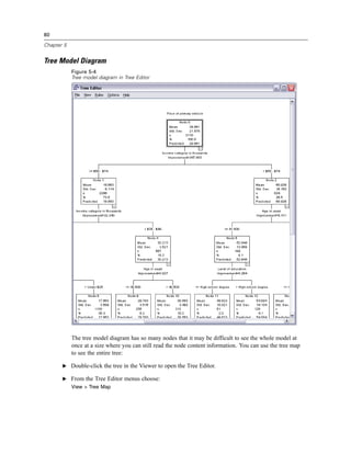
Figure 4-9
Tree table for credit rating
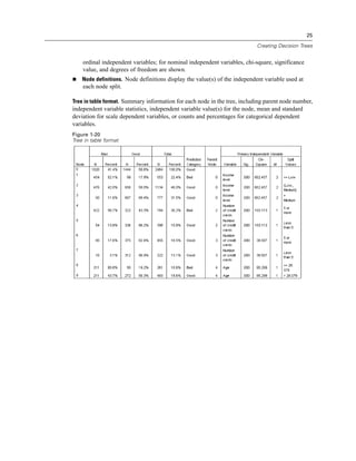
The tree table, as the name suggests, provides most of the essential tree diagram information in the
form of a table. For each node, the table displays:
 The number and percentage of cases in each category of the dependent variable.
 The predicted category for the dependent variable. In this example, the predicted category
is the credit rating category with more than 50% of cases in that node, since there are only
two possible credit ratings.
 The parent node for each node in the tree. Note that node 1—the low income level node—is
not the parent node of any node. Since it is a terminal node, it has no child nodes.
Figure 4-10
Tree table for credit rating (continued)
 The independent variable used to split the node.
 The chi-square value (since the tree was generated with the CHAID method), degrees of
freedom (df), and significance level (Sig.) for the split. For most practical purposes, you
will probably be interested only in the significance level, which is less than 0.0001 for all
splits in this model.
 The value(s) of the independent variable for that node.
Note: For ordinal and scale independent variables, you may see ranges in the tree and tree table
expressed in the general form (value1, value2], which basically means “greater than value1 and
less than or equal to value2.” In this example, income level has only three possible values—Low,

65
Medium, and High—and (Low, Medium] simply means Medium. In a similar fashion, >Medium
means High.
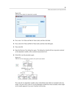
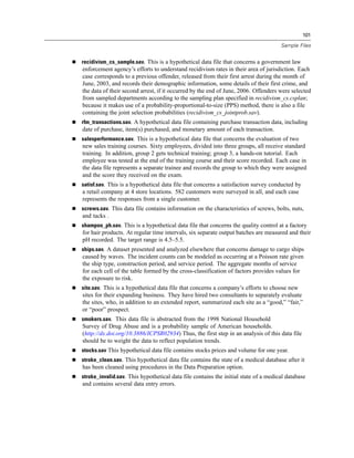
Gains for Nodes
Figure 4-11
Gains for nodes
The gains for nodes table provides a summary of information about the terminal nodes in the
model.
 Only the terminal nodes—nodes at which the tree stops growing—are listed in this table.
Frequently, you will be interested only in the terminal nodes, since they represent the best
classification predictions for the model.
 Since gain values provide information about target categories, this table is available only if
you specified one or more target categories. In this example, there is only one target category,
so there is only one gains for nodes table.
 Node N is the number of cases in each terminal node, and Node Percent is the percentage
of the total number of cases in each node.
 Gain N is the number of cases in each terminal node in the target category, and Gain Percent is
the percentage of cases in the target category with respect to the overall number of cases in the
target category—in this example, the number and percentage of cases with a bad credit rating.
 For categorical dependent variables, Response is the percentage of cases in the node in the
specified target category. In this example, these are the same percentages displayed for the
Bad category in the tree diagram.
 For categorical dependent variables, Index is the ratio of the response percentage for the target
category compared to the response percentage for the entire sample.
Index Values
The index value is basically an indication of how far the observed target category percentage
for that node differs from the expected percentage for the target category. The target category
percentage in the root node represents the expected percentage before the effects of any of the
independent variables are considered.
An index value of greater than 100% means that there are more cases in the target category than
the overall percentage in the target category. Conversely, an index value of less than 100% means
there are fewer cases in the target category than the overall percentage.

66
Chapter 4
Gains Chart
Figure 4-12
Gains chart for bad credit rating target category
This gains chart indicates that the model is a fairly good one.
Cumulative gains charts always start at 0% and end at 100% as you go from one end to the other.
For a good model, the gains chart will rise steeply toward 100% and then level off. A model that
provides no information will follow the diagonal reference line.
Index Chart
Figure 4-13
Index chart for bad credit rating target category
The index chart also indicates that the model is a good one. Cumulative index charts tend to start
above 100% and gradually descend until they reach 100%.

67
For a good model, the index value should start well above 100%, remain on a high plateau as you
move along, and then trail off sharply toward 100%. For a model that provides no information, the
line will hover around 100% for the entire chart.
Risk Estimate and Classification
Figure 4-14
Risk and classification tables
The risk and classification tables provide a quick evaluation of how well the model works.
 The risk estimate of 0.205 indicates that the category predicted by the model (good or bad
credit rating) is wrong for 20.5% of the cases. So the “risk” of misclassifying a customer is
approximately 21%.
 The results in the classification table are consistent with the risk estimate. The table shows
that the model classifies approximately 79.5% of the customers correctly.
The classification table does, however, reveal one potential problem with this model: for those
customers with a bad credit rating, it predicts a bad rating for only 65% of them, which means that
35% of customers with a bad credit rating are inaccurately classified with the “good” customers.

68
Chapter 4
Predicted Values
Figure 4-15
New variables for predicted values and probabilities
Four new variables have been created in the active dataset:
NodeID. The terminal node number for each case.
PredictedValue. The predicted value of the dependent variable for each case. Since the dependent
variable is coded 0 = Bad and 1 = Good, a predicted value of 0 means that the case is predicted
to have a bad credit rating.
PredictedProbability. The probability that the case belongs in each category of the dependent
variable. Since there are only two possible values for the dependent variable, two variables
are created:
 PredictedProbability_1. The probability that the case belongs in the bad credit rating category.
 PredictedProbability_2. The probability that the case belongs in the good credit rating category.
The predicted probability is simply the proportion of cases in each category of the dependent
variable for the terminal node that contains each case. For example, in node 1, 82% of the cases
are in the bad category and 18% are in the good category, resulting in predicted probabilities of
0.82 and 0.18, respectively.
For a categorical dependent variable, the predicted value is the category with the highest
proportion of cases in the terminal node for each case. For example, for the first case, the predicted
value is 1 (good credit rating), since approximately 56% of the cases in its terminal node have a
good credit rating. Conversely, for the second case, the predicted value is 0 (bad credit rating),
since approximately 81% of cases in its terminal node have a bad credit rating.
If you have defined costs, however, the relationship between predicted category and predicted
probabilities may not be quite so straightforward. For more information, see the topic Assigning
Costs to Outcomes on p. 72.

69
Refining the Model
Overall, the model has a correct classification rate of just under 80%. This is reflected in most
of the terminal nodes, where the predicted category—the highlighted category in the node—is
the same as the actual category for 80% or more of the cases.
There is, however, one terminal node where cases are fairly evenly split between good and
bad credit ratings. In node 9, the predicted credit rating is “good,” but only 56% of the cases in
that node actually have a good credit rating. That means that almost half of the cases in that node
(44%) will have the wrong predicted category. And if the primary concern is identifying bad
credit risks, this node doesn’t perform very well.
Selecting Cases in Nodes
Let’s look at the cases in node 9 to see if the data reveal any useful additional information.
E Double-click the tree in the Viewer to open the Tree Editor.
E Click node 9 to select it. (If you want to select multiple nodes, use Ctrl-click).
Rules > Filter Cases...
Figure 4-16
Filter Cases dialog box
The Filter Cases dialog box will create a filter variable and apply a filter setting based on the
values of that variable. The default filter variable name is filter_$.
 Cases from the selected nodes will receive a value of 1 for the filter variable.
 All other cases will receive a value of 0 and will be excluded from subsequent analyses
until you change the filter status.
In this example, that means cases that aren’t in node 9 will be filtered out (but not deleted) for now.
E Click OK to create the filter variable and apply the filter condition.

70
Chapter 4
Figure 4-17
Filtered cases in Data Editor
In the Data Editor, cases that have been filtered out are indicated with a diagonal slash through
the row number. Cases that are not in node 9 are filtered out. Cases in node 9 are not filtered;
so subsequent analyses will include only cases from node 9.
Examining the Selected Cases
As a first step in examining the cases in node 9, you might want to look at the variables not used
in the model. In this example, all variables in the data file were included in the analysis, but two
of them were not included in the final model: education and car loans. Since there’s probably a
good reason why the procedure omitted them from the final model, they probably won’t tell us
much, but let’s take a look anyway.
Analyze > Descriptive Statistics > Crosstabs...

71
Figure 4-18
Crosstabs dialog box
E Select Credit rating for the row variable.
E Select Education and Car loans for the column variables.
E Click Cells.
Figure 4-19
Crosstabs Cell Display dialog box
E In the Percentages group, select (check) Row.
E Then click Continue, and in the main Crosstabs dialog box, click OK to run the procedure.

72
Chapter 4
Examining the crosstabulations, you can see that for the two variables not included in the model,
there isn’t a great deal of difference between cases in the good and bad credit rating categories.
Figure 4-20
Crosstabulations for cases in selected node
 For education, slightly more than half of the cases with a bad credit rating have only a high
school education, while slightly more than half with a good credit rating have a college
education—but this difference is not statistically significant.
 For car loans, the percentage of good credit cases with only one or no car loans is higher than
the corresponding percentage for bad credit cases, but the vast majority of cases in both
groups has two or more car loans.
So, although you now get some idea of why these variables were not included in the final model,
you unfortunately haven’t gained any insight into how to get better prediction for node 9. If
there were other variables not specified for the analysis, you might want to examine some
of them before proceeding.
Assigning Costs to Outcomes
As noted earlier, aside from the fact that almost half of the cases in node 9 fall in each credit
rating category, the fact that the predicted category is “good” is problematic if your main
objective is to build a model that correctly identifies bad credit risks. Although you may not be
able to improve the performance of node 9, you can still refine the model to improve the rate of
correct classification for bad credit rating cases—although this will also result in a higher rate of
misclassification for good credit rating cases.
First, you need to turn off case filtering so that all cases will be used in the analysis again.
Data > Select Cases...

73
E In the Select Cases dialog box, select All cases, and then click OK.
Figure 4-21
Select Cases dialog box
E Open the Decision Tree dialog box again, and click Options.

74
Chapter 4
E Click the Misclassification Costs tab.
Figure 4-22
Options dialog box, Misclassification Costs tab
E Select Custom, and for Bad Actual Category / Good Predicted Category, enter a value of 2.
This tells the procedure that the “cost” of incorrectly classifying a bad credit risk as good is twice
as high as the “cost” of incorrectly classifying a good credit risk as bad.
E Click Continue, and then in the main dialog box, click OK to run the procedure.

75
Figure 4-23
Tree model with adjusted cost values
At first glance, the tree generated by the procedure looks essentially the same as the original tree.
Closer inspection, however, reveals that although the distribution of cases in each node hasn’t
changed, some predicted categories have changed.
For the terminal nodes, the predicted category remains the same in all nodes except one:
node 9. The predicted category is now Bad even though slightly more than half of the cases
are in the Good category.
Since we told the procedure that there was a higher cost for misclassifying bad credit risks as
good, any node where the cases are fairly evenly distributed between the two categories now has a
predicted category of Bad even if a slight majority of cases is in the Good category.

76
Chapter 4
This change in predicted category is reflected in the classification table.
Figure 4-24
Risk and classification tables based on adjusted costs
 Almost 86% of the bad credit risks are now correctly classified, compared to only 65% before.
 On the other hand, correct classification of good credit risks has decreased from 90% to 71%,
and overall correct classification has decreased from 79.5% to 77.1%.
Note also that the risk estimate and the overall correct classification rate are no longer consistent
with each other. You would expect a risk estimate of 0.229 if the overall correct classification rate
is 77.1%. Increasing the cost of misclassification for bad credit cases has, in this example, inflated
the risk value, making its interpretation less straightforward.
Summary
You can use tree models to classify cases into groups identified by certain characteristics, such as
the characteristics associated with bank customers with good and bad credit records. If a particular
predicted outcome is more important than other possible outcomes, you can refine the model to
associate a higher misclassification cost for that outcome—but reducing misclassification rates for
one outcome will increase misclassification rates for other outcomes.

Chapter
5
Building a Scoring Model
One of the most powerful and useful features of the Decision Tree procedure is the ability to build
models that can then be applied to other data files to predict outcomes. For example, based on a
data file that contains both demographic information and information on vehicle purchase price,
we can build a model that can be used to predict how much people with similar demographic
characteristics are likely to spend on a new car—and then apply that model to other data files
where demographic information is available but information on previous vehicle purchasing is not.
For this example, we’ll use the data file tree_car.sav. For more information, see the topic
Sample Files in Appendix A in IBM SPSS Decision Trees 20.
Building the Model
Figure 5-1
E Select Price of primary vehicle as the dependent variable.
E Select all the remaining variables as independent variables. (The procedure will automatically
exclude any variables that don’t make a significant contribution to the final model.)

78
Chapter 5
E For the growing method, select CRT.
E Click Output.
Figure 5-2
Output dialog box, Rules tab
E Click the Rules tab.
E Select (check) Generate classification rules.
E For Syntax, select IBM® SPSS® Statistics.
E For Type, select Assign values to cases.
E Select (check) Export rules to a file and enter a filename and directory location.
Remember the filename and location or write it down because you’ll need it a little later. If you
don’t include a directory path, you may not know where the file has been saved. You can use the
Browse button to navigate to a specific (and valid) directory location.
E Click Continue, and then click OK to run the procedure and build the tree model.
Evaluating the Model
Before applying the model to other data files, you probably want to make sure that the model
works reasonably well with the original data used to build it.

79
Building a Scoring Model
Model Summary
Figure 5-3
Model summary table
The model summary table indicates that only three of the selected independent variables made a
significant enough contribution to be included in the final model: income, age, and education.
This is important information to know if you want to apply this model to other data files, since
the independent variables used in the model must be present in any data file to which you want
to apply the model.
The summary table also indicates that the tree model itself is probably not a particularly simple
one since it has 29 nodes and 15 terminal nodes. This may not be an issue if you want a reliable
model that can be applied in a practical fashion rather than a simple model that is easy to describe
or explain. Of course, for practical purposes, you probably also want a model that doesn’t rely on
too many independent (predictor) variables. In this case, that’s not a problem since only three
independent variables are included in the final model.

Ibm spss decision_trees

Recommended

Recommended

More Related Content

What's hot

What's hot (13)

Similar to Ibm spss decision_trees

Similar to Ibm spss decision_trees (20)

Recently uploaded

Recently uploaded (20)

Ibm spss decision_trees