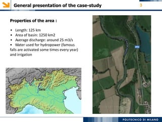
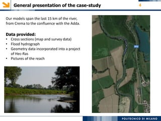
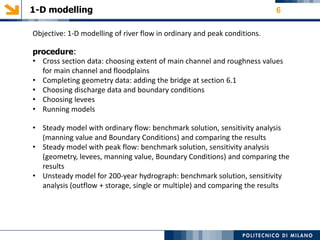
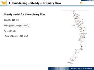
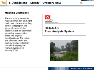
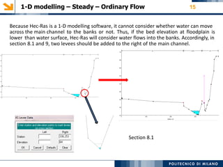
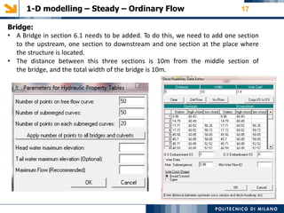
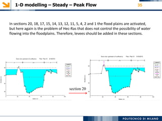
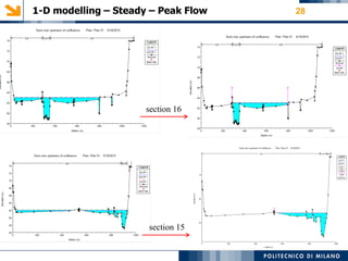
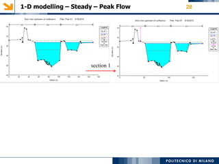
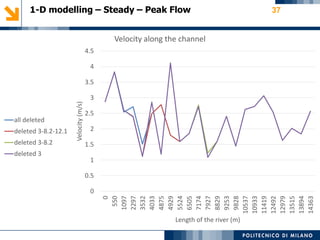
Flood Hydraulics project
Prof. Alessio Radice
Ing. Gianluca Crotti
Group Members
Majid Mohseni
Daniel Jalili
Roham Akbarian
Somi Vivek
General presentation of the case-study 2
Introduction to the
Area
The serio river is a river
located entirely within
the region Lombardy in
the north of Italy. This
river is also crossing the
provinces of Bergamo and
Cremona and flows into
the Adda River at Bocca di
Serio to the south of
Crema.
General presentation of the case-study 3
Properties of the area :
• Length: 125 km
• Area of basin: 1250 km2
• Average discharge: around 25 m3/s
• Water used for hydropower (famous
falls are activated some times every year)
and irrigation
General presentation of the case-study 4
Our models span the last 15 km of the river,
from Crema to the confluence with the Adda.
Data provided:
• Cross sections (map and survey data)
• Flood hydrograph
• Geometry data incorporated into a project
of Hec‐Ras
• Pictures of the reach
General presentation of the case-study 5
1-D modelling 6
Objective: 1‐D modelling of river flow in ordinary and peak conditions.
procedure:
• Cross section data: choosing extent of main channel and roughness values
for main channel and floodplains
• Completing geometry data: adding the bridge at section 6.1
• Choosing discharge data and boundary conditions
• Choosing levees
• Running models
• Steady model with ordinary flow: benchmark solution, sensitivity analysis
(manning value and Boundary Conditions) and comparing the results
• Steady model with peak flow: benchmark solution, sensitivity analysis
(geometry, levees, manning value, Boundary Conditions) and comparing the
results
• Unsteady model for 200-year hydrograph: benchmark solution, sensitivity
analysis (outflow + storage, single or multiple) and comparing the results
1-D modelling 7
Theoretical Background
HEC-RAS as an 1-D modelling software is based on the Saint Venant Equations.
These equations are obtained based on the following assumptions, generally
satisfied in hydraulic processes:
• All the quantities can be described as continuous and derivable functions
longitudinal position (s) and time (t).
• Fluid is uncompressible.
• flow is one-dimensional.
• Flow is fully turbulent.
• Flow is gradually varied, and the pressure is distributed hydrostatically.
Bed slope is small enough to consider cross sections as vertical. Channel
is prismatic in shape.
Continuity equation
Momentum equation
1-D modelling 8
For special cases, these equations can be simplified as follows:
Steady flow with no temporal variation:
Steady flow with no spatial and temporal variability (Uniform flow):
In case of steady flow, modelling is simple: a constant discharge should be assign to
the entire reach, and a boundary condition for water level which would be at
upstream for supercritical flows or at downstream for subcritical flows.
1-D modelling 9
In case of unsteady flow, an initial condition is necessary together with an
upstream boundary condition (usually a discharge hydrograph) and a second
boundary condition which must be upstream for supercritical flows or downstream for
subcritical flow.
Characteristic depths
Critical Depth dc:
The depth for which the specific energy is
minimum is called the critical depth.
When d>dc the flow is called supercritical
(velocity larger than that for critical flow).
When d<dc the flow is subcritical.
1-D modelling 10
Normal Depth d0:
If no quantity varies with the longitudinal direction, the flow is called uniform, and
the momentum equation representing the process is 𝑆0 = 𝑆𝑓 .The depth for
which this happens is called the normal depth.
For a given discharge, Sf is a decreasing function of water depth, therefore:
d 
d 
d0 
d0 
S0  S f
S0  Sf
1-D modelling – Steady – Ordinary Flow 11
Steady model for the ordinary flow
Length: 125 km
Average discharge: 25 𝑚3/𝑠
𝑆0 = 0.15%
Area of basin: 1250 km2
1-D modelling – Steady – Ordinary Flow 12
Manning Coefficient:
The manning values for
main channel, left and right
banks are chosen according
to the topography and
given pictures of the
sections.it can be estimated
according to vegetation
areas and physical
considerations The values
are obtained from the
table which is available in
the HEC-RAS program
manual. (Version 4.1
January 2010)
1-D modelling – Steady – Ordinary Flow 13
Table of Manning
Coefficients:
1 0.035 0.035 0.035
2 0.03 0.035 0.03
2.1 0.03 0.035 0.035
3 0.03 0.026 0.032
4 0.032 0.035 0.03
5 0.03 0.03 0.035
6 0.03 0.035 0.035
6.05 0.03 0.035 0.03
6.1
6.15 0.03 0.035 0.03
7 0.03 0.034 0.03
8 0.03 0.036 0.03
8.1 0.035 0.035 0.025
8.2 0.03 0.035 0.03
9 0.031 0.035 0.031
10 0.031 0.035 0.031
11 0.031 0.035 0.031
12 0.03 0.035 0.03
12.1 0.03 0.035 0.03
13 0.035 0.03 0.035
14 0.035 0.036 0.03
15 0.035 0.035 0.035
15.1 0.035 0.035 0.035
16 0.035 0.033 0.035
17 0.03 0.035 0.03
18 0.035 0.035 0.035
19 0.03 0.03 0.03
20 0.03 0.036 0.03
STATION
left bank
mannings
main
mannings
right bank
mannings
1-D modelling – Steady – Ordinary Flow 14
Table of
Manning
Coefficients
reasons:
1 scattered brush,heavy weeds clean and straight cleared land
2 cleared land with tree stumps shallow with some stones cleared land
2.1 cleared land shallow with some stones scattered brush,heavy weeds
3 cleared land and no sprouts almost straight,no rifts,clean cleared land
4 mature row crops winding,clean and shallow high grass
5 cleared land and no sprouts straight,clean,stones light brush and trees
6 cleared land with tree stumps turning,shallow scattered brush,heavy weeds
6.05 cleared land with tree stumps turning,shallow cleared land with tree stumps
6.1 bridge bridge bridge
6.15 cleared land with tree stumps turning,shallow cleared land with tree stumps
7 cleared land shallow,stagnant and clean mature field crops
8 cleared land reach is shallow and with weeds mature field crops
8.1 scattered brush,short grass more stones ,weeds and shallow mature row crops
8.2 cleared land shallow,clean cleared land
9 cleared land shallow,weeds,stones high grass
10 cleared land clean and shallow cleared land and no sprouts
11 mature row crops clean and shallow mature field crops
12 cleared land turning ,ineffective slope mature field crops
12.1 cleared land clean and shallow cleared land
13 scattered brush,heavy weeds shallow,with some stones light brush and trees in winter
14 scattered brush,heavy weeds small winding,shallow,stagnant cleared land
15 scattered brush,heavy weeds turning,shallow, ineffective slope scattered brush,heavy weeds
15.1 scattered brush,heavy weeds turning,shallow, ineffective slope scattered brush,heavy weeds
16 scattered brush,heavy weeds turning,shallow ,stagnant scattered brush,heavy weeds
17 small grass ineffective slope,shallow cleared land
18 scattered brush,heavy weeds shallow with some stones scattered brush,heavy weeds
19 cleared land clean ,straight,shallow cleared land and no sprouts
20 high grass more weeds,turning, stones high grass
reason right bankreason mainreason left bankSTATION
1-D modelling – Steady – Ordinary Flow 15
Because Hec-Ras is a 1-D modelling software, it cannot consider whether water can move
across the main channel to the banks or not. Thus, if the bed elevation at floodplain is
lower than water surface, Hec-Ras will consider water flows into the banks. Accordingly, in
section 8.1 and 9, two levees should be added to the right of the main channel.
Section 8.1
1-D modelling – Steady – Ordinary Flow 16
Section 9
1-D modelling – Steady – Ordinary Flow 17
Bridge:
• A Bridge in section 6.1 needs to be added. To do this, we need to add one section
to the upstream, one section to downstream and one section at the place where
the structure is located.
• The distance between this three sections is 10m from the middle section of
the bridge, and the total width of the bridge is 10m.
1-D modelling – Steady – Ordinary Flow 18
Bridge:
1-D modelling – Steady – Ordinary Flow 19
Discharge and boundary conditions:
In the case of steady flow we have to input an initial value of discharge, constant in all
along the river. To make this we have used 2 different values for discharge:
Ordinary flow 𝑄 = 25 𝑚3
/𝑠;
Peak flow Q= 561.12 𝑚3
/s;
The boundary conditions for the river depend on the nature of the flow. In the case of
subcritical flow, we have to input just downstream condition and for supercritical flows,
just upstream condition is needed.
1-D modelling – Steady – Ordinary Flow 20
Sensitivity Analysis for the Ordinary Flow
In this case we have to do sensitivity analysis of boundary conditions and the manning
values for the main channel, left and right bank to compare the influence on the water
surface elevation and velocity.
We started with both upstream and downstream conditions, for the first case we define
critical depth and for the next one we put normal depth, by defining the slope of our
main channel equal to 0.15%. Because the Froud Number along the channel is lower
than 1, Therefore, the flow is subcritical and just downstream boundary condition has to
be set and the choice of upstream boundary condition will not affect the final result.
1-D modelling – Steady – Ordinary Flow 21
1- Sensitivity Analysis of Boundary Conditions for the Ordinary Flow
To check the sensitivity of the results with respect to the boundary conditions, 4 sets
of boundary conditions are considered and their results are compared:
• Upstream critical flow and downstream normal flow (S=0.0015)
• Downstream normal flow (S=0.0015)
• Downstream critical flow
• Downstream fixed water surface elevation: 1.6m depth
1-D modelling – Steady – Ordinary Flow 22
45
47
49
51
53
55
57
59
61
63
0
550
1097
1501
2297
3532
4033
4875
4880
4890
4895
5490
6471
7140
7546
7893
8795
9219
9794
10095
10503
10899
11385
11777
12458
12945
13481
13860
14329
Elevation(m)
Length of the river (m)
Water elevation for different B.Cs
critical flow (upstream) normal
flow ( downstream)
normal flow (downstream)
critical flow (downstream)
Downstream fixed water surface
elevation: 1.6 m depth
1-D modelling – Steady – Ordinary Flow 23
0
0.5
1
1.5
2
2.5
0
550
1097
1501
2297
3532
4033
4875
4929
5524
6505
7174
7580
7927
8829
9253
9828
10129
10537
10933
11419
11811
12492
12979
13515
13894
14363
Velocity(m/s)
Length of the river (m)
Velocity along the channel for different B.Cs
critical flow (upstream) normal
flow ( downstream)
normal flow (downstream)
critical flow (downstream)
Downstream fixed water surface
elevation: 47.3 m depth
1-D modelling – Steady – Ordinary Flow 24
By comparing the result it is obvious that changing boundary conditions in the case of
ordinary flow, does not influence water surface elevation and velocity along the river
except few last sections due to different downstream boundary conditions.
Serio river profile in HEC-RAS
Longitudinal Profile
1-D modelling – Steady – Ordinary Flow 25
2-Roughness Sensitivity Analysis
In order to perform the sensitivity analysis of the roughness of the river the manning
values are increased once for +0.01 and another time reduced for -0.01 and we have
compared these two different cases in manning values with the original one to
understand the differences on the water surface elevation and velocity.
2-1-Roughness sensitivity analysis on water surface elevation
It can be observed, the increasing of the Manning values has an effect of the increasing in
the water surface elevation and vice versa, which means the graph plotted the Manning
value +0.01 is higher than the others. However, the change in water surface elevation is
insignificant.
1-D modelling – Steady – Ordinary Flow 26
45
47
49
51
53
55
57
59
61
63 0
550
1097
1501
2297
3532
4033
4875
4880
4890
4895
5490
6471
7140
7546
7893
8795
9219
9794
10095
10503
10899
11385
11777
12458
12945
13481
13860
14329
Watersurfaceelevation(m)
Length of the river (m)
Main Manning value - 0.01
Main Manning value + 0.01
Main Manning value
1-D modelling – Steady – Ordinary Flow 27
In the distance of 10-11 Km, where the bridge is located, water surface of the different
Manning values are meeting at the same elevation, in this section, the reason of this
occurrence might be because of contraction of the bridge piers and there is a critical
condition. From Froud numbers that calculated in HEC-RAS we have subcritical flow
before and supercritical flow after the bridge, as a result the flow in the bridge section
is critical.
1-D modelling – Steady – Ordinary Flow
2-2-Roughness sensitivity analysis on velocity along the river
According to graph it is obvious that the effect of modification of the Manning values
is remarkable on velocity magnitude, which means if the roughness increases the
magnitude of velocity will decrease and vice versa,
0
0.5
1
1.5
2
2.5
0
550
1097
1501
2297
3532
4033
4875
4929
5524
6505
7174
7580
7927
8829
9253
9828
10129
10537
10933
11419
11811
12492
12979
13515
13894
14363
Velocity(m/s)
Length of the river (m)
Main Manning value -0.01
Main Manning value +0.01
Main Manning value
28
1-D modelling – Steady – Peak Flow 29
Steady model for the peak flow
Length: 125 km
Average discharge: 560 m3/s
S0= 0.15%
The geometry of the model is the same as the ordinary
flow, except for 4 sections that are deleted and 15
sections in which levees are added.
1-D modelling – Steady – Peak Flow 30
Sections 15.1, 12.1, 8.2 and 3 are deleted.
1-D modelling – Steady – Peak Flow 30
In the case of sections 15.1, 8.2 and the general direction of the flood would be
vertically down. Since the sections are too narrow and located after a bend in the main
river, all the sections will be flooded, so we can delete them.
1-D modelling – Steady – Peak Flow 30
1-D modelling – Steady – Peak Flow 31
In the case of section 12.1 since the section is too narrow it will be flooded, so it
can be deleted and also for the section 3 because it is located after a bend in the main
river, it should be deleted.
1-D modelling – Steady – Peak Flow 31
1-D modelling – Steady – Peak Flow 35
section 20
In sections 20, 18, 17, 15, 14, 13, 12, 11, 5, 4, 2 and 1 the flood plains are activated,
but here again is the problem of Hec-Ras that does not control the possibility of water
flowing into the floodplains. Therefore, levees should be added in these sections.
1-D modelling – Steady – Peak Flow 35
In the left hand side of section 16, a levee should be added to prevent unreasonable
activation of the floodplain. In the right side, since its upper section (section 17) is
narrow, all the width of the section would not be flooded but just a portion of it.
Therefore, a levee is added to the right side to take into account this issue.
Sections 6.05 and 6.15 are the same. These are sections before and after the bridge.
Since around the columns of the bridge water does not flow, 2 levees are added
parallel to the columns to consider this issue.
1-D modelling – Steady – Peak Flow 28
section 18
section 17
1-D modelling – Steady – Peak Flow 28
section 16
section 15
1-D modelling – Steady – Peak Flow 28
section 14
section 13
1-D modelling – Steady – Peak Flow 28
section 12
section 11
1-D modelling – Steady – Peak Flow 28
section 6.5
section 5
1-D modelling – Steady – Peak Flow 28
section 4
section 2
1-D modelling – Steady – Peak Flow 28
section 1
1-D modelling – Steady – Peak Flow 31
Running the model:
The longitudinal profile
1-D modelling – Steady – Peak Flow
32
Sensitivity Analysis of Boundary Conditions for the Peak Flow
To check the sensitivity of the results with respect to the boundary conditions, 4
sets of boundary conditions are considered and their results are compared:
• Upstream critical flow and downstream normal flow
• Downstream critical flow
• Downstream normal flow
• Downstream fixed water surface elevation: 5.5 m depth
45
50
55
60
65
70
0
550
1097
2297
3532
4033
4875
4880
4890
4895
5490
6471
7140
7893
8795
9219
9794
10503
10899
11385
12458
12945
13481
13860
14329
Elevation(m)
Length of the river (m)
Water elevation for different B.Cs.
critical flow (upstream) normal flow (
downstream)
normal flow (downstream)
critical flow (downstream)
Downstream fixed water surface
elevation: 5.5 m depth
1-D modelling – Steady – Peak Flow 33
It is clear that having different boundary conditions for the peak flow case does
not affect the results, except for a few sections close to the downstream which is
due to different criteria we have chosen there.
0
0.5
1
1.5
2
2.5
3
3.5
4
0
550
1097
2297
3532
4033
4875
4929
5524
6505
7174
7927
8829
9253
9828
10537
10933
11419
12492
12979
13515
13894
14363
Velocity(m/s)
Length of the river (m)
Velocity along the channel for different B.Cs
critical flow (upstream) normal flow (
downstream)
normal flow (downstream)
critical flow (downstream)
Downstream fixed water surface
elevation: 5.5 m depth
1-D modelling – Steady – Peak Flow 34
Sensitivity Analysis of the geometry for the Peak Flow
In the case of the 4 deleted sections, the water surface elevation and velocity at the
sections upper to the deleted sections and along the river reach are compared.
Since the flow is subcritical, and subcritical flows need downstream boundary
conditions, the effect of changing the geometry would be on the upper sections.
In order to check the sensitivity of the results with respect to the geometry of
the model, 2 issues are considered:
• Sensitivity of results with respect to the deleted sections
• Sensitivity of results with respect to the added levees
1-D modelling – Steady – Peak Flow 35
45
50
55
60
65
70
Elevation(m)
Length of the river (m)
Water surface along the river
all deleted deleted 3-8.2-12.1 deleted 3-8.2 deleted 3
1-D modelling – Steady – Peak Flow 37
0
0.5
1
1.5
2
2.5
3
3.5
4
4.5
0
550
1097
2297
3532
4033
4875
4929
5524
6505
7174
7927
8829
9253
9828
10537
10933
11419
12492
12979
13515
13894
14363
Velocity(m/s)
Length of the river (m)
Velocity along the channel
all deleted
deleted 3-8.2-12.1
deleted 3-8.2
deleted 3
1-D modelling – Steady – Peak Flow 38
Generally, the reference model has 15 levees at sections 5, 6.05 and 6.15(before and
after the bridge), 16, 17 and 18. In the case of the added levees, water surface
elevation and velocity along the river reach are compared for different sets of levees:
• No levee
• 1 levee at section 5 (downstream)
• 3 levees at sections 5 (downstream), 17 and 18 (upstream)
• All the 6 levees
1-D modelling – Steady – Peak Flow 39
45
50
55
60
65
70
0
550
1097
2297
3532
4033
4875
4880
4890
4895
5490
6471
7140
7893
8795
9219
9794
10503
10899
11385
12458
12945
13481
13860
14329
Elevation(m)
Length of the river (m)
Water elevation along the river with and without levees
all levees
no levee
Bed Elevation
1-D modelling – Steady – Peak Flow 40
0
0.5
1
1.5
2
2.5
3
3.5
4
4.5
0
550
1097
2297
3532
4033
4875
4929
5524
6505
7174
7927
8829
9253
9828
10537
10933
11419
12492
12979
13515
13894
14363
Velocity(m/s)
Length of the rievr (m)
Velocity along the river with and without levee
all levees
no levee
1-D modelling – Steady – Peak Flow 41
Results:
• The changes in water surface elevation along the channel due to omission of
several sections are smaller than 1%.
• The changes in water surface elevation and velocity at the upper sections of
deleted sections vary from small values up to the 60% increase in velocity at section
13.
• The changes in velocity along the channel due to omission of several sections
are mainly smaller than 20% except for the portion between deleted sections
15.1 and 12.1 in which the velocity change up to 60%.
• As a conclusion, deleting sections has a negligible effect on water surface
elevation, but the effect on velocity is noteworthy.
• The changes in water surface elevation along the channel due to adding levees
are smaller than 0.6%.
• The changes in velocity along the channel due to adding levees are mainly
smaller than 15% (specifically for the case of having all the 6 levees), for the case of
having 3 levees, the velocity changes up to 25%.
• As a conclusion, adding levees has a negligible effect on water surface elevation, but
• the effect on velocity is more and mostly in the upstream part of the
river.
1-D modelling – Steady – Peak Flow 42
70
Peak flow
65 original condition
-0.00560
-0.01
55
-0.02
50
0.005
45 0.1
0.0240
0 2000 4000 6000 8000 10000 12000 14000 16000
Distance from upstream (m)
WaterSurfaceelevation(m)
Roughness sensitivity analysis on water surface elevation
In the same manner as the previous case, the lower the manning coefficient is, the
lower is the water surface elevation and vice versa. A clear difference between this
plot with the one corresponding to the ordinary flow is that seemingly, the peak flow
condition is more sensitive to manning variation when compared to the ordinary flow.
This will be studied more in the upcoming slides. Comparing this plot with the
previous one also shows that although; in case of the ordinary flow all conditions pass
the bridge with the same water depth, in case of the peak flow, this phenomena is
not observed.
1-D modelling – Steady – Peak Flow 43
1.50
Station 10
1.00
0.50
0.00
-80.0 -60.0 -40.0 -20.0 0.0 20.0 40.0 60.0 80.0
-0.50
-1.00
ordinary flow
Peak flow
-1.50
-2.00
Manning coefficient variation (% refrence value)
WaterSurfacevariation(%refrencevaalue)To study better the sensitivity, the values are compared based on the percentage of
variation in comparison to the control model. To study the phenomena from this
perspective, the change in values of both manning coefficient and water surface
elevations are given in percentage. The figure below represents the results
obtained for a general section along the river channel (section 10). In this plot, the
percentage of water surface variation is plotted against the percentage of manning
coefficient variation.
1-D modelling – Steady – Peak Flow 44
1.50
1.00
0.50
0.00
-80.0 -60.0 -40.0 -20.0 0.0 20.0 40.0 60.0 80.0
-0.50
-1.00
ordinary flow
Peak flow
-1.50
-2.00
Manning coefficient variation (% refrence value)
WaterSurfacevariation(%refrencevaalue)
For this specific location, it is seen that the variation of the manning coefficient has a
more pronounced effect on the peak flow discharge compared to the discharge with
ordinary flow. Another conclusion that may be drawn from the figure is that,
decreasing the manning value has affected the water surface elevation more notably
especially for the peak flow discharge. Although the manning variation shows to
influence the water surface elevation, this effect is less than 2 percent even in the
point with highest influence, so generally speaking, the effect of manning coefficient
is negligible.
1-D modelling – Steady – Peak Flow 45
1.00
0.80
0.60
0.40
highest water depth
0.00
-80.0 -60.0 -40.0 -20.0
-0.20 0.0 20.0 40.0 60.0 80.0
low water depth
-0.40
-0.60
-0.80
-1.00
Manning coefficient variation (% refrence value)
WaterSurfacevariation(%refrencevaalue)
0.20
Here is also presented the plot of water surface elevation change versus
manning coefficient changes for the point with highest water depth and for a
point with a low water depth for the ordinary flow condition, to study
whether the sensitivity may change with water depth. Based on the figure,
the water depth does not seem to be an influential factor on roughness
sensitivity as the trends visible for both curves seem to be similar.
1-D modelling – Steady – Peak Flow 46
Roughness sensitivity analysis on velocity along the river
6
5
original
-0.005
-0.01
-0.02
0.005
0.01
0.02
4
3
2
1
0
0 2000 4000 6000 8000 10000 12000 14000 16000
Distance from upstream (m)
velocity(m/s)
Here is plotted the velocity against manning coefficient changes for the peak
flow. The same behavior is observed as for the ordinary flow.
1-D modelling – Steady – Peak Flow 47
2.50
2.00
-0.02
-0.01
-0.005
0.005
0.01
0.02
1.50
1.00
0.50
0.00
0 2000 4000 6000 8000 10000 12000 14000 16000
distance from upstream (m)
normalizedvelocity
Again the same trend is observed as of the ordinary flow, except that the
increase in velocity for the reduction of 0.02 in manning coefficient is more
pronounced to comparison with the ordinary flow. For the other values, the
results almost resemble the ones for ordinary flow.
1-D modelling – Unsteady – Peak Flow 48
Unsteady model for 200-year Hydrograph
In unsteady modeling, all the parameters from previous models are used, except for
the levees.
1. Model conditions
Boundary condition
• Upstream: 200-year hydrograph
• Downstream: normal depth with slope of 0.0015
Initial condition
• Initial discharge
• Storage water surfaces ( if applicable )
2. Trial running and detecting possible storage areas
All the levees are removed because we are going to simulate the floodplain using
storage areas. The first step is to find possible floodplain(s) according to section
geometry, map and water level.
3. Running the model
Detected storage areas are used to run several different models in order to check the
influences of storage areas.
1-D modelling – Unsteady – Peak Flow 49
Unsteady flow data
The original dataset is interpolated with 30-minute time interval (using Matlab
software). This time interval is small enough with respect to the whole event history.
Upstream Hydrograph
1-D modelling – Unsteady – Peak Flow 50
Locating storage areas
To located the appropriate locations for storages different factors should be
considered:
Map: considering the overall condition of the river shore such as not having
residential areas
Water level: the possibility of water to flow from the main channel to the storage
Geometry of the sections: considering up- and downstream sections of chosen
section and the possibility of having a storage in that part of the river
A few simplification assumptions are employed for the modeling:
1. All the storage areas have plane beds;
2. The elevation of each storage area is the minimum elevation between its
up- and downstream sections.
3. The weirs connecting main channel and storage areas are 100m long and
100m wide.
4. The areas are roughly calculated by hand-drawing.
1-D modelling – Unsteady – Peak Flow 51
Locating storage areas
Some storage areas are chosen as shown in the
right figure. Most of them are located at turning
sections of the river.
52
Final layout of storage areas
elevation
Storage
Area
(1000m2)
Min.
18-17 86 63
17-16 238 62
16-15 151 61.5
15-14 175 60.5
13-12 173 59
11-10 244 59
10-9 203 58
1-D modelling – Unsteady – Peak Flow
1-D modelling – Unsteady – Peak Flow 53
Sensitivity
width
analysis regarding number of storages, interpolation length and weir
As it is shown, by increasing
(adding
the
from
the
number of storages
upstream to downstream),
and maximum
Therefore,
both
wave volume discharge
are reduced. we can
conclude that more storages can help us
control the flood in a more efficient
way.
Steps Qmax
Wave Volume
(1000m3)
Upstream 561.84 91377.24
0 storage 541.21 91276.98
1 storage 541.13 91276.29
2 storages 526.87 91002.2
3 storages 520.3 90822.13
4 storages 520.54 90810.33
5 storages 518.48 90730.41
6 storages 518.48 90730.41
7 storages 517.78 90570.32
1-D modelling – Unsteady – Peak Flow 54
Interpolation of sections
The model with 7 storages is set as the reference model to analyze interpolation effects.
Interpolation
length
Qmax Wave Volume
(1000m3)
Origin sections 517.78 90570.32
500m 516.56 90550.19
400m 516.51 90558.79
300m 516.55 90556.01
200m 516.6 90557.49
As it is shown, by increasing the number
of storages (adding from upstream to
downstream), both the wave volume and
maximum discharge are reduced.
Therefore, we can conclude that more
storages can help us control the flood in a
more efficient way.
1-D modelling – Unsteady – Peak Flow 55
Weir width effect
*The lower lines are the hydrographs
of storages.
Down stream hydrographs of 100m weir width
Down stream hydrographs of 500m weir width
Weirs are used to simulate
the connection parts
between the channel and the
storages. Two kinds of weir
widths with 100m and 500m
are set.
A wider weir is possible in
order to have a better
description of the reality, but
it may introduce
computational instability or
complex simulation results.
562-D modelling
Theoretical Background
The numerical formulation of 2D river
modelling was originated from the analysis of
shallow water. The main outputs of the 2D
model are two water velocity components and
a vertical water depth for each defined node.
Basically, the output of the program is
generated by the solution of the mass
conservation equation and the two
momentum conservation equations.
2-D modelling 57
The 2D model depth averaged, mass and momentum conservation equations are:
The bed shear stress are computed by: and
The turbulent normal and shear stresses are computed according to the
Boussinesq’s assumption as:
2-D modelling 58
Benefits:
Limitations:
• Ability to model more complex flows
including floodplain and underground
flows
• Ability to consider impact of
obstructions.
• No need to force the geometry to be
appropriate for modelling
• Results are limited by the accuracy of the
assumptions, input data and the computing
power of the computer program.
• Modeling complexity and precision are not
a substitute for sound engineering
judgment.
2-D modelling 59
Comparing the results of 2-D with 1-D modelling
Since River 2D results 2 values for velocity along the X and Y
axes, and computes the water depth at each node, it is not
possible to have single longitudinal profiles for velocity and
water surface for the river. Therefore, the results are compared
section by section.
Water Surface Elevation
The comparisons for the first and last sections are neglected due
to less accuracy of results in these sections.
Section 19
67
66
65
64
63
62
61
60
59
ws
Bed
0 20 40
Station (m)
60 80
Elevation(m)
2-D modelling (sections 18 &
1-D
17) 60
2-D
74
72
70
68
66
64
62
60
58
bed
ws
0 200 400
Station (m)
600 800
74
72
70
68
66 bed
ws64
62
60
58
0 200 400 600 800 1000
Station (m)
Elevation(m)Elevation(m)
2-D modelling (sections 18 & 17) 61
When water flows from a narrow section upstream to a wider section at downstream, the
17.width of the flow expands gradually. That is what is happening in section 19 to 18 and
The difference in the results is because of the lower results for water surface elevations in
sections 18 and 17 by Hec-Ras, and by that lower values, floodplains would not be
activated. This is the reason why we put the levees there in the first place.
2-D modelling (section 16) 62
1-D 2-D
74
72
70
68
66 Bed
WS
64
62
60
58
0 200 400 600 800 1000 1200
Station (m)
In section 16, since we considered water exists only in the main channel in its upper section
(section 17), therefore again we would have the expanding flow phenomena here, and we
were only a little wrong about the place of the levee, but if we knew that the upper section’s
floodplain is already activated, we would have put the levee further to the right, or even
remove the levee to completely activate the floodplain.
Elevation(m)
2-D modelling (section 15) 63
From section 15 on, since we were aware of activation of the floodplains, and by exploring
the topography of the river and sections, it was decided not to put any levee. Therefore, the
results are reasonably similar regarding the activation of the flood plains.
74
72
70
68
66
64
62
60
58
56
bed
ws
0 200 400 600
Station (m)
800 1000 1200
Elevation(m)
2-D modelling (sections 14 & 13) 64
1-D 2-D
75
73
71
69
67
65
63
61
59
57
55
bed
ws
0 200 400 600 800 1000 1200
75
70
Bed
WS
65
60
55
0 200 400 600 800 1000 1200
2-D modelling (sections 12 & 11) 65
1-D 2-D
72
70
68
66
64
Bed
WS
62
60
58
56
54
0 200 400 600 800 1000
75
70
65
Bed
WS60
55
50
0 200 400 600 800 1000
2-D modelling (sections 10 & 9) 66
1-D 2-D
75
70
65
Bed
WS60
55
50
0 100 200 300 400 500 600 700 800
72
70
68
66
64
Bed
WS62
60
58
56
54
0 200 400 600 800 1000 1200
2-D modelling (section 8.1) 67
1-D 2-D
70
68
66
64
Bed
WS
62
60
58
56
54
0 100 200 300 400 500
General Comments:
 As it is clear, the water surface elevations resulted from River 2D are more accurate
than Hec-Ras in which a single value is reported for each section
 Generally, River 2D has obtained higher water surface elevations along the river which
results in activation of more floodplains.
 Except for sections 18, 17 and 16, results of the two software are different but in a
reasonable way
2-D modelling - Velocity 68
Station 18Station 19
4.5
4
3.5
3
2.5
2
1.5
1
0.5
0
5
4.5
4
3.5
3
2.5
2
1.5
1
0.5
0
1D
2D
2-D
1D
0 100 200 300 400 500
0 20 40
Station (m)
60 80 Station (m)
Station 17 Station 16
4.5
4
3.5
3
2.5
2
1.5
1
0.5
0
3
2.5
2
1.5
2D
1D
1D
2D1
0.5
0
0 200 400
Station (m)
600 800 0 200 400 600 800 1000
Station (m)
Velocity(m/s)Velocity(m/s)
Velocity(m/s)Vercity(m/s)
2-D modelling - Velocity 69
Station 14Station 15
2.5
7
6
5
4
3
2
1
0
2
1.5
1D
2D
1
1D
2D
0.5
0
0 200 400 600 800 1000
0 200 400 600 800 1000
Station (m)
Station (m)
Station 12Station 13
3
1.8
1.6
1.4
1.2
1
0.8
0.6
0.4
0.2
0
2.5
2
1.5
1D
2D
1D
2D
1
0.5
0
0 200 400
Station (m)
600 800 0 200 400 600 800 1000
Station (m)
Velocity(m/s)Velocity(m/s)
Velocity(m/s)
Velocity(m/s)
2-D modelling - Velocity 70
Station 10Station 11
3
4.5
4
3.5
3
2.5
2
1.5
1
0.5
0
2.5
2
1.5
1D
2D
1D
2D1
0.5
0
0 200 400
Station (m)
600 8000 200 400 600 800 1000
Station (m)
Station 9 Station 8-1
1.4 1.6
1.41.2
1.21
10.8
0.81D
2D
1D
2D
0.6
0.6
0.4
0.4
0.2
0.2
0
00 200 400 600 800 1000
0 100 200
Station (m)
300 400
Station (m)
Velocity(m/s)Velocity(m/s)
Velocity(m/s)
Velocity(m/s)
2-D modelling - Velocity 71
General Comments:
The differences in the values of velocity obtained
by the two software are because:
 River 2D considers two components for
velocity (in X direction and Y direction), but
Hec-Ras considers only velocity for each
section along the channel (so perpendicular to
the cross sections).
 In 2D modelling, lateral stresses are also
considered while in the 1D modelling only
friction losses are considered.
Vulnerability and Risk assessment 72
RISK = f ( HAZARD, VULNERABILITY,
EXPOSURE)
RISK is measured in terms of expected damage, such as
expected number of lives lost, persons injured, damages
to properties and disruption of economic activities due to
a particular natural phenomenon (in this case flood).
 Hazard = characteristics of the dangerous phenomena
(Flood)
 Vulnerability = propensity to damage, fragility
 Exposed systems = number and dimension of people
and goods in a dangerous area
Hazard Vulnerability
Risk
Strong
W
mber
of
ople
Vulnerability and Risk assessment 73
Hazard:
To evaluate hazard in flooded area, we should consider the
water surface level at affected items and also the flood
duration:
 Our hazard input was the hydrograph that shows
discharge for almost five days .
 The severity of the hazard depends on the duration of
flooding and water elevation
 The floodplains are where the risk should be evaluate
 The return period is 200 years in our case.
When
here
How
Economics
Exposure:
Exposure can be Estimated in affected area as the number of
people, houses and economic activities involved.
Buildings
Nu
p
e
Vulnerability and Risk assessment 74
5022000.00
5021000.00
5020000.00
boundary 2D model
river axis
edge of water
towns
farm houses and stores
isolated historical-religious
major roads
5019000.00
5018000.00
5017000.00
5016000.00
5015000.00
553500.00 554500.00 555500.00 556500.00 557500.00
According to the above map which can be considered as the exposure map, there are
just several farms within the edge of water zone. Therefore, the calculated flood
damage is considered just for damages to the farms.
Vulnerability and Risk assessment 75
Vulnerability
From all different types of vulnerability (physical, systemic, organizational and
social), the physical vulnerability is considered which is related to physical
characteristics of the affected items such as people, infrastructures and environment.
Risk evaluation
According to risk components, the level of risk is evaluated in terms of expected
damage in area the expected flood.
Vulnerability and Risk assessment 76
DamageAssessment:
 Hazard: the characteristic flood with a duration less than one week
 ExposedArea = 530 ha
 Vulnerability parameters:


Type of activity
Time of year: June
Due to lack of data regarding areas dedicated to each kind of agricultural activities,
equal values are allocated to all parts.
Vulnerability and Risk assessment 77
Total Damage:
As a result, the total damage due to the considered
about 1,250,000 euro.
flood hazard in the exposed area is
Inundation less than 1 week
type of
land
dryland irrigated
dryland
corps
irrigated
corp
vegetable grapes orchard tobacco hops other SUM SUM (€)
damage/h
a
0 90 84 147 5600 2500 6000 320 486 2227 - -
A(ha) 53 53 53 53 53 53 53 53 53 53 530 € = $/0.75
damage 0 4770 4452 7791 296800 132500 318000 16960 25758 118031 $925,062 1,233,416
Final Discussion 78
The final results of our analysis stress out the necessity for measures
taken. These measure can be of two forms, non-structural and structural.
to be
Non structural measures:
• Constant monitoring
• Emergency planning
• Information technologies
• Knowledge and training
• Land-use planning
Sustainable structural measures:
Short term
• Sandbags and barriers
Long term
• Levees
• Weir and storage
Final Discussion 79
From our analysis, we concluse that the risk is high in the areas along the shores of the
Adda river.
From a non-structural point of view, a monitoring system can be set in
and check the state of the river at different times. Another important
structural measure is land-use planning. For example, in critical areas,
order to record
aspect of non-
construction of
buildings and houses can be avoided, whereas in cases of already existing structures in
critical areas, educating and emergency planning must be at the forefront.
From the structural point of view, levees, storages and weir-by-passes can be used. The
aim of this project was not only to reduce the risk in the areas surrounding the Adda
river, but also to reduce it in a sustainable way. This means optimizing the resources to
be used according to the desired results.
In case of the added storages, a significant decrease in discharge is acquired downstream
of the river, which leads to a lower level of risk and therfore damage.
Final Discussion 80
Advantage and disadvantages of different models:
Steady flow 1-D model:
 Considers only water elevation and velocity in space but not in time. To take different
velocities into account, main channels and banks have to be seperated.
Unsteady flow 1-D model:
 More realistic and accurate than steady flow model, since it represents the longitudinal
decrease of peak discharge and depth.
 The possibility to calculate wave volume and celerity.
Steady flow 2-D model
 More complex modelling than 1D model, thus more accurate results.
 Takes into account floodplains, lateral stresses, roughness, geometry, boundary
conditions, wetting and drying condition treatments.
 Velocity is calculated in two directions (x and y). Also, the inclusion of the lateral
stresses makes the velocity distibution more accurate. While 1-D models consider only
the axial direction of flow and no lateral stresses.

Hydraulics daniel

  • 1.
    Flood Hydraulics project Prof.Alessio Radice Ing. Gianluca Crotti Group Members Majid Mohseni Daniel Jalili Roham Akbarian Somi Vivek
  • 2.
    General presentation ofthe case-study 2 Introduction to the Area The serio river is a river located entirely within the region Lombardy in the north of Italy. This river is also crossing the provinces of Bergamo and Cremona and flows into the Adda River at Bocca di Serio to the south of Crema.
  • 3.
    General presentation ofthe case-study 3 Properties of the area : • Length: 125 km • Area of basin: 1250 km2 • Average discharge: around 25 m3/s • Water used for hydropower (famous falls are activated some times every year) and irrigation
  • 4.
    General presentation ofthe case-study 4 Our models span the last 15 km of the river, from Crema to the confluence with the Adda. Data provided: • Cross sections (map and survey data) • Flood hydrograph • Geometry data incorporated into a project of Hec‐Ras • Pictures of the reach
  • 5.
    General presentation ofthe case-study 5
  • 6.
    1-D modelling 6 Objective:1‐D modelling of river flow in ordinary and peak conditions. procedure: • Cross section data: choosing extent of main channel and roughness values for main channel and floodplains • Completing geometry data: adding the bridge at section 6.1 • Choosing discharge data and boundary conditions • Choosing levees • Running models • Steady model with ordinary flow: benchmark solution, sensitivity analysis (manning value and Boundary Conditions) and comparing the results • Steady model with peak flow: benchmark solution, sensitivity analysis (geometry, levees, manning value, Boundary Conditions) and comparing the results • Unsteady model for 200-year hydrograph: benchmark solution, sensitivity analysis (outflow + storage, single or multiple) and comparing the results
  • 7.
    1-D modelling 7 TheoreticalBackground HEC-RAS as an 1-D modelling software is based on the Saint Venant Equations. These equations are obtained based on the following assumptions, generally satisfied in hydraulic processes: • All the quantities can be described as continuous and derivable functions longitudinal position (s) and time (t). • Fluid is uncompressible. • flow is one-dimensional. • Flow is fully turbulent. • Flow is gradually varied, and the pressure is distributed hydrostatically. Bed slope is small enough to consider cross sections as vertical. Channel is prismatic in shape. Continuity equation Momentum equation
  • 8.
    1-D modelling 8 Forspecial cases, these equations can be simplified as follows: Steady flow with no temporal variation: Steady flow with no spatial and temporal variability (Uniform flow): In case of steady flow, modelling is simple: a constant discharge should be assign to the entire reach, and a boundary condition for water level which would be at upstream for supercritical flows or at downstream for subcritical flows.
  • 9.
    1-D modelling 9 Incase of unsteady flow, an initial condition is necessary together with an upstream boundary condition (usually a discharge hydrograph) and a second boundary condition which must be upstream for supercritical flows or downstream for subcritical flow. Characteristic depths Critical Depth dc: The depth for which the specific energy is minimum is called the critical depth. When d>dc the flow is called supercritical (velocity larger than that for critical flow). When d<dc the flow is subcritical.
  • 10.
    1-D modelling 10 NormalDepth d0: If no quantity varies with the longitudinal direction, the flow is called uniform, and the momentum equation representing the process is 𝑆0 = 𝑆𝑓 .The depth for which this happens is called the normal depth. For a given discharge, Sf is a decreasing function of water depth, therefore: d  d  d0  d0  S0  S f S0  Sf
  • 11.
    1-D modelling –Steady – Ordinary Flow 11 Steady model for the ordinary flow Length: 125 km Average discharge: 25 𝑚3/𝑠 𝑆0 = 0.15% Area of basin: 1250 km2
  • 12.
    1-D modelling –Steady – Ordinary Flow 12 Manning Coefficient: The manning values for main channel, left and right banks are chosen according to the topography and given pictures of the sections.it can be estimated according to vegetation areas and physical considerations The values are obtained from the table which is available in the HEC-RAS program manual. (Version 4.1 January 2010)
  • 13.
    1-D modelling –Steady – Ordinary Flow 13 Table of Manning Coefficients: 1 0.035 0.035 0.035 2 0.03 0.035 0.03 2.1 0.03 0.035 0.035 3 0.03 0.026 0.032 4 0.032 0.035 0.03 5 0.03 0.03 0.035 6 0.03 0.035 0.035 6.05 0.03 0.035 0.03 6.1 6.15 0.03 0.035 0.03 7 0.03 0.034 0.03 8 0.03 0.036 0.03 8.1 0.035 0.035 0.025 8.2 0.03 0.035 0.03 9 0.031 0.035 0.031 10 0.031 0.035 0.031 11 0.031 0.035 0.031 12 0.03 0.035 0.03 12.1 0.03 0.035 0.03 13 0.035 0.03 0.035 14 0.035 0.036 0.03 15 0.035 0.035 0.035 15.1 0.035 0.035 0.035 16 0.035 0.033 0.035 17 0.03 0.035 0.03 18 0.035 0.035 0.035 19 0.03 0.03 0.03 20 0.03 0.036 0.03 STATION left bank mannings main mannings right bank mannings
  • 14.
    1-D modelling –Steady – Ordinary Flow 14 Table of Manning Coefficients reasons: 1 scattered brush,heavy weeds clean and straight cleared land 2 cleared land with tree stumps shallow with some stones cleared land 2.1 cleared land shallow with some stones scattered brush,heavy weeds 3 cleared land and no sprouts almost straight,no rifts,clean cleared land 4 mature row crops winding,clean and shallow high grass 5 cleared land and no sprouts straight,clean,stones light brush and trees 6 cleared land with tree stumps turning,shallow scattered brush,heavy weeds 6.05 cleared land with tree stumps turning,shallow cleared land with tree stumps 6.1 bridge bridge bridge 6.15 cleared land with tree stumps turning,shallow cleared land with tree stumps 7 cleared land shallow,stagnant and clean mature field crops 8 cleared land reach is shallow and with weeds mature field crops 8.1 scattered brush,short grass more stones ,weeds and shallow mature row crops 8.2 cleared land shallow,clean cleared land 9 cleared land shallow,weeds,stones high grass 10 cleared land clean and shallow cleared land and no sprouts 11 mature row crops clean and shallow mature field crops 12 cleared land turning ,ineffective slope mature field crops 12.1 cleared land clean and shallow cleared land 13 scattered brush,heavy weeds shallow,with some stones light brush and trees in winter 14 scattered brush,heavy weeds small winding,shallow,stagnant cleared land 15 scattered brush,heavy weeds turning,shallow, ineffective slope scattered brush,heavy weeds 15.1 scattered brush,heavy weeds turning,shallow, ineffective slope scattered brush,heavy weeds 16 scattered brush,heavy weeds turning,shallow ,stagnant scattered brush,heavy weeds 17 small grass ineffective slope,shallow cleared land 18 scattered brush,heavy weeds shallow with some stones scattered brush,heavy weeds 19 cleared land clean ,straight,shallow cleared land and no sprouts 20 high grass more weeds,turning, stones high grass reason right bankreason mainreason left bankSTATION
  • 15.
    1-D modelling –Steady – Ordinary Flow 15 Because Hec-Ras is a 1-D modelling software, it cannot consider whether water can move across the main channel to the banks or not. Thus, if the bed elevation at floodplain is lower than water surface, Hec-Ras will consider water flows into the banks. Accordingly, in section 8.1 and 9, two levees should be added to the right of the main channel. Section 8.1
  • 16.
    1-D modelling –Steady – Ordinary Flow 16 Section 9
  • 17.
    1-D modelling –Steady – Ordinary Flow 17 Bridge: • A Bridge in section 6.1 needs to be added. To do this, we need to add one section to the upstream, one section to downstream and one section at the place where the structure is located. • The distance between this three sections is 10m from the middle section of the bridge, and the total width of the bridge is 10m.
  • 18.
    1-D modelling –Steady – Ordinary Flow 18 Bridge:
  • 19.
    1-D modelling –Steady – Ordinary Flow 19 Discharge and boundary conditions: In the case of steady flow we have to input an initial value of discharge, constant in all along the river. To make this we have used 2 different values for discharge: Ordinary flow 𝑄 = 25 𝑚3 /𝑠; Peak flow Q= 561.12 𝑚3 /s; The boundary conditions for the river depend on the nature of the flow. In the case of subcritical flow, we have to input just downstream condition and for supercritical flows, just upstream condition is needed.
  • 20.
    1-D modelling –Steady – Ordinary Flow 20 Sensitivity Analysis for the Ordinary Flow In this case we have to do sensitivity analysis of boundary conditions and the manning values for the main channel, left and right bank to compare the influence on the water surface elevation and velocity. We started with both upstream and downstream conditions, for the first case we define critical depth and for the next one we put normal depth, by defining the slope of our main channel equal to 0.15%. Because the Froud Number along the channel is lower than 1, Therefore, the flow is subcritical and just downstream boundary condition has to be set and the choice of upstream boundary condition will not affect the final result.
  • 21.
    1-D modelling –Steady – Ordinary Flow 21 1- Sensitivity Analysis of Boundary Conditions for the Ordinary Flow To check the sensitivity of the results with respect to the boundary conditions, 4 sets of boundary conditions are considered and their results are compared: • Upstream critical flow and downstream normal flow (S=0.0015) • Downstream normal flow (S=0.0015) • Downstream critical flow • Downstream fixed water surface elevation: 1.6m depth
  • 22.
    1-D modelling –Steady – Ordinary Flow 22 45 47 49 51 53 55 57 59 61 63 0 550 1097 1501 2297 3532 4033 4875 4880 4890 4895 5490 6471 7140 7546 7893 8795 9219 9794 10095 10503 10899 11385 11777 12458 12945 13481 13860 14329 Elevation(m) Length of the river (m) Water elevation for different B.Cs critical flow (upstream) normal flow ( downstream) normal flow (downstream) critical flow (downstream) Downstream fixed water surface elevation: 1.6 m depth
  • 23.
    1-D modelling –Steady – Ordinary Flow 23 0 0.5 1 1.5 2 2.5 0 550 1097 1501 2297 3532 4033 4875 4929 5524 6505 7174 7580 7927 8829 9253 9828 10129 10537 10933 11419 11811 12492 12979 13515 13894 14363 Velocity(m/s) Length of the river (m) Velocity along the channel for different B.Cs critical flow (upstream) normal flow ( downstream) normal flow (downstream) critical flow (downstream) Downstream fixed water surface elevation: 47.3 m depth
  • 24.
    1-D modelling –Steady – Ordinary Flow 24 By comparing the result it is obvious that changing boundary conditions in the case of ordinary flow, does not influence water surface elevation and velocity along the river except few last sections due to different downstream boundary conditions. Serio river profile in HEC-RAS Longitudinal Profile
  • 25.
    1-D modelling –Steady – Ordinary Flow 25 2-Roughness Sensitivity Analysis In order to perform the sensitivity analysis of the roughness of the river the manning values are increased once for +0.01 and another time reduced for -0.01 and we have compared these two different cases in manning values with the original one to understand the differences on the water surface elevation and velocity. 2-1-Roughness sensitivity analysis on water surface elevation It can be observed, the increasing of the Manning values has an effect of the increasing in the water surface elevation and vice versa, which means the graph plotted the Manning value +0.01 is higher than the others. However, the change in water surface elevation is insignificant.
  • 26.
    1-D modelling –Steady – Ordinary Flow 26 45 47 49 51 53 55 57 59 61 63 0 550 1097 1501 2297 3532 4033 4875 4880 4890 4895 5490 6471 7140 7546 7893 8795 9219 9794 10095 10503 10899 11385 11777 12458 12945 13481 13860 14329 Watersurfaceelevation(m) Length of the river (m) Main Manning value - 0.01 Main Manning value + 0.01 Main Manning value
  • 27.
    1-D modelling –Steady – Ordinary Flow 27 In the distance of 10-11 Km, where the bridge is located, water surface of the different Manning values are meeting at the same elevation, in this section, the reason of this occurrence might be because of contraction of the bridge piers and there is a critical condition. From Froud numbers that calculated in HEC-RAS we have subcritical flow before and supercritical flow after the bridge, as a result the flow in the bridge section is critical.
  • 28.
    1-D modelling –Steady – Ordinary Flow 2-2-Roughness sensitivity analysis on velocity along the river According to graph it is obvious that the effect of modification of the Manning values is remarkable on velocity magnitude, which means if the roughness increases the magnitude of velocity will decrease and vice versa, 0 0.5 1 1.5 2 2.5 0 550 1097 1501 2297 3532 4033 4875 4929 5524 6505 7174 7580 7927 8829 9253 9828 10129 10537 10933 11419 11811 12492 12979 13515 13894 14363 Velocity(m/s) Length of the river (m) Main Manning value -0.01 Main Manning value +0.01 Main Manning value 28
  • 29.
    1-D modelling –Steady – Peak Flow 29 Steady model for the peak flow Length: 125 km Average discharge: 560 m3/s S0= 0.15% The geometry of the model is the same as the ordinary flow, except for 4 sections that are deleted and 15 sections in which levees are added.
  • 30.
    1-D modelling –Steady – Peak Flow 30 Sections 15.1, 12.1, 8.2 and 3 are deleted.
  • 31.
    1-D modelling –Steady – Peak Flow 30 In the case of sections 15.1, 8.2 and the general direction of the flood would be vertically down. Since the sections are too narrow and located after a bend in the main river, all the sections will be flooded, so we can delete them.
  • 32.
    1-D modelling –Steady – Peak Flow 30
  • 33.
    1-D modelling –Steady – Peak Flow 31 In the case of section 12.1 since the section is too narrow it will be flooded, so it can be deleted and also for the section 3 because it is located after a bend in the main river, it should be deleted.
  • 34.
    1-D modelling –Steady – Peak Flow 31
  • 35.
    1-D modelling –Steady – Peak Flow 35 section 20 In sections 20, 18, 17, 15, 14, 13, 12, 11, 5, 4, 2 and 1 the flood plains are activated, but here again is the problem of Hec-Ras that does not control the possibility of water flowing into the floodplains. Therefore, levees should be added in these sections.
  • 36.
    1-D modelling –Steady – Peak Flow 35 In the left hand side of section 16, a levee should be added to prevent unreasonable activation of the floodplain. In the right side, since its upper section (section 17) is narrow, all the width of the section would not be flooded but just a portion of it. Therefore, a levee is added to the right side to take into account this issue. Sections 6.05 and 6.15 are the same. These are sections before and after the bridge. Since around the columns of the bridge water does not flow, 2 levees are added parallel to the columns to consider this issue.
  • 37.
    1-D modelling –Steady – Peak Flow 28 section 18 section 17
  • 38.
    1-D modelling –Steady – Peak Flow 28 section 16 section 15
  • 39.
    1-D modelling –Steady – Peak Flow 28 section 14 section 13
  • 40.
    1-D modelling –Steady – Peak Flow 28 section 12 section 11
  • 41.
    1-D modelling –Steady – Peak Flow 28 section 6.5 section 5
  • 42.
    1-D modelling –Steady – Peak Flow 28 section 4 section 2
  • 43.
    1-D modelling –Steady – Peak Flow 28 section 1
  • 44.
    1-D modelling –Steady – Peak Flow 31 Running the model: The longitudinal profile
  • 45.
    1-D modelling –Steady – Peak Flow 32 Sensitivity Analysis of Boundary Conditions for the Peak Flow To check the sensitivity of the results with respect to the boundary conditions, 4 sets of boundary conditions are considered and their results are compared: • Upstream critical flow and downstream normal flow • Downstream critical flow • Downstream normal flow • Downstream fixed water surface elevation: 5.5 m depth 45 50 55 60 65 70 0 550 1097 2297 3532 4033 4875 4880 4890 4895 5490 6471 7140 7893 8795 9219 9794 10503 10899 11385 12458 12945 13481 13860 14329 Elevation(m) Length of the river (m) Water elevation for different B.Cs. critical flow (upstream) normal flow ( downstream) normal flow (downstream) critical flow (downstream) Downstream fixed water surface elevation: 5.5 m depth
  • 46.
    1-D modelling –Steady – Peak Flow 33 It is clear that having different boundary conditions for the peak flow case does not affect the results, except for a few sections close to the downstream which is due to different criteria we have chosen there. 0 0.5 1 1.5 2 2.5 3 3.5 4 0 550 1097 2297 3532 4033 4875 4929 5524 6505 7174 7927 8829 9253 9828 10537 10933 11419 12492 12979 13515 13894 14363 Velocity(m/s) Length of the river (m) Velocity along the channel for different B.Cs critical flow (upstream) normal flow ( downstream) normal flow (downstream) critical flow (downstream) Downstream fixed water surface elevation: 5.5 m depth
  • 47.
    1-D modelling –Steady – Peak Flow 34 Sensitivity Analysis of the geometry for the Peak Flow In the case of the 4 deleted sections, the water surface elevation and velocity at the sections upper to the deleted sections and along the river reach are compared. Since the flow is subcritical, and subcritical flows need downstream boundary conditions, the effect of changing the geometry would be on the upper sections. In order to check the sensitivity of the results with respect to the geometry of the model, 2 issues are considered: • Sensitivity of results with respect to the deleted sections • Sensitivity of results with respect to the added levees
  • 48.
    1-D modelling –Steady – Peak Flow 35 45 50 55 60 65 70 Elevation(m) Length of the river (m) Water surface along the river all deleted deleted 3-8.2-12.1 deleted 3-8.2 deleted 3
  • 49.
    1-D modelling –Steady – Peak Flow 37 0 0.5 1 1.5 2 2.5 3 3.5 4 4.5 0 550 1097 2297 3532 4033 4875 4929 5524 6505 7174 7927 8829 9253 9828 10537 10933 11419 12492 12979 13515 13894 14363 Velocity(m/s) Length of the river (m) Velocity along the channel all deleted deleted 3-8.2-12.1 deleted 3-8.2 deleted 3
  • 50.
    1-D modelling –Steady – Peak Flow 38 Generally, the reference model has 15 levees at sections 5, 6.05 and 6.15(before and after the bridge), 16, 17 and 18. In the case of the added levees, water surface elevation and velocity along the river reach are compared for different sets of levees: • No levee • 1 levee at section 5 (downstream) • 3 levees at sections 5 (downstream), 17 and 18 (upstream) • All the 6 levees
  • 51.
    1-D modelling –Steady – Peak Flow 39 45 50 55 60 65 70 0 550 1097 2297 3532 4033 4875 4880 4890 4895 5490 6471 7140 7893 8795 9219 9794 10503 10899 11385 12458 12945 13481 13860 14329 Elevation(m) Length of the river (m) Water elevation along the river with and without levees all levees no levee Bed Elevation
  • 52.
    1-D modelling –Steady – Peak Flow 40 0 0.5 1 1.5 2 2.5 3 3.5 4 4.5 0 550 1097 2297 3532 4033 4875 4929 5524 6505 7174 7927 8829 9253 9828 10537 10933 11419 12492 12979 13515 13894 14363 Velocity(m/s) Length of the rievr (m) Velocity along the river with and without levee all levees no levee
  • 53.
    1-D modelling –Steady – Peak Flow 41 Results: • The changes in water surface elevation along the channel due to omission of several sections are smaller than 1%. • The changes in water surface elevation and velocity at the upper sections of deleted sections vary from small values up to the 60% increase in velocity at section 13. • The changes in velocity along the channel due to omission of several sections are mainly smaller than 20% except for the portion between deleted sections 15.1 and 12.1 in which the velocity change up to 60%. • As a conclusion, deleting sections has a negligible effect on water surface elevation, but the effect on velocity is noteworthy. • The changes in water surface elevation along the channel due to adding levees are smaller than 0.6%. • The changes in velocity along the channel due to adding levees are mainly smaller than 15% (specifically for the case of having all the 6 levees), for the case of having 3 levees, the velocity changes up to 25%. • As a conclusion, adding levees has a negligible effect on water surface elevation, but • the effect on velocity is more and mostly in the upstream part of the river.
  • 54.
    1-D modelling –Steady – Peak Flow 42 70 Peak flow 65 original condition -0.00560 -0.01 55 -0.02 50 0.005 45 0.1 0.0240 0 2000 4000 6000 8000 10000 12000 14000 16000 Distance from upstream (m) WaterSurfaceelevation(m) Roughness sensitivity analysis on water surface elevation In the same manner as the previous case, the lower the manning coefficient is, the lower is the water surface elevation and vice versa. A clear difference between this plot with the one corresponding to the ordinary flow is that seemingly, the peak flow condition is more sensitive to manning variation when compared to the ordinary flow. This will be studied more in the upcoming slides. Comparing this plot with the previous one also shows that although; in case of the ordinary flow all conditions pass the bridge with the same water depth, in case of the peak flow, this phenomena is not observed.
  • 55.
    1-D modelling –Steady – Peak Flow 43 1.50 Station 10 1.00 0.50 0.00 -80.0 -60.0 -40.0 -20.0 0.0 20.0 40.0 60.0 80.0 -0.50 -1.00 ordinary flow Peak flow -1.50 -2.00 Manning coefficient variation (% refrence value) WaterSurfacevariation(%refrencevaalue)To study better the sensitivity, the values are compared based on the percentage of variation in comparison to the control model. To study the phenomena from this perspective, the change in values of both manning coefficient and water surface elevations are given in percentage. The figure below represents the results obtained for a general section along the river channel (section 10). In this plot, the percentage of water surface variation is plotted against the percentage of manning coefficient variation.
  • 56.
    1-D modelling –Steady – Peak Flow 44 1.50 1.00 0.50 0.00 -80.0 -60.0 -40.0 -20.0 0.0 20.0 40.0 60.0 80.0 -0.50 -1.00 ordinary flow Peak flow -1.50 -2.00 Manning coefficient variation (% refrence value) WaterSurfacevariation(%refrencevaalue) For this specific location, it is seen that the variation of the manning coefficient has a more pronounced effect on the peak flow discharge compared to the discharge with ordinary flow. Another conclusion that may be drawn from the figure is that, decreasing the manning value has affected the water surface elevation more notably especially for the peak flow discharge. Although the manning variation shows to influence the water surface elevation, this effect is less than 2 percent even in the point with highest influence, so generally speaking, the effect of manning coefficient is negligible.
  • 57.
    1-D modelling –Steady – Peak Flow 45 1.00 0.80 0.60 0.40 highest water depth 0.00 -80.0 -60.0 -40.0 -20.0 -0.20 0.0 20.0 40.0 60.0 80.0 low water depth -0.40 -0.60 -0.80 -1.00 Manning coefficient variation (% refrence value) WaterSurfacevariation(%refrencevaalue) 0.20 Here is also presented the plot of water surface elevation change versus manning coefficient changes for the point with highest water depth and for a point with a low water depth for the ordinary flow condition, to study whether the sensitivity may change with water depth. Based on the figure, the water depth does not seem to be an influential factor on roughness sensitivity as the trends visible for both curves seem to be similar.
  • 58.
    1-D modelling –Steady – Peak Flow 46 Roughness sensitivity analysis on velocity along the river 6 5 original -0.005 -0.01 -0.02 0.005 0.01 0.02 4 3 2 1 0 0 2000 4000 6000 8000 10000 12000 14000 16000 Distance from upstream (m) velocity(m/s) Here is plotted the velocity against manning coefficient changes for the peak flow. The same behavior is observed as for the ordinary flow.
  • 59.
    1-D modelling –Steady – Peak Flow 47 2.50 2.00 -0.02 -0.01 -0.005 0.005 0.01 0.02 1.50 1.00 0.50 0.00 0 2000 4000 6000 8000 10000 12000 14000 16000 distance from upstream (m) normalizedvelocity Again the same trend is observed as of the ordinary flow, except that the increase in velocity for the reduction of 0.02 in manning coefficient is more pronounced to comparison with the ordinary flow. For the other values, the results almost resemble the ones for ordinary flow.
  • 60.
    1-D modelling –Unsteady – Peak Flow 48 Unsteady model for 200-year Hydrograph In unsteady modeling, all the parameters from previous models are used, except for the levees. 1. Model conditions Boundary condition • Upstream: 200-year hydrograph • Downstream: normal depth with slope of 0.0015 Initial condition • Initial discharge • Storage water surfaces ( if applicable ) 2. Trial running and detecting possible storage areas All the levees are removed because we are going to simulate the floodplain using storage areas. The first step is to find possible floodplain(s) according to section geometry, map and water level. 3. Running the model Detected storage areas are used to run several different models in order to check the influences of storage areas.
  • 61.
    1-D modelling –Unsteady – Peak Flow 49 Unsteady flow data The original dataset is interpolated with 30-minute time interval (using Matlab software). This time interval is small enough with respect to the whole event history. Upstream Hydrograph
  • 62.
    1-D modelling –Unsteady – Peak Flow 50 Locating storage areas To located the appropriate locations for storages different factors should be considered: Map: considering the overall condition of the river shore such as not having residential areas Water level: the possibility of water to flow from the main channel to the storage Geometry of the sections: considering up- and downstream sections of chosen section and the possibility of having a storage in that part of the river A few simplification assumptions are employed for the modeling: 1. All the storage areas have plane beds; 2. The elevation of each storage area is the minimum elevation between its up- and downstream sections. 3. The weirs connecting main channel and storage areas are 100m long and 100m wide. 4. The areas are roughly calculated by hand-drawing.
  • 63.
    1-D modelling –Unsteady – Peak Flow 51 Locating storage areas Some storage areas are chosen as shown in the right figure. Most of them are located at turning sections of the river.
  • 64.
    52 Final layout ofstorage areas elevation Storage Area (1000m2) Min. 18-17 86 63 17-16 238 62 16-15 151 61.5 15-14 175 60.5 13-12 173 59 11-10 244 59 10-9 203 58 1-D modelling – Unsteady – Peak Flow
  • 65.
    1-D modelling –Unsteady – Peak Flow 53 Sensitivity width analysis regarding number of storages, interpolation length and weir As it is shown, by increasing (adding the from the number of storages upstream to downstream), and maximum Therefore, both wave volume discharge are reduced. we can conclude that more storages can help us control the flood in a more efficient way. Steps Qmax Wave Volume (1000m3) Upstream 561.84 91377.24 0 storage 541.21 91276.98 1 storage 541.13 91276.29 2 storages 526.87 91002.2 3 storages 520.3 90822.13 4 storages 520.54 90810.33 5 storages 518.48 90730.41 6 storages 518.48 90730.41 7 storages 517.78 90570.32
  • 66.
    1-D modelling –Unsteady – Peak Flow 54 Interpolation of sections The model with 7 storages is set as the reference model to analyze interpolation effects. Interpolation length Qmax Wave Volume (1000m3) Origin sections 517.78 90570.32 500m 516.56 90550.19 400m 516.51 90558.79 300m 516.55 90556.01 200m 516.6 90557.49 As it is shown, by increasing the number of storages (adding from upstream to downstream), both the wave volume and maximum discharge are reduced. Therefore, we can conclude that more storages can help us control the flood in a more efficient way.
  • 67.
    1-D modelling –Unsteady – Peak Flow 55 Weir width effect *The lower lines are the hydrographs of storages. Down stream hydrographs of 100m weir width Down stream hydrographs of 500m weir width Weirs are used to simulate the connection parts between the channel and the storages. Two kinds of weir widths with 100m and 500m are set. A wider weir is possible in order to have a better description of the reality, but it may introduce computational instability or complex simulation results.
  • 68.
    562-D modelling Theoretical Background Thenumerical formulation of 2D river modelling was originated from the analysis of shallow water. The main outputs of the 2D model are two water velocity components and a vertical water depth for each defined node. Basically, the output of the program is generated by the solution of the mass conservation equation and the two momentum conservation equations.
  • 69.
    2-D modelling 57 The2D model depth averaged, mass and momentum conservation equations are: The bed shear stress are computed by: and The turbulent normal and shear stresses are computed according to the Boussinesq’s assumption as:
  • 70.
    2-D modelling 58 Benefits: Limitations: •Ability to model more complex flows including floodplain and underground flows • Ability to consider impact of obstructions. • No need to force the geometry to be appropriate for modelling • Results are limited by the accuracy of the assumptions, input data and the computing power of the computer program. • Modeling complexity and precision are not a substitute for sound engineering judgment.
  • 71.
    2-D modelling 59 Comparingthe results of 2-D with 1-D modelling Since River 2D results 2 values for velocity along the X and Y axes, and computes the water depth at each node, it is not possible to have single longitudinal profiles for velocity and water surface for the river. Therefore, the results are compared section by section. Water Surface Elevation The comparisons for the first and last sections are neglected due to less accuracy of results in these sections. Section 19 67 66 65 64 63 62 61 60 59 ws Bed 0 20 40 Station (m) 60 80 Elevation(m)
  • 72.
    2-D modelling (sections18 & 1-D 17) 60 2-D 74 72 70 68 66 64 62 60 58 bed ws 0 200 400 Station (m) 600 800 74 72 70 68 66 bed ws64 62 60 58 0 200 400 600 800 1000 Station (m) Elevation(m)Elevation(m)
  • 73.
    2-D modelling (sections18 & 17) 61 When water flows from a narrow section upstream to a wider section at downstream, the 17.width of the flow expands gradually. That is what is happening in section 19 to 18 and The difference in the results is because of the lower results for water surface elevations in sections 18 and 17 by Hec-Ras, and by that lower values, floodplains would not be activated. This is the reason why we put the levees there in the first place.
  • 74.
    2-D modelling (section16) 62 1-D 2-D 74 72 70 68 66 Bed WS 64 62 60 58 0 200 400 600 800 1000 1200 Station (m) In section 16, since we considered water exists only in the main channel in its upper section (section 17), therefore again we would have the expanding flow phenomena here, and we were only a little wrong about the place of the levee, but if we knew that the upper section’s floodplain is already activated, we would have put the levee further to the right, or even remove the levee to completely activate the floodplain. Elevation(m)
  • 75.
    2-D modelling (section15) 63 From section 15 on, since we were aware of activation of the floodplains, and by exploring the topography of the river and sections, it was decided not to put any levee. Therefore, the results are reasonably similar regarding the activation of the flood plains. 74 72 70 68 66 64 62 60 58 56 bed ws 0 200 400 600 Station (m) 800 1000 1200 Elevation(m)
  • 76.
    2-D modelling (sections14 & 13) 64 1-D 2-D 75 73 71 69 67 65 63 61 59 57 55 bed ws 0 200 400 600 800 1000 1200 75 70 Bed WS 65 60 55 0 200 400 600 800 1000 1200
  • 77.
    2-D modelling (sections12 & 11) 65 1-D 2-D 72 70 68 66 64 Bed WS 62 60 58 56 54 0 200 400 600 800 1000 75 70 65 Bed WS60 55 50 0 200 400 600 800 1000
  • 78.
    2-D modelling (sections10 & 9) 66 1-D 2-D 75 70 65 Bed WS60 55 50 0 100 200 300 400 500 600 700 800 72 70 68 66 64 Bed WS62 60 58 56 54 0 200 400 600 800 1000 1200
  • 79.
    2-D modelling (section8.1) 67 1-D 2-D 70 68 66 64 Bed WS 62 60 58 56 54 0 100 200 300 400 500 General Comments:  As it is clear, the water surface elevations resulted from River 2D are more accurate than Hec-Ras in which a single value is reported for each section  Generally, River 2D has obtained higher water surface elevations along the river which results in activation of more floodplains.  Except for sections 18, 17 and 16, results of the two software are different but in a reasonable way
  • 80.
    2-D modelling -Velocity 68 Station 18Station 19 4.5 4 3.5 3 2.5 2 1.5 1 0.5 0 5 4.5 4 3.5 3 2.5 2 1.5 1 0.5 0 1D 2D 2-D 1D 0 100 200 300 400 500 0 20 40 Station (m) 60 80 Station (m) Station 17 Station 16 4.5 4 3.5 3 2.5 2 1.5 1 0.5 0 3 2.5 2 1.5 2D 1D 1D 2D1 0.5 0 0 200 400 Station (m) 600 800 0 200 400 600 800 1000 Station (m) Velocity(m/s)Velocity(m/s) Velocity(m/s)Vercity(m/s)
  • 81.
    2-D modelling -Velocity 69 Station 14Station 15 2.5 7 6 5 4 3 2 1 0 2 1.5 1D 2D 1 1D 2D 0.5 0 0 200 400 600 800 1000 0 200 400 600 800 1000 Station (m) Station (m) Station 12Station 13 3 1.8 1.6 1.4 1.2 1 0.8 0.6 0.4 0.2 0 2.5 2 1.5 1D 2D 1D 2D 1 0.5 0 0 200 400 Station (m) 600 800 0 200 400 600 800 1000 Station (m) Velocity(m/s)Velocity(m/s) Velocity(m/s) Velocity(m/s)
  • 82.
    2-D modelling -Velocity 70 Station 10Station 11 3 4.5 4 3.5 3 2.5 2 1.5 1 0.5 0 2.5 2 1.5 1D 2D 1D 2D1 0.5 0 0 200 400 Station (m) 600 8000 200 400 600 800 1000 Station (m) Station 9 Station 8-1 1.4 1.6 1.41.2 1.21 10.8 0.81D 2D 1D 2D 0.6 0.6 0.4 0.4 0.2 0.2 0 00 200 400 600 800 1000 0 100 200 Station (m) 300 400 Station (m) Velocity(m/s)Velocity(m/s) Velocity(m/s) Velocity(m/s)
  • 83.
    2-D modelling -Velocity 71 General Comments: The differences in the values of velocity obtained by the two software are because:  River 2D considers two components for velocity (in X direction and Y direction), but Hec-Ras considers only velocity for each section along the channel (so perpendicular to the cross sections).  In 2D modelling, lateral stresses are also considered while in the 1D modelling only friction losses are considered.
  • 84.
    Vulnerability and Riskassessment 72 RISK = f ( HAZARD, VULNERABILITY, EXPOSURE) RISK is measured in terms of expected damage, such as expected number of lives lost, persons injured, damages to properties and disruption of economic activities due to a particular natural phenomenon (in this case flood).  Hazard = characteristics of the dangerous phenomena (Flood)  Vulnerability = propensity to damage, fragility  Exposed systems = number and dimension of people and goods in a dangerous area Hazard Vulnerability Risk
  • 85.
    Strong W mber of ople Vulnerability and Riskassessment 73 Hazard: To evaluate hazard in flooded area, we should consider the water surface level at affected items and also the flood duration:  Our hazard input was the hydrograph that shows discharge for almost five days .  The severity of the hazard depends on the duration of flooding and water elevation  The floodplains are where the risk should be evaluate  The return period is 200 years in our case. When here How Economics Exposure: Exposure can be Estimated in affected area as the number of people, houses and economic activities involved. Buildings Nu p e
  • 86.
    Vulnerability and Riskassessment 74 5022000.00 5021000.00 5020000.00 boundary 2D model river axis edge of water towns farm houses and stores isolated historical-religious major roads 5019000.00 5018000.00 5017000.00 5016000.00 5015000.00 553500.00 554500.00 555500.00 556500.00 557500.00 According to the above map which can be considered as the exposure map, there are just several farms within the edge of water zone. Therefore, the calculated flood damage is considered just for damages to the farms.
  • 87.
    Vulnerability and Riskassessment 75 Vulnerability From all different types of vulnerability (physical, systemic, organizational and social), the physical vulnerability is considered which is related to physical characteristics of the affected items such as people, infrastructures and environment. Risk evaluation According to risk components, the level of risk is evaluated in terms of expected damage in area the expected flood.
  • 88.
    Vulnerability and Riskassessment 76 DamageAssessment:  Hazard: the characteristic flood with a duration less than one week  ExposedArea = 530 ha  Vulnerability parameters:   Type of activity Time of year: June Due to lack of data regarding areas dedicated to each kind of agricultural activities, equal values are allocated to all parts.
  • 89.
    Vulnerability and Riskassessment 77 Total Damage: As a result, the total damage due to the considered about 1,250,000 euro. flood hazard in the exposed area is Inundation less than 1 week type of land dryland irrigated dryland corps irrigated corp vegetable grapes orchard tobacco hops other SUM SUM (€) damage/h a 0 90 84 147 5600 2500 6000 320 486 2227 - - A(ha) 53 53 53 53 53 53 53 53 53 53 530 € = $/0.75 damage 0 4770 4452 7791 296800 132500 318000 16960 25758 118031 $925,062 1,233,416
  • 90.
    Final Discussion 78 Thefinal results of our analysis stress out the necessity for measures taken. These measure can be of two forms, non-structural and structural. to be Non structural measures: • Constant monitoring • Emergency planning • Information technologies • Knowledge and training • Land-use planning Sustainable structural measures: Short term • Sandbags and barriers Long term • Levees • Weir and storage
  • 91.
    Final Discussion 79 Fromour analysis, we concluse that the risk is high in the areas along the shores of the Adda river. From a non-structural point of view, a monitoring system can be set in and check the state of the river at different times. Another important structural measure is land-use planning. For example, in critical areas, order to record aspect of non- construction of buildings and houses can be avoided, whereas in cases of already existing structures in critical areas, educating and emergency planning must be at the forefront. From the structural point of view, levees, storages and weir-by-passes can be used. The aim of this project was not only to reduce the risk in the areas surrounding the Adda river, but also to reduce it in a sustainable way. This means optimizing the resources to be used according to the desired results. In case of the added storages, a significant decrease in discharge is acquired downstream of the river, which leads to a lower level of risk and therfore damage.
  • 92.
    Final Discussion 80 Advantageand disadvantages of different models: Steady flow 1-D model:  Considers only water elevation and velocity in space but not in time. To take different velocities into account, main channels and banks have to be seperated. Unsteady flow 1-D model:  More realistic and accurate than steady flow model, since it represents the longitudinal decrease of peak discharge and depth.  The possibility to calculate wave volume and celerity. Steady flow 2-D model  More complex modelling than 1D model, thus more accurate results.  Takes into account floodplains, lateral stresses, roughness, geometry, boundary conditions, wetting and drying condition treatments.  Velocity is calculated in two directions (x and y). Also, the inclusion of the lateral stresses makes the velocity distibution more accurate. While 1-D models consider only the axial direction of flow and no lateral stresses.