Hybrid PSO-SA algorithm for training a Neural Network for Classification

International Journal of Computer Science, Engineering and Applications (IJCSEA) Vol.1, No.6, December 2011
DOI : 10.5121/ijcsea.2011.1606 73
Hybrid PSO-SA algorithm for training a Neural
Network for Classification
Sriram G. Sanjeevi1
, A. Naga Nikhila2
,Thaseem Khan3
and G. Sumathi4
1
Associate Professor, Dept. of CSE, National Institute of Technology, Warangal, A.P.,
India
sgs@nitw.ac.in
2
Dept. of Comp. Science & Engg., National Institute of Technology, Warangal, A.P.,
India
108nikhila.an@gmail.com
3
India
thaseem7@gmail.com
4
India
sumathiguguloth@gmail.com
ABSTRACT
In this work, we propose a Hybrid particle swarm optimization-Simulated annealing algorithm and present
a comparison with i) Simulated annealing algorithm and ii) Back propagation algorithm for training
neural networks. These neural networks were then tested on a classification task. In particle swarm
optimization behaviour of a particle is influenced by the experiential knowledge of the particle as well as
socially exchanged information. Particle swarm optimization follows a parallel search strategy. In
simulated annealing uphill moves are made in the search space in a stochastic fashion in addition to the
downhill moves. Simulated annealing therefore has better scope of escaping local minima and reach a
global minimum in the search space. Thus simulated annealing gives a selective randomness to the search.
Back propagation algorithm uses gradient descent approach search for minimizing the error. Our goal of
global minima in the task being done here is to come to lowest energy state, where energy state is being
modelled as the sum of the squares of the error between the target and observed output values for all the
training samples. We compared the performance of the neural networks of identical architectures trained
by the i) Hybrid particle swarm optimization-simulated annealing, ii) Simulated annealing and iii) Back
propagation algorithms respectively on a classification task and noted the results obtained. Neural network
trained by Hybrid particle swarm optimization-simulated annealing has given better results compared to
the neural networks trained by the Simulated annealing and Back propagation algorithms in the tests
conducted by us.
KEYWORDS
Classification, Hybrid particle swarm optimization-Simulated annealing, Simulated Annealing, Gradient Descent
Search, Neural Network etc.
1. INTRODUCTION
Classification is an important activity of machine learning. Various algorithms are conventionally
used for classification task namely, Decision tree learning using ID3[1], Concept learning using

74
Candidate elimination [2], Neural networks [3], Naïve Bayes classifier [4] are some of the
traditional methods used for classification. Ever since back propagation algorithm was invented
and popularized by [3], [5] and [6] neural networks were actively used for classification.
However, since back-propagation method follows hill climbing approach, it is susceptible to
occurrence of local minima. We examine the use of i) Hybrid particle swarm optimization-
simulated annealing ii) simulated annealing and iii) backpropagation algorithms to train the
neural networks. We study and compare the performance of the neural networks trained by these
three algorithms on a classification task.
2. ARCHITECTURE OF NEURAL NETWORK
Neural network designed for the classification task has the following architecture. It has four
input units, three hidden units and three output units in the input layer, hidden layer and output
layer respectively. Sigmoid activation functions were used with hidden and output units. Figure 1
shows the architectural diagram of the neural network. Neurons are connected in the feed forward
fashion as shown. Neural Network has 12 weights between input and hidden layer and 9 weights
between hidden and output layer. So the total number of weights in the network are 21.
Fig. 1 Architecture of Neural Network used
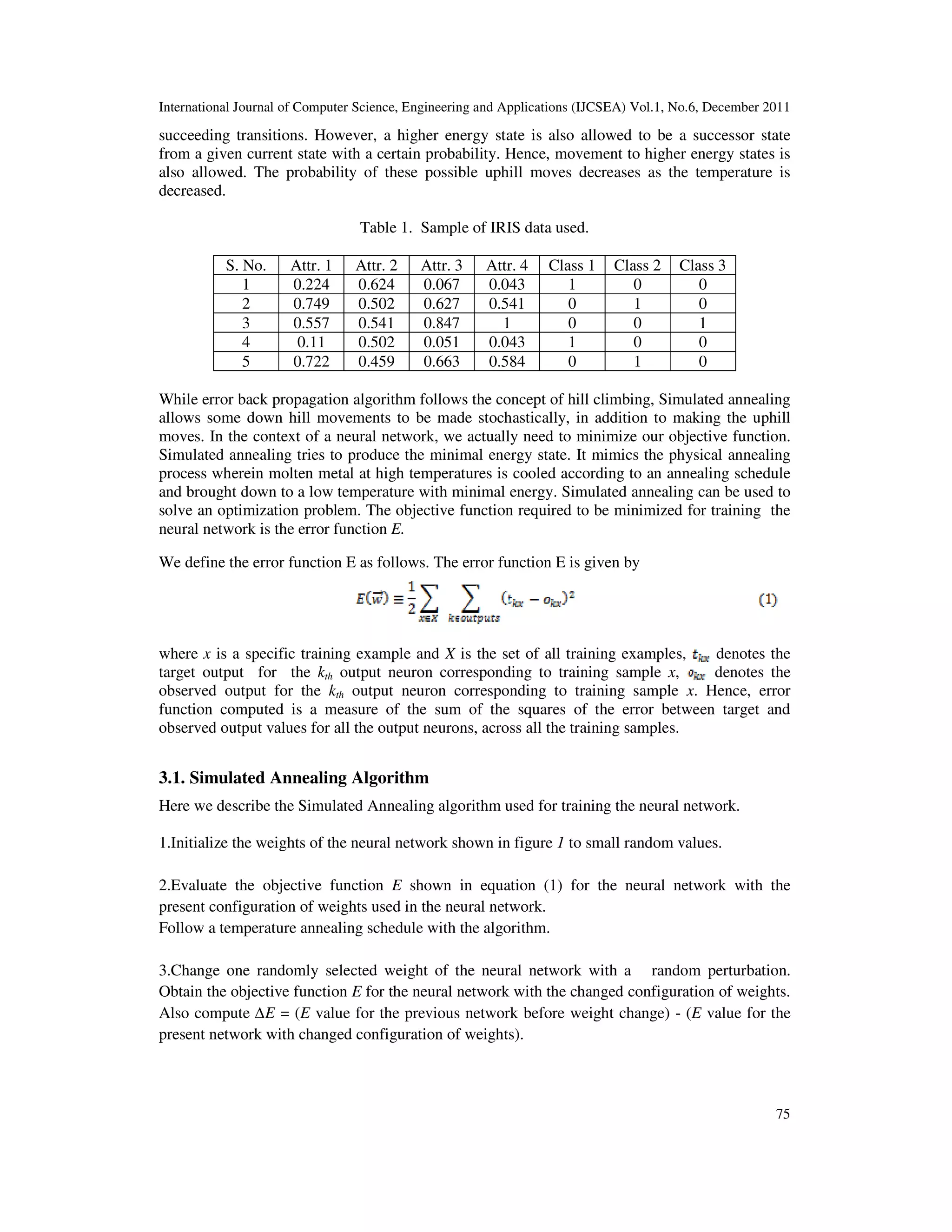
2.1. Iris data
Neural Network shown in figure 1 is used to perform classification task on IRIS data. The data
was taken from the Univ. of California, Irvine (UCI), Machine learning repository. Iris data
consists of 150 input-output vector pairs. Each input vector consists of a 4 tuple having four
attribute values corresponding to the four input attributes respectively. Based on the input vector,
output vector gives class to which it belongs. Each output vector is a 3 tuple and will have a ‘1’ in
first, second or third positions and zeros in rest two positions, thereby indicating the class to
which the input vector being considered belongs. Hence, we use 1-of-n encoding on the output
side for denoting the class value. The data of 150 input-output pairs is divided randomly into two
parts to create the training set and test set respectively. Data from training set is used to train the
neural network and data from the test set is used for test purposes. Few samples of IRIS data are
shown in table 1.
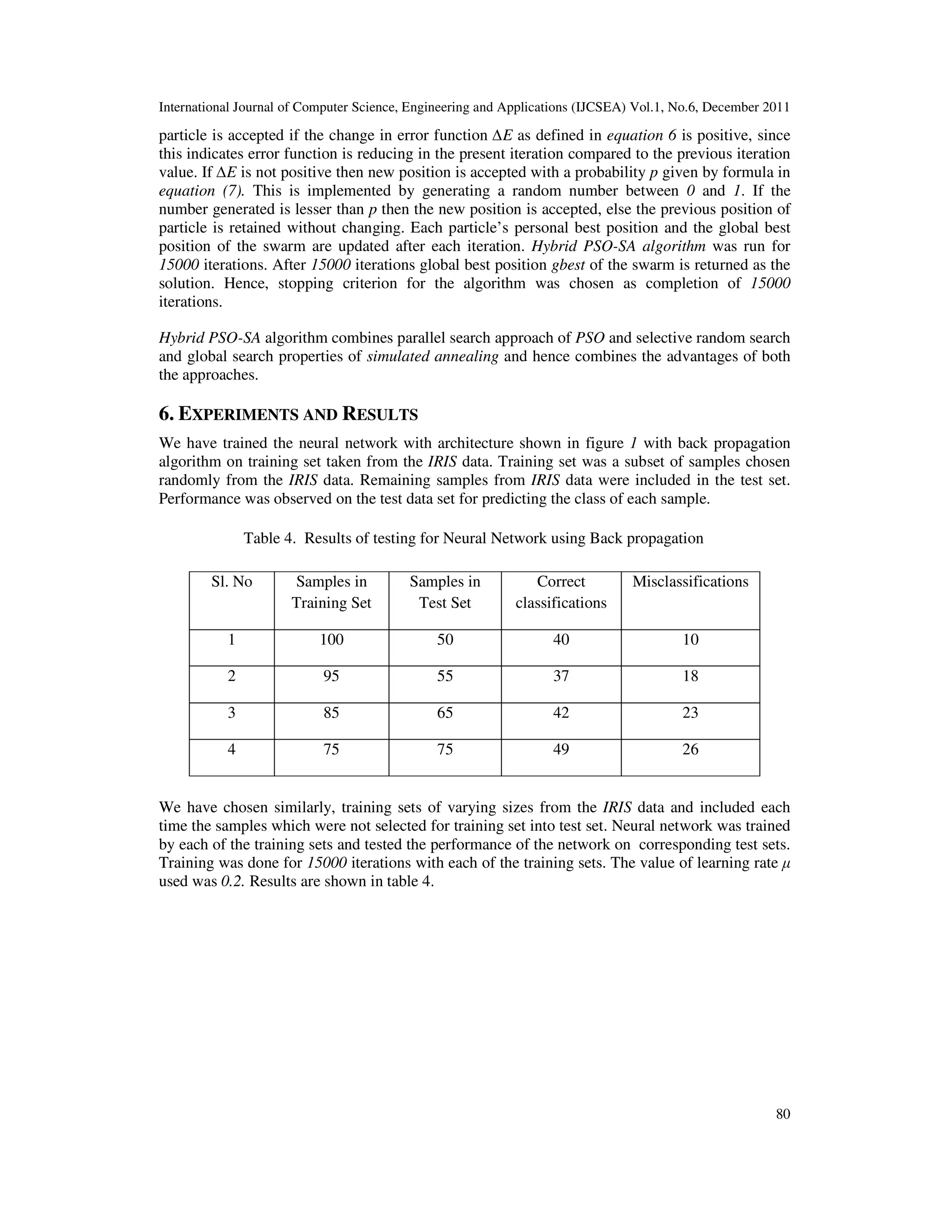
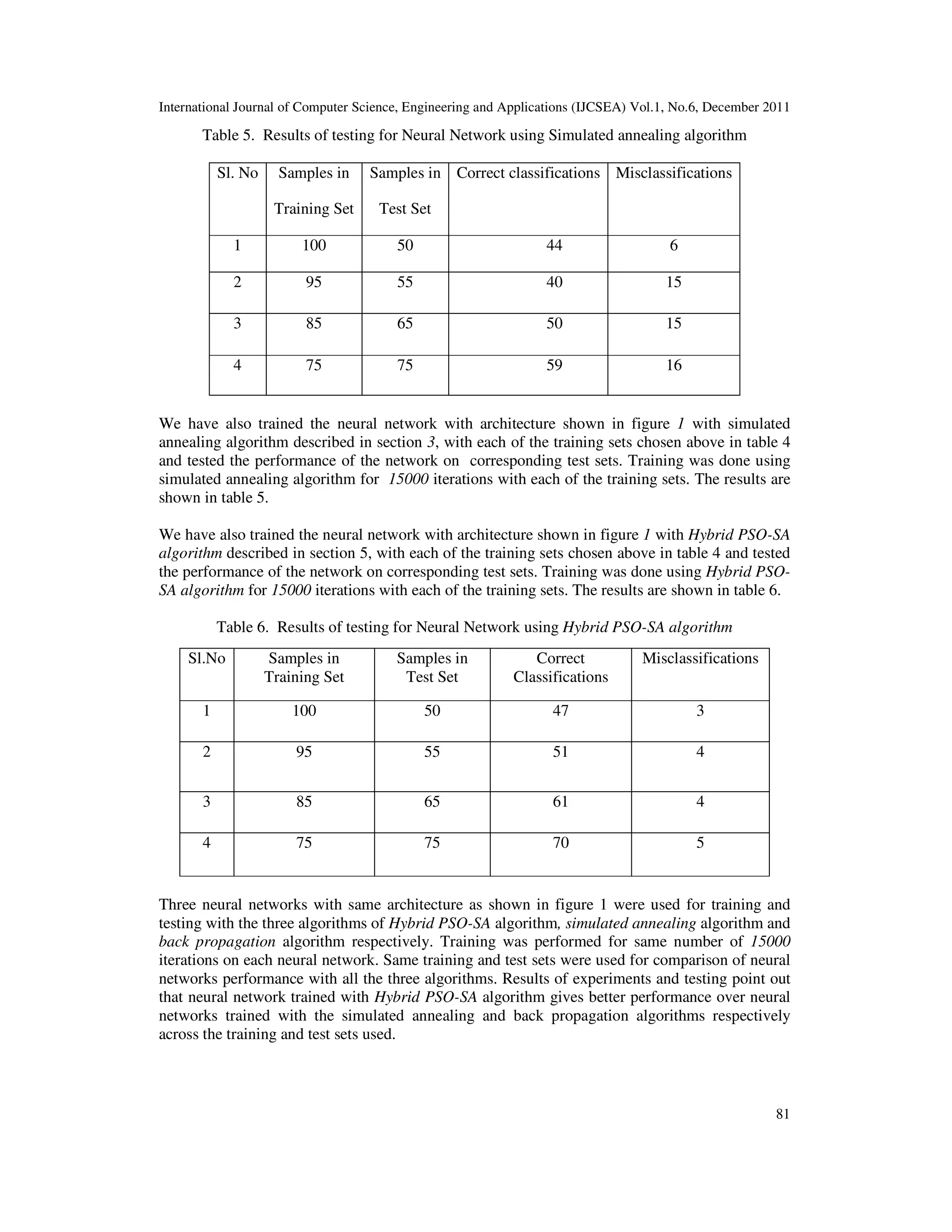
3. SIMULATED ANNEALING TO TRAIN THE NEURAL NETWORK
Simulated annealing [7], [8] was originally proposed as a process which mimics the physical
process of annealing wherein molten metal is cooled gradually from high energy state attained at
high temperatures to low temperature by following an annealing schedule. Annealing schedule
defines how the temperature is gradually decreased. The goal is to make the metal reach a
minimum attainable energy state. In the simulated annealing lower energy states are produced in
Input Hidden Output

75
succeeding transitions. However, a higher energy state is also allowed to be a successor state
from a given current state with a certain probability. Hence, movement to higher energy states is
also allowed. The probability of these possible uphill moves decreases as the temperature is
decreased.
Table 1. Sample of IRIS data used.
S. No. Attr. 1 Attr. 2 Attr. 3 Attr. 4 Class 1 Class 2 Class 3
1 0.224 0.624 0.067 0.043 1 0 0
2 0.749 0.502 0.627 0.541 0 1 0
3 0.557 0.541 0.847 1 0 0 1
4 0.11 0.502 0.051 0.043 1 0 0
5 0.722 0.459 0.663 0.584 0 1 0
While error back propagation algorithm follows the concept of hill climbing, Simulated annealing
allows some down hill movements to be made stochastically, in addition to making the uphill
moves. In the context of a neural network, we actually need to minimize our objective function.
Simulated annealing tries to produce the minimal energy state. It mimics the physical annealing
process wherein molten metal at high temperatures is cooled according to an annealing schedule
and brought down to a low temperature with minimal energy. Simulated annealing can be used to
solve an optimization problem. The objective function required to be minimized for training the
neural network is the error function E.
We define the error function E as follows. The error function E is given by
where x is a specific training example and X is the set of all training examples, denotes the
target output for the kth output neuron corresponding to training sample x, denotes the
observed output for the kth output neuron corresponding to training sample x. Hence, error
function computed is a measure of the sum of the squares of the error between target and
observed output values for all the output neurons, across all the training samples.
3.1. Simulated Annealing Algorithm
Here we describe the Simulated Annealing algorithm used for training the neural network.
1.Initialize the weights of the neural network shown in figure 1 to small random values.
2.Evaluate the objective function E shown in equation (1) for the neural network with the
present configuration of weights used in the neural network.
Follow a temperature annealing schedule with the algorithm.
3.Change one randomly selected weight of the neural network with a random perturbation.
Obtain the objective function E for the neural network with the changed configuration of weights.
Also compute ∆E = (E value for the previous network before weight change) - (E value for the
present network with changed configuration of weights).

76
4.If ∆E is positive then new value of E is smaller and therefore better than previous value. Then
accept the new state and make it the current state. else accept the new state (even though it has a
higher E value) with a probability p defined by
p = ( 2)
5.Revise the temperature T as per schedule defined.
6.Go to step 3 if E value obtained is not yet satisfactory else return solution. Solution is the
present configuration of the weights in the neural network.
3.2 Encoding of the Weights in the Neural Network
The Neural Network in figure 1 has 12 weights between input and hidden layer and 9 weights
between hidden and output layer. So the total number of weights in the network are 21. We coded
these weights in binary form. Each weight was assumed to vary between +12.75 and -12.75 with
a precision of 0.05. This is because weights learned by a typical neural network will be small
positive or negative real numbers. Any real number between -12.75 and +12.75 with a precision
of 0.05 can be represented by a 9-bit binary string. Thus, -12.75 was represented with a binary
string ‘000000000’ and +12.75 was represented with ‘111111111’. For example, number 0.1 is
represented by ‘100000010’. Each of the twenty one weights present in the neural network was
represented by a separate 9 bit binary string and the set of all the weights present in the neural
network is represented by their concatenation having 189 bits. These 189 bits represent one
possible assignment of values to the weights in the neural network.
Initially, a random binary string having 189 bits was generated to make the assignment of weights
randomly for the network. We obtain the value of objective function E for this assignment of
weights to the neural network. Simulated Annealing requires a random perturbation to be given to
the network. We do this by selecting randomly one of the 189 binary bits and flipping it. If the
selected bit was 1 it is changed to 0 and if it was 0 it is changed to 1. For the new configuration of
network with weight change objective function E is calculated. Then, ∆E was calculated as (E
value for the previous network before weight change) - (E value for the present network with
changed configuration of weights). Using this approach, simulated annealing algorithm shown in
section 3.1 was executed following a temperature schedule.
The temperature schedule followed is defined as follows:
The starting temperature is taken as T =1050;
Current temp = T/log(iterations+1);
Current temperature was changed after every 100 iterations using above formula.
4. ERROR BACK-PROPAGATION
Error-Back propagation algorithm uses gradient descent search. Gradient descent approach
searches for the weight vector that minimizes error E. Towards this, it starts from an arbitrary
initial weight vector and then changes it in small steps. At each of these steps the weight is altered
in the direction which produces steepest descent along the error surface. Hence, gradient descent
approach follows the hill climbing approach.
The direction of the steepest descent along the error surface is found by computing the derivative
of E with respect to the weight vector w.
Gradient of E with respect to w is = (3)

77
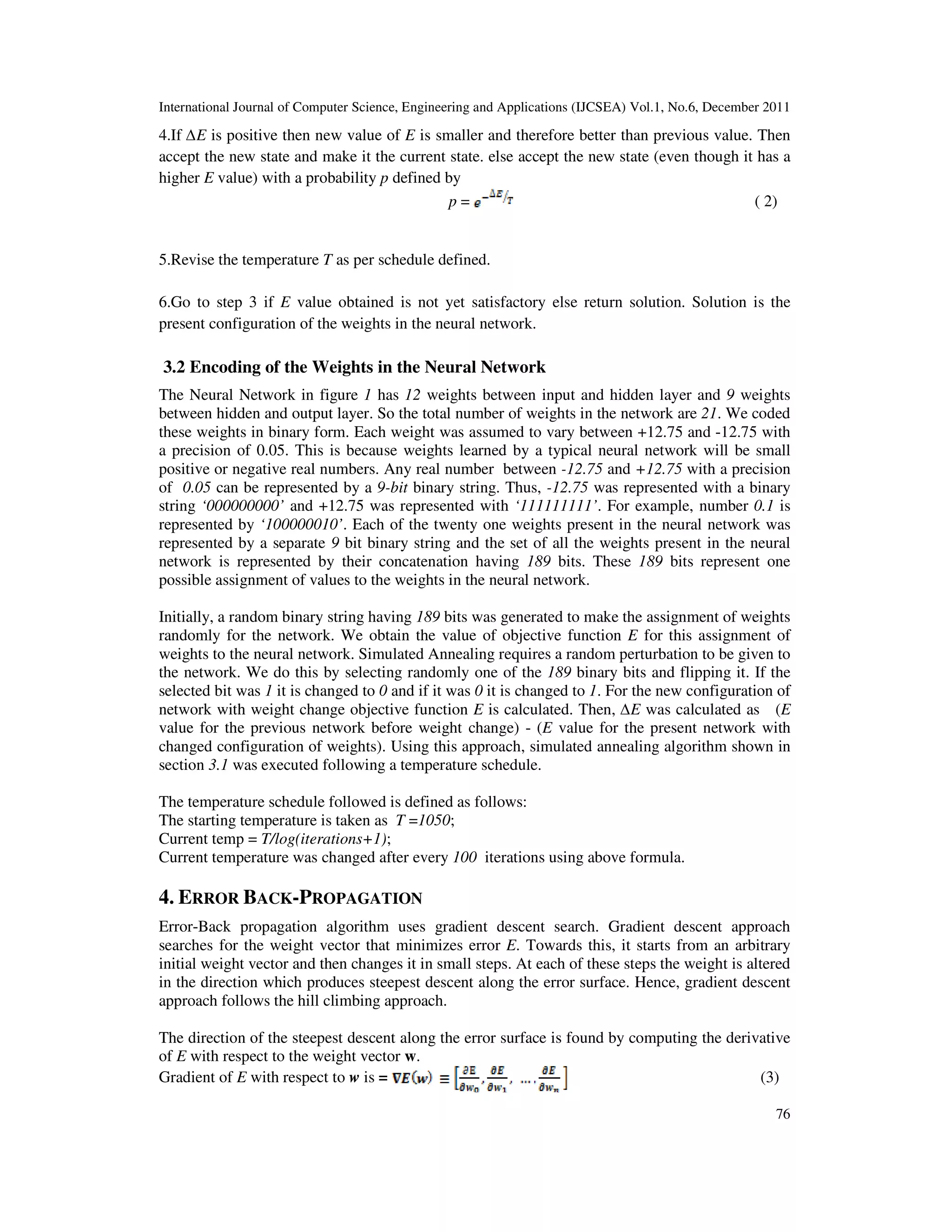
4.1 Algorithm for Back-propagation
Since the back propagation algorithm has been introduced [3], [5] it has been used widely as the
training algorithm for training the weights of the feed forward neural network. It was able to
overcome the limitation faced by the perceptron since it can be used for classification for non-
linearly separable problems unlike perceptron. Perceptron can only solve linearly separable
problems. Main disadvantage of neural network using back propagation algorithm is that since it
uses hill climbing approach it can get stuck at local minima. Below we present in table 2 the back
propagation algorithm [9] for the feed forward neural network. It describes the Back propagation
algorithm using batch update wherein weight updates are computed for each weight in the
network after considering all the training samples in a single iteration or epoch. It takes many
iterations or epochs to complete the training of the neural network.
Table 2. Back propagation Algorithm
Back propagation algorithm
Each training sample is a pair of the form ( ), where x is the input vector, and t is the
target vector.
µ is the learning rate, m is the number of network inputs to the neural network, y is the
number of units in the hidden layer , z is the number of output units.
The input from unit i into unit j is denoted by xji , and the weight from unit i into unit j is
denoted by wji .
● Create a feed-forward network with m inputs, y hidden units, and z output units.
● Initialize all network weights to small random numbers.
● Until the termination condition is satisfied, do
● For each in training samples , do
Propagate the input vector forward through the network:
1. Input the instance to the network and compute the output ou of
every unit u in the network.
Propagate the errors backward through the network:
2. For each network output unit k , with target output calculate its
error term
3. For each hidden unit h, calculate its error term
4. For each network weight , do
● For each network weight , do

78
5. HYBRID PSO-SA ALGORITHM
In particle swarm optimization [11, 12] a swarm of particles are flown through a
multidimensional search space. Position of each particle represents a potential solution. Position
of each particle is changed by adding a velocity vector to it. Velocity vector is influenced by the
experiential knowledge of the particle as well as socially exchanged information. The
experiential knowledge of a particle A describes the distance of the particle A from its own best
position since the particle A’s first time step. This best position of a particle is referred to as the
personal best of the particle. The global best position in a swarm at a time t is the best position
found in the swarm of particles at the time t. The socially exchanged information of a particle A
describes the distance of a particle A from the global best position in the swarm at time t. The
experiential knowledge and socially exchanged information are also referred to as cognitive and
social components respectively. We propose here the hybrid PSO-SA algorithm in table 3.
Table 3. Hybrid Particle swarm optimization-Simulated annealing algorithm
Create a nx dimensional swarm of ns particles;
repeat
for each particle i = 1, . . .,ns do
// yi denotes the personal best position of the particle i so far
// set the personal best position
if f (xi) < f (yi) then
yi = xi ;
end
// ŷ denotes the global best of the swarm so far
// set the global best position
if f (yi) < f ( ŷ ) then
ŷ = yi ;
end
end
for each particle i = 1, . . ., ns do
update the velocity vi of particle i using equation (4);
vi (t+1) = vi (t) + c1 r1 (t)[yi (t) – xi(t) ] + c2 r2 (t)[ŷ (t) – xi(t)] (4)
// where yi denotes the personal best position of the particle i
// and ŷ denotes the global best position of the swarm
// and xi denotes the present position vector of particle i.
update the position using equation (5);
bi(t) = xi (t) //storing present position
xi (t+1) = xi (t) + vi (t+1) (5)
// applying simulated annealing
compute ∆E = (f (xi) - f(xi (t+1)) (6)
// ∆E = (E value for the previous network before weight change) - (E value

79
for the present network with changed configuration of weights).
• if ∆E is positive then
// new value of E is smaller and therefore better than previous value. Then
// accept the new position and make it the current position
else accept the new position xi (t+1) (even though it has a higher E value)
with a probability p defined by
p = (7)
• Revise the temperature T as per schedule defined below.
The temperature schedule followed is defined as follows:
The starting temperature is taken as T =1050;
Current temp = T/log(iterations+1);
Current temperature was changed after every 100 iterations using
above formula.
end
until stopping condition is true ;
In equation (4) of table 3, vi , yi and ŷ are vectors of nx dimensions. vij denotes scalar component
of vi in dimension j. vij is calculated as shown in equation 7 where r1j and r2j are random values in
the range [0,1] and c1 and c2 are learning factors chosen as c1 = c2 = 2.
vij (t+1) = vij (t) + c1 r1j (t)[yij (t) – xij(t) ] + c2 r2j (t)[ŷj (t) – xij) (t)] (8)
5.1 Implementation details of Hybrid PSO-SA algorithm for training a neural
network
We describe here the implementation details of hybrid PSO-SA algorithm for training the neural
network. There are 21 weights in the neural network shown in figure 1.
Hybrid PSO-SA algorithm combines particle swarm optimization algorithm with simulated
annealing approach in the context of training a neural network. The swarm is initialized with a
population of 50 particles. Each particle has 21 weights. Each weight value corresponds to a
position in a particular dimension of the particle. Since there are 21 weights for each particle,
there are therefore 21 dimensions. Hence, position vector of each particle corresponds to a 21
dimensional weight vector. Position (weight) in each dimension is modified by adding velocity
value to it in that dimension.
Each particle’s velocity vector is updated by considering the personal best position of the
particle, global best position of the entire swarm and the present position vector of the particle as
shown in equation (4) of table 3. Velocity of a particle i in dimension j is calculated as shown in
equation (8).
Hybrid PSO-SA algorithm combines pso algorithm with simulated annealing approach. Each of
the 50 particles in the swarm is associated with 21 weights present in the neural network. The
error function E(w) which is a function of the weights in the neural network as defined in
equation (1) is treated as the fitness function. Error E(w) ( fitness function) needs to be
minimized. For each of the 50 particles in the swarm, the solution (position) given by the

80
particle is accepted if the change in error function ∆E as defined in equation 6 is positive, since
this indicates error function is reducing in the present iteration compared to the previous iteration
value. If ∆E is not positive then new position is accepted with a probability p given by formula in
equation (7). This is implemented by generating a random number between 0 and 1. If the
number generated is lesser than p then the new position is accepted, else the previous position of
particle is retained without changing. Each particle’s personal best position and the global best
position of the swarm are updated after each iteration. Hybrid PSO-SA algorithm was run for
15000 iterations. After 15000 iterations global best position gbest of the swarm is returned as the
solution. Hence, stopping criterion for the algorithm was chosen as completion of 15000
iterations.
Hybrid PSO-SA algorithm combines parallel search approach of PSO and selective random search
and global search properties of simulated annealing and hence combines the advantages of both
the approaches.
6. EXPERIMENTS AND RESULTS
We have trained the neural network with architecture shown in figure 1 with back propagation
algorithm on training set taken from the IRIS data. Training set was a subset of samples chosen
randomly from the IRIS data. Remaining samples from IRIS data were included in the test set.
Performance was observed on the test data set for predicting the class of each sample.
Table 4. Results of testing for Neural Network using Back propagation
Sl. No Samples in
Training Set
Samples in
Test Set
Correct
classifications
Misclassifications
1 100 50 40 10
2 95 55 37 18
3 85 65 42 23
4 75 75 49 26
We have chosen similarly, training sets of varying sizes from the IRIS data and included each
time the samples which were not selected for training set into test set. Neural network was trained
by each of the training sets and tested the performance of the network on corresponding test sets.
Training was done for 15000 iterations with each of the training sets. The value of learning rate µ
used was 0.2. Results are shown in table 4.

81
Table 5. Results of testing for Neural Network using Simulated annealing algorithm
Sl. No Samples in
Training Set
Samples in
Test Set
Correct classifications Misclassifications
1 100 50 44 6
2 95 55 40 15
3 85 65 50 15
4 75 75 59 16
We have also trained the neural network with architecture shown in figure 1 with simulated
annealing algorithm described in section 3, with each of the training sets chosen above in table 4
and tested the performance of the network on corresponding test sets. Training was done using
simulated annealing algorithm for 15000 iterations with each of the training sets. The results are
shown in table 5.
We have also trained the neural network with architecture shown in figure 1 with Hybrid PSO-SA
algorithm described in section 5, with each of the training sets chosen above in table 4 and tested
the performance of the network on corresponding test sets. Training was done using Hybrid PSO-
SA algorithm for 15000 iterations with each of the training sets. The results are shown in table 6.
Table 6. Results of testing for Neural Network using Hybrid PSO-SA algorithm
Three neural networks with same architecture as shown in figure 1 were used for training and
testing with the three algorithms of Hybrid PSO-SA algorithm, simulated annealing algorithm and
back propagation algorithm respectively. Training was performed for same number of 15000
iterations on each neural network. Same training and test sets were used for comparison of neural
networks performance with all the three algorithms. Results of experiments and testing point out
that neural network trained with Hybrid PSO-SA algorithm gives better performance over neural
networks trained with the simulated annealing and back propagation algorithms respectively
across the training and test sets used.
Sl.No Samples in
Training Set
Samples in
Test Set
Correct
Classifications
Misclassifications
1 100 50 47 3
2 95 55 51 4
3 85 65 61 4
4 75 75 70 5

82
7. CONCLUSIONS
Our objective was to compare the performance of feed-forward neural network trained with
Hybrid PSO-SA algorithm with the neural networks trained by simulated annealing and back
propagation algorithm respectively. The task we have tested using neural networks trained
separately using these three algorithms is the IRIS data classification. We found that neural
network trained with Hybrid PSO-SA algorithm has given better classification performance
among the three. Neural network trained with Hybrid PSO-SA algorithm combines parallel
search approach of PSO and selective random search and global search properties of simulated
annealing and hence combines the advantages of both the approaches. Hybrid PSO-SA algorithm
has performed better than simulated annealing algorithm using its parallel search strategy with a
swarm of particles. It was able to avoid the local minima by stochastically accepting uphill moves
in addition to the making the normal downhill moves across the error surface. It has given better
classification performance over neural network trained by back-propagation. In general, neural
networks trained by back propagation algorithm are susceptible for falling in local minima.
Hence, Hybrid PSO-SA algorithm has given better results for training a neural network and is a
better alternative to both the Simulated annealing and Back propagation algorithms.
REFERENCES
[1] Quinlan, J.R.(1986). Induction of decision trees. Machine Learning, 1 (1), 81-106.
[2] Mitchell, T.M.(1977). Version spaces: A candidate elimination approach to rule learning. Fifth
International Joint Conference on AI (pp.305-310). Cambridge, MA: MIT Press.
[3] Rumelhart, D.E., & McClelland, J.L.(1986). Parallel distributed processing: exploration in the
microstructure of cognition(Vols.1 & 2). Cambridge, MA : MIT Press.
[4] Duda, R.O., & Hart, P.E.(1973). Pattern classification and scene analysis New York: John Wiley &
Sons.
[5] Werbos, P. (1975). Beyond regression: New tools for prediction and analysis in the behavioral
sciences (Ph.D. dissertation). Harvard University.
[6] Parker, D.(1985). Learning logic (MIT Technical Report TR-47). MIT Center for Research in
Computational Economics and Management Science.
[7] Kirkpatrick, S., Gelatt,Jr., C.D., and M.P. Vecchi 1983. Optimization by simulated annealing. Science
220(4598).
[8] Russel, S., & Norvig, P. (1995). Artificial intelligence: A modern approach. Englewood Cliffs,
NJ:Prentice-Hall.
[9] Mitchell, T.M., 1997.Machine Learning, New York: McGraw-Hill.
[10] Kirkpatrick, S., 1984 “Optimization by simulated annealing: Quantitative Studies,” Journal of
Statistical Physics, vol.34,pp.975-986.
[11] Kennedy, J., Eberhart, R., 1995. “Particle swarm optimization”, IEEE International Conference on
Neural Networks, Perth, WA , (pp.1942 – 1948), Australia.
[12] Engelbrecht, A.P., 2007, Computational Intelligence, England: John Wiley & Sons.

83
Authors
Sriram G. Sanjeevi has B.E. from Osmania University, M.Tech from M.I.T.
Manipal, Mangalore University and PhD from IIT, Bombay. He is currently
Associate Professor & Head of Computer Science & Engineering Dept., NIT
Warangal. His research interests are Neural networks, Machine learning and Soft
computing.
A. N. Nikhila has B.Tech(CSE) from NIT Warangal. Her research interests are Neural networks, Machine
learning.
Thaseem Khan has B.Tech(CSE) from NIT Warangal. His research interests are Neural networks, Machine
learning.
G. Sumathi has B.Tech(CSE) from NIT Warangal. Her research interests are Neural networks, Machine
learning.

Hybrid PSO-SA algorithm for training a Neural Network for Classification

Recommended

Recommended

More Related Content

What's hot

What's hot (19)

Similar to Hybrid PSO-SA algorithm for training a Neural Network for Classification

Similar to Hybrid PSO-SA algorithm for training a Neural Network for Classification (19)

Recently uploaded

Recently uploaded (20)

Hybrid PSO-SA algorithm for training a Neural Network for Classification