This paper presents a new approach for image compression using artificial neural networks and gradient descent technology, addressing issues of haziness in decompressed images at high compression rates. The study compares the performance of genetic algorithms and back propagation, ultimately finding that the back propagation algorithm yields better results for image compression while enhancing data security. The results indicate promising applications of neural network-based compression techniques in various fields.
![The International Journal Of Engineering And Science (IJES)
|| Volume || 3 || Issue || 12 || Pages || 10-17 || 2014 ||
ISSN (e): 2319 – 1813 ISSN (p): 2319 – 1805
www.theijes.com The IJES Page 10
Modeling of neural image compression using gradient decent
technology
Anusha K L1
, Madhura G2
, Lakshmikantha S3
1,
Asst.Prof, Department of CSE,EWIT, Bangalore
2.
Asst.Prof, Department of CSE,EWIT, Bangalore
3.
Asst.Prof, Department of CSE,EWIT, Bangalore
--------------------------------------------------------------ABSTRACT-------------------------------------------------------
In this paper, we introduce a new approach for image compression. At higher compression rate, the
decompressed image gets hazy in GIF and PNG, an image compression technique. In order to overcome from
those problems artificial neural networks can be used. In this paper, gradient decent technology is used to
provide security of stored data. BP provides higher PSNR ratio, with fast rate of learning. Experiments reveal
that gradient decent technology works better than Genetic algorithm where the image gets indistinguishable as
well as not transmitted in a secured manner.
Keywords: Image-compression, back propagation, gradient decent, artificial neural network, genetic
algorithm
---------------------------------------------------------------------------------------------------------------------------------------
Date of Submission: 19 June 2014 Date of Accepted: 20 December 2014
---------------------------------------------------------------------------------------------------------------------------------------
I. INTRODCUTION
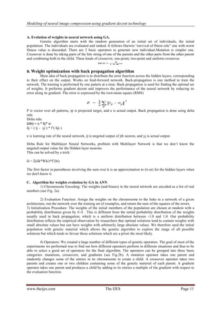
Artificial neural network(ANN) are computational models inspired by animals „central nervous
system‟(particular brain)[5,6,8]which are capable of machine learning and pattern recognition .Like the brain,
this computing model consist of many small units or neurons or node (the circle) are interconnected .There are
several different neural networks models that differ widely in functions and applications. In [1,2,3,4,7 ]paper we
discuss the feed-forward network with back propagation learning .From mathematical view; a feed-forward
neural network is function. It takes an input and produces an output. The input and output are represented by
real numbers. A simple neural network may be illustrated like in Fig.1.
Fig 1: Simple Neural Network
This network consists of 5 units or neurons or nodes (the circle) and 6 connections (the arrows). The
number next to each connection is called weight; it indicates the strength of the connection .Positive weight
excitatory. Negative weight inhibitory. This is a feed forward network, because the connections are directed in
only one way from top to bottom. There are no loops or circles.
II. FEED FORWARD ARTIFICIAL NEURAL NETWORKS
Information processing in neural network. The node receives the weighted activation. First these are
added up (summation). The result is passed through an activation function. The outcome is the activation of the
node. For each of the outgoing connections, this activation value is multiplied with the specific weight and
transferred to the next node. It is important that a threshold function is non-linear. Otherwise a multilayer
network is equivalent to a one layer network. The most applied threshold function is sigmoid.
However, the sigmoid is the most common one. It has some benefits for back propagation learning, the
classical training algorithm for feed forward neural network.](https://image.slidesharecdn.com/c31202010017-150218035404-conversion-gate01/85/Modeling-of-neural-image-compression-using-gradient-decent-technology-1-320.jpg)
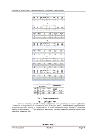
![Modeling of neural image compression using gradient decent technology
www.theijes.com The IJES Page 15
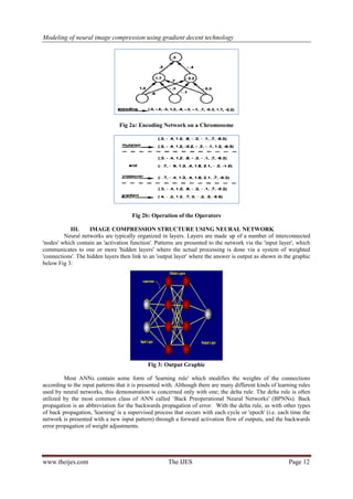
Fig 9: Decompression by GA with ANN
VI. IMAGE COMPRESSION USING ANN AND STANDARD BACK PROPAGATION
ALGORITHM
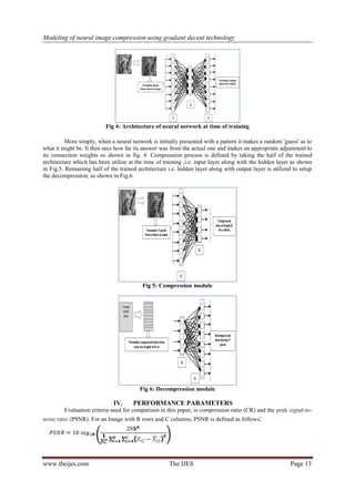
Standard back propagation is one of the most widely used learning algorithms for finding the optimal
set of weights in learning. A single image “Lena” is taken as training data. The error curve of learning is shown
in Fig.10 for below defined set of parameters. Further, different images are tested to generalize the capability of
compression. The processes repeated for two different compression ratios by changing the number of hidden
nodes in neural architecture. The performance observed during the time of training and testing is shown in table
4, table 5 for compression ratio 4:1 and in table 6, table 7 or 8:1, respectively. Table 8 given the comparison
with [9]
Fig 10: Error plot in back propagation
Parameter setting for back propagation learning:
Initial random weights value taken from uniform distribution in range of [-0.0005 +0.0005]. Learning
rate:0.1Momentum constant: 0.5;Bias applied to hidden and output layer nodes with fixed input as (+1).
Allowed number of iteration : 50
Fig 11: Performance by Gradient Decent](https://image.slidesharecdn.com/c31202010017-150218035404-conversion-gate01/85/Modeling-of-neural-image-compression-using-gradient-decent-technology-6-320.jpg)
![Modeling of neural image compression using gradient decent technology
www.theijes.com The IJES Page 17
[1]. J.Jiang, “Image compression with neural networks: A survey”.Signal Processing: Image Communication 14 (1999), 737-760
[2]. Moghadam, R.A. Eslamifar, M. “Image compression using linear and nonlinear principal component neural networks” .Digital
Information and Web Technologies, 2009. ICADIWT „09. Second International Conference on the London, Issue Date: 4-6 Aug.
2009, pp: 855 – 860.
[3]. Palocio, Crespo, Novelle,”image /video compression with artificial neural network”.Springer-Verlag, IWANN 2009, part ii,
LNCS 5518, pp: 330- 337.2009
[4]. Bodyanskiy,grimm,mashtalir,vinarski,”fast training of neural network for image compression”.Springer-Verlag ,ICDM
2010,LNAI 6171, PP;165- 173,2010.
[5]. Liying Ma, Khashayar Khorasani,” Adaptive Constructive Neural Networks Using Hermite Polynomials for Image Compression
“,Advances in Neural Networks, springer, Volume 3497/2005, 713-722, DOI: 10.1007/11427445_115
[6]. Dipta Pratim Dutta, Samrat Deb Choudhury, Md Anwar Hussain, Swanirbhar Majumder, "Digital Image Compression Using
Neural Networks," act, pp.116-120, 2009 International Conference on Advances in Computing, Control, and Telecommunication
Technologies, 2009
[7]. B. Karlik, “Medical Image Compression by Using Vector Quantization Neural Network”, ACAD Sciences press in Computer
Science,vol. 16, no. 4, 2006 pp., 341-348.
[8]. Y. Zhou., C. Zhang, and Z. Zhang, “Improved Variance-Based Fractal Image Compression Using Neural Networks”, Lecture
Notes in Computer Science, Springer-Verlag, vol. 3972, 2006, pp. 575-580](https://image.slidesharecdn.com/c31202010017-150218035404-conversion-gate01/85/Modeling-of-neural-image-compression-using-gradient-decent-technology-8-320.jpg)


![5G Explained! A High Level Overview [Introduction]](https://cdn.slidesharecdn.com/ss_thumbnails/5gexplainedahighleveloverview-260119165306-cc137a3e-thumbnail.jpg?width=640&height=640&fit=bounds)


