The document discusses descriptive statistics such as the mean, median, variance and standard deviation. It uses examples of birth weight data from 5 newborn babies to illustrate how to calculate these statistics. The mean birth weight was 3.68 kg. The standard deviation describes how much the weights vary around the mean. But the sample mean itself has some error since it is based on a subset of data. This error is quantified by the standard error of the mean, which depends on the sample size and standard deviation.

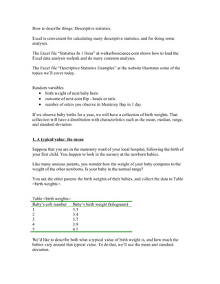
1. How to describe things: Descriptive statistics.
Excel is convenient for calculating many descriptive statistics, and for doing some
analyses.
The Excel file “Statistics In 1 Hour” at walkerbioscience.com shows how to load the
Excel data analysis toolpak and do many common analyses.
The Excel file “Descriptive Statistics Examples” at the website illustrates some of the
topics we’ll cover today.
Random variables
• birth weight of next baby born
• outcome of next coin flip - heads or tails
• number of otters you observe in Monterey Bay in 1 day.
If we observe baby births for a year, we will have a collection of birth weights. That
collection will have a distribution with characteristics such as the mean, median, range,
and standard deviation.
1. A typical value: the mean
Suppose that you are in the maternity ward of your local hospital, following the birth of
your first child. You happen to look in the nursery at the newborn babies.
Like many anxious parents, you wonder how the weight of your baby compares to the
weight of the other newborns. Is your baby in the normal range?
You ask the other parents the birth weights of their babies, and collect the data in Table
<birth weights>.
Table <birth weights>.
Baby’s crib number Baby’s birth weight (kilograms)
1
3.3
2
3.4
3
3.7
4
3.9
5
4.1
We’d like to describe both what a typical value of birth weight is, and how much the
babies vary around that typical value. To do that, we’ll use the mean and standard
deviation.

2. The mean of a group of numbers gives us an idea of a typical value.
If you have N numbers, add up all the N numbers and divide by N. For the five birth
weights in Table <birth weights>, N is 5.
The sum of all 5 numbers is 18.4, so the mean birth weight is 18.4/5 = 3.68 kg:
Mean birth weight = X
= (3.3+ 3.4+ 3.7+ 3.9+ 4.1) / 5
= 18.4/5
= 3.68 kg.
Notice that we use an X with a bar over the top, X , as the symbol for the mean.
You might be interested in comparing the birth weight of your baby to the birth weights
of the other babies, to see if your baby is near the typical weight, or is much above or
below typical weights for newborn babies.
We could describe the variability of the birth weights by giving the highest and the
lowest values (the range of values). But the range is not a very good descriptor of
variability, because it can be greatly affected by a single unusual point. For example a
pre-mature baby might have very low birth weight, which would greatly increase the
range and the apparent variability. The most widely used descriptors of variability are the
variance and the standard deviation.
2 Adding things up: Sigma (Σ) notation
Before we look at variance and the standard deviation, it will be useful to have some
shorthand notation for adding up a set of numbers without having to write them all out.
The notation we’ll use is the Greek symbol Sigma (Σ) When we see Σ it means to take
the sum.
Let’s look again at calculating the mean of the baby’s weights, but now we’ll use sigma
notation. There were 5 babies, and we could assign each of them a label:
Baby’s crib number
X1
X2
X3
X4
X5
Baby’s birth weight (kilograms)
3.3
3.4
3.7
3.9
4.1
The letter X represents the variable, in this case birth weight, and the subscripts 1 through
5 indicate which baby we are considering. We use the annotation Xi (X sub i) to indicate

3. any individual baby without specifying which one. So, if i=2, then we are considering
baby X2, whose birth weight is 3.4 kg.
To indicate that we are adding up the 5 birth weights, we could write as follows.
Sum of 5 birthweights = 3.3+ 3.4+ 3.7+ 3.9+ 4.1.
Or we could write:
Sum of 5 birthweights = X1+ X2+ X3+ X4+ X5.
It would get tedious to write out this formula, so instead we use the notation:
Sum of 5 birthweights
5
=∑Xi
i =1
= sum of Xi for i from1 to 5
= X1+ X2+ X3+ X4+ X5
= 3.3+ 3.4+ 3.7+ 3.9+ 4.1
= 18.4
Sometimes we won’t write out the subscript “i=1” or the superscript “5” if the meaning is
clear. In that case, we might just write ΣXi .
Finally, to calculate the mean of the 5 birthweights using sigma notation, we write the
following.
Mean of 5 birthweights = X
5
=∑Xi
i =1
5
= 3.68
Notice again that the symbol for the mean is X-bar, X .
3. Descriptors of variability: variance and standard deviation
We can describe variability of a group, such as the five babies, using the variance, which
we define as follows. The symbol for variance is σ2, sigma squared.
Population variance = σ2

4. N
(
∑ X i− X
i =1
)2
N
=
= [(3.3 – 3.68)2 + (3.4– 3.68) 2 + (3.7– 3.68) 2 + (3.9– 3.68) 2 + (4.1– 3.68) 2] /5
= 0.448 kg2/5
= 0.0896 kg2
Notice that the variance has units of kg2, kilograms squared. We’d like to have a measure
of variability in kilograms, the same units as the original measurements. A measure of
variability in the same units as the original measurements is the standard deviation, σ,
sigma. The standard deviation, σ, is the square root of the variance, σ2.
Population standard deviation = Square root (population variance)
= square root (σ2)
=σ
= square root (0. 0896 kg2)
= 0.299 kg.
Notice that we’ve used the terms population variance and population standard deviation.
If we are only interested in these 5 babies, and not in any other babies, then these 5 are
our entire population.
Alternatively, we may be interested in information about all of the babies that are in the
hospital in a given year. In that case, these 5 babies are just a sample of the babies that
are in the hospital in a given year.
Take a random sample from a population
n = number of observations in the sample.
Sample variance and the Sample standard deviation much as we do for the population,
with a small change.
For the population variance, we divide by N, while for the sample variance we divide by
N-1. Thus, the sample variance is slightly larger than the population variance.
Sample variance = S2
N
2
∑ X i− X
i =1
=
(
)
N −1

5. = [(3.3 – 3.68)2 + (3.4– 3.68)2 + (3.7– 3.68)2 + (3.9– 3.68)2 + (4.1– 3.68)2/(5-1)
= (0.448 kg2)/4
= 0.112 kg2
Notice that the sample variance has its own symbol, S2. The sample standard deviation, S,
is the square root of the sample variance, S2.
Sample standard deviation = S
= Square root (sample variance)
= Square root (S2)
= Square root (0.112)
= 0.335 kg.
Most software programs, including Excel, give you the sample variance and sample
standard deviation by default.
4. How well can we estimate the mean? Standard Error of the Mean (SEM)
Suppose we want to evaluate a drug to treat blood pressure.
•
Give to one patient. BP is 2 units lower. Effective?
•
Give to two patients. Mean BP is 3 units lower. Effective?
How can we be confident that the drug is better than placebo?
Let’s do a thought experiment. The 5 babies we looked at the day that we were in the
hospital were only a small fraction of all the babies that might be in the maternity ward in
a year. Their mean birth weight is 3.68 kg.
If we took a different sample of 5 babies from the same hospital on another day, would
their mean birth weight also be exactly 3.68 kg?
Most likely, it would be a little higher or a little lower than 3.68 kg.
The mean birth weight for any given sample, which contains only part of the whole
population, is an estimate of the population mean, and will likely be a little different from
the true population mean.
The difference between the population mean and the sample mean is the error in
estimating the population mean.

6. If we take many samples from the population, we will get many different estimates of the
population mean.
The sample mean is a statistic; the value of the sample mean depends on which
observations are included in the random sample.
So the sample mean is itself a random variable. It has its own mean and standard
deviation.
The average of the set of sample means is equal to the population mean (Law of large
numbers)
The standard deviation of the set of sample means is equal to the standard deviation of
the population divided by the square root of n, where n is the number of observations in
the sample (Central Limit Theorem). Provided n is sufficiently large, the Central Limit
Theorem tells us that the sampling distribution of the mean is asymptotically normal.
The standard deviation of the sample mean has a special name: the standard error of the
mean (SEM).
We can estimate how close the mean for a given sample is to the population mean using
the Standard Error of the Mean (SEM). The symbol for SEM is σ X . We calculate SEM
as follows.
Standard Error of the Mean = SEM = σ X
= (Population standard deviation)/(Square root of N)
However, we usually don’t know the population standard deviation, σ, so instead we use
the sample standard deviation, s. Because they differ only in the denominator being N
versus N-1, it makes little difference which we use when N is sufficiently large.
So, for a single sample from a population, we estimate SEM as follows using the sample
standard deviation.
Standard Error of the Mean = SEM
= (Sample standard deviation)/(Square root of N)
s
=
N
For our baby example, we calculate SEM as follows.
Sample standard deviation = s = .335
N=5

7. Standard Error of the Mean = SEM
0.335
5
=
= 0.1497
The SEM depends on both the sample standard deviation, S and of the number of
observations in our sample, N.
Not surprisingly, the more observations N we have in our sample, the better our estimate
of the population mean.
If we only have N = 1 or N = 2, we’re not very confident about the population mean.
On the other hand, if we have N = 100 or N = 1000, we start to be a lot more confident
that the mean of the sample is close to the population mean.
If the population has very small variability, giving us a small sample standard deviation,
then most samples will be pretty tightly clustered around the population mean, and a
small SEM.
If the population has high variability, giving us a large standard deviation, then samples
may be scattered widely, giving us a large SEM.
We’ll use SEM in statistical tests such as t-tests and analysis of variance to compare
groups.
The concept of the standard error of a statistic (such as the standard error of the sample
mean, or the standard error of coefficients in a regression model) is critical to
determining the significance of the statistic.

8. Extra topic 1. Robust descriptors, median, rank and non-parametric tests
The mean of a group can be greatly affected by a single extreme value. Suppose we
calculate the average income of all the people in Redmond, Washington, the headquarters
of Microsoft. The mean is going to be greatly affected by the income of Bill Gates, and
may not give us a very representative idea about the income of a typical person working
in Redmond. An alternative way to describe the typical income is the median, which is
the middle observation in a set of observations (if there are an odd number of
observations) or the average of the two middle observations (if there are an even number
of observations). For the birth weight example, we had 5 observations, so the middle
observation is the 3rd observation, so the median, is the value of the 3rd observation,
which is 3.7 kg.
Table <birth weights with a single extreme value> shows the same birth weights, but now
the 5th baby has a weight of 6.0 kg. This single baby changes the mean for the sample
from 3.68 kg to 4.06 kg, which is greater than the weight of all the other babies, and thus
is not really very representative. By contrast, the median is unchanged at 3.7 kg.
Table <birth weights with a single extreme value>.
Baby’s crib number Baby’s birth weight (kilograms)
1
3.3
2
3.4
3
3.7
4
3.9
5
6.0
The median is an example of a robust statistic, which means it is affected relatively little
by extreme values. The median depends on the relative rank (order) of the observations.
Many standard statistical tests, such as the t-test we'll see shortly, use the mean, so they
may be affected by extreme values. For most of these tests, there are alternative statistical
tests based on ranks, and these alternative tests are often called non-parametric tests.
Extra topic 2. Variability versus typical value: Coefficient of Variation (CV)
We often are concerned with the magnitude of variability versus the magnitude of a
typical value (the mean). We describe this ratio of variability to typical value using the
coefficient of variation (CV):
Coefficient of variation = CV = (Sample standard deviation)/Mean.
In most laboratory and manufacturing situations, we’d like the variability to be small
compared to the mean value, so a small CV is desirable.

9. Extra topic 3. Representing values on a standardized scale: the z-score
It is sometimes useful to describe an observation in terms of the number of standard
deviations it is from the mean. This measure of distance from the mean is called the zscore and is defined as follows.
z-score = (Xi – X )/S
We can calculate the z-score of each observation in the birth weight data.
Table <z-scores of birth weights>.
Baby’s crib
Baby’s birth weight
number
(kilograms)
1
3.3
2
3.4
3
3.7
4
3.9
5
4.1
z-score
-1.13
-0.83
0.06
0.65
1.25
Extra topic 4. Are error bars on graphs SEM's or Standard deviations?
Graphs often show a mean value for a variable (such as birth weight) along with error
bars. Unfortunately, the graph often fails to tell you what the error bars mean. Does an
error bar represent one standard deviation? Two standard deviations? One SEM? Two
SEM’s? Without this information, it is easy to be mislead into thinking that two groups
are almost the same (if the error bars represent two standard deviations) or completely
different (if the error bars represent one SEM). If someone shows you a graph with error
bars, ask what they mean.

10. Extra topic 3. Representing values on a standardized scale: the z-score
It is sometimes useful to describe an observation in terms of the number of standard
deviations it is from the mean. This measure of distance from the mean is called the zscore and is defined as follows.
z-score = (Xi – X )/S
We can calculate the z-score of each observation in the birth weight data.
Table <z-scores of birth weights>.
Baby’s crib
Baby’s birth weight
number
(kilograms)
1
3.3
2
3.4
3
3.7
4
3.9
5
4.1
z-score
-1.13
-0.83
0.06
0.65
1.25
Extra topic 4. Are error bars on graphs SEM's or Standard deviations?
Graphs often show a mean value for a variable (such as birth weight) along with error
bars. Unfortunately, the graph often fails to tell you what the error bars mean. Does an
error bar represent one standard deviation? Two standard deviations? One SEM? Two
SEM’s? Without this information, it is easy to be mislead into thinking that two groups
are almost the same (if the error bars represent two standard deviations) or completely
different (if the error bars represent one SEM). If someone shows you a graph with error
bars, ask what they mean.