INTRODUCTION TO EMBEDDED SYSTEMSA CYBER-PHYS.docx

IN
TRODUCTION
TO
EM
BEDDED SYSTEM
S
A CYBER-PHYSICAL
SYSTEM
S APPROACH
Edw
ard Ashford Lee and
Sanjit Arunkum
ar Seshia
computer science/electrical engineering
Introduction to Embedded Systems
A Cyber-Physical Systems Approach
second edition
Edward Ashford Lee and Sanjit Arunkumar Seshia
The most visible use of computers and software is processing
information for human consumption. The vast majority
of computers in use, however, are much less visible. They run
the engine, brakes, seatbelts, airbag, and audio system
in your car. They digitally encode your voice and construct a

radio signal to send it from your cell phone to a base sta-
tion. They command robots on a factory floor, power generation
in a power plant, processes in a chemical plant, and
traffic lights in a city. These less visible computers are called
embedded systems, and the software they run is called
embedded software. The principal challenges in designing and
analyzing embedded systems stem from their interac-
tion with physical processes. This book takes a cyber-physical
approach to embedded systems, introducing the engi-
neering concepts underlying embedded systems as a technology
and as a subject of study. The focus is on modeling,
design, and analysis of cyber-physical systems, which integrate
computation, networking, and physical processes.
The second edition offers two new chapters, several new
exercises, and other improvements. The book can be
used as a textbook at the advanced undergraduate or
introductory graduate level and as a professional reference
for practicing engineers and computer scientists. Readers should
have some familiarity with machine structures,
computer programming, basic discrete mathematics and
algorithms, and signals and systems.
Edward Ashford Lee is the Robert S. Pepper Distinguished
Professor in the Department of Electrical Engineering and
Computer Sciences at the University of California, Berkeley.
Sanjit Arunkumar Seshia is a Professor in the Depart-
ment of Electrical Engineering and Computer Sciences at the
University of California, Berkeley.
“Books titled Introduction to Embedded Systems traditionally
focus on computer hardware and software. By taking
A Cyber-Physical Systems Approach, Lee and Seshia give
students the integrated perspective they need to under-
stand and design the computing systems that make our world
function. No other book provides such a comprehen-
sive introduction to embedded systems for real-time

applications.”
—Bruce H. Krogh, Professor of Electrical and Computer
Engineering, Carnegie Mellon University
“Introduction to Embedded Systems by Lee and Seshia is an
introductory yet rigorous textbook for the future Internet
of Things engineer. It provides a unified systems view of
computing and the physical world that will be the foundation
of the 21st-century Internet of Things revolution.”
—George J. Pappas, Joseph Moore Professor, University of
Pennsylvania
“Designers of embedded systems are only too often
overwhelmed by the many skills and disciplines that have to be
mastered: from writing device drivers, to worst case execution
time analysis, to formal verification and modeling of
continuous time systems. This book by Lee and Seshia is an
excellent guide to bringing order into these complex-
ities of design by discerning the fundamental from the detail,
the essential property from the accidental aspect. It
presents all the indispensable knowledge areas for an embedded
systems designer and leaves out what can be
delegated to other specialized disciplines.”
—Axel Jantsch, Professor of Systems on Chips, Institute of
Computer Technology, TU Wien, Vienna; author of Mod-
eling Embedded Systems and SoC’s
“The outstanding property of this textbook is the combination of
mathematical rigor and comprehensiveness. It is
presented with numerous examples and with such quality that
understanding the material is easy. Introduction to
Embedded Systems is a must-read for those wanting to master
the complexity of what is today the key enabling
technology in most every complex system surrounding us:
embedded and cyber-physical systems.”
—Werner Damm, Director, Interdisciplinary Research Center on
Cooperative Critical Systems, Carl von Ossietzky

University of Oldenburg
The MIT Press
Massachusetts Institute of Technology
Cambridge, Massachusetts 02142
http://mitpress.mit.edu 9 780262 533812
90000
978-0-262-53381-2
second edition
INTRODUCTION TO
EMBEDDED SYSTEMS
A CYBER-PHYSICAL SYSTEMS
APPROACH
Second Edition
Edward Ashford Lee and
Sanjit Arunkumar Seshia
Modeling
Design
Analysis
Copyright c© 2017
Edward Ashford Lee & Sanjit Arunkumar Seshia
This work is licensed under a Creative Commons
Attribution-NonCommercial-NoDerivatives 4.0 International

License.
Second Edition, Version 2.2
ISBN: 978-0-262-53381-2
Please cite this book as:
E. A. Lee and S. A. Seshia,
Introduction to Embedded Systems - A Cyber-Physical Systems
Approach,
Second Edition, MIT Press, 2017.
This book is dedicated to our families.
Contents
Preface . . . . . . . . . . . . . . . . . . . . . . . . . . . . . . . . . . . . . . x
1 Introduction 1
1.1 Applications . . . . . . . . . . . . . . . . . . . . . . . . . . . . . . . . . 2
1.2 Motivating Example . . . . . . . . . . . . . . . . . . . . . . . . . . . . 6
1.3 The Design Process . . . . . . . . . . . . . . . . . . . . . . . . . . . . .
9
1.4 Summary . . . . . . . . . . . . . . . . . . . . . . . . . . . . . . . . . . 16
I Modeling Dynamic Behaviors 17

2 Continuous Dynamics 18
2.1 Newtonian Mechanics . . . . . . . . . . . . . . . . . . . . . . . . . . . .
19
2.2 Actor Models . . . . . . . . . . . . . . . . . . . . . . . . . . . . . . . . 24
2.3 Properties of Systems . . . . . . . . . . . . . . . . . . . . . . . . . . . .
28
2.4 Feedback Control . . . . . . . . . . . . . . . . . . . . . . . . . . . . . .
31
2.5 Summary . . . . . . . . . . . . . . . . . . . . . . . . . . . . . . . . . . 37
Exercises . . . . . . . . . . . . . . . . . . . . . . . . . . . . . . . . . . . . . 38
CONTENTS
3 Discrete Dynamics 42
3.1 Discrete Systems . . . . . . . . . . . . . . . . . . . . . . . . . . . . . .
43
3.2 The Notion of State . . . . . . . . . . . . . . . . . . . . . . . . . . . . .
48
3.3 Finite-State Machines . . . . . . . . . . . . . . . . . . . . . . . . . . . .
48
3.4 Extended State Machines . . . . . . . . . . . . . . . . . . . . . . . . . .
60
3.5 Nondeterminism . . . . . . . . . . . . . . . . . . . . . . . . . . . . . . 64

3.6 Behaviors and Traces . . . . . . . . . . . . . . . . . . . . . . . . . . . .
68
3.7 Summary . . . . . . . . . . . . . . . . . . . . . . . . . . . . . . . . . . 71
Exercises . . . . . . . . . . . . . . . . . . . . . . . . . . . . . . . . . . . . . 73
4 Hybrid Systems 78
4.1 Modal Models . . . . . . . . . . . . . . . . . . . . . . . . . . . . . . . .
79
4.2 Classes of Hybrid Systems . . . . . . . . . . . . . . . . . . . . . . . . .
82
4.3 Summary . . . . . . . . . . . . . . . . . . . . . . . . . . . . . . . . . . 100
Exercises . . . . . . . . . . . . . . . . . . . . . . . . . . . . . . . . . . . . . 102
5 Composition of State Machines 109
5.1 Concurrent Composition . . . . . . . . . . . . . . . . . . . . . . . . . .
111
5.2 Hierarchical State Machines . . . . . . . . . . . . . . . . . . . . . . .
. 126
5.3 Summary . . . . . . . . . . . . . . . . . . . . . . . . . . . . . . . . . . 130
Exercises . . . . . . . . . . . . . . . . . . . . . . . . . . . . . . . . . . . . . 132
6 Concurrent Models of Computation 135
6.1 Structure of Models . . . . . . . . . . . . . . . . . . . . . . . . . . . . .
137

6.2 Synchronous-Reactive Models . . . . . . . . . . . . . . . . . . . . . .
. 141
6.3 Dataflow Models of Computation . . . . . . . . . . . . . . . . . . . .
. . 147
6.4 Timed Models of Computation . . . . . . . . . . . . . . . . . . . . . .
. 162
6.5 Summary . . . . . . . . . . . . . . . . . . . . . . . . . . . . . . . . . . 167
Exercises . . . . . . . . . . . . . . . . . . . . . . . . . . . . . . . . . . . . . 172
Lee & Seshia, Introduction to Embedded Systems v
http://LeeSeshia.org
CONTENTS
II Design of Embedded Systems 178
7 Sensors and Actuators 179
7.1 Models of Sensors and Actuators . . . . . . . . . . . . . . . . . . . .
. . 181
7.2 Common Sensors . . . . . . . . . . . . . . . . . . . . . . . . . . . . . .
195
7.3 Actuators . . . . . . . . . . . . . . . . . . . . . . . . . . . . . . . . . . 200
7.4 Summary . . . . . . . . . . . . . . . . . . . . . . . . . . . . . . . . . . 206
Exercises . . . . . . . . . . . . . . . . . . . . . . . . . . . . . . . . . . . . . 207

8 Embedded Processors 210
8.1 Types of Processors . . . . . . . . . . . . . . . . . . . . . . . . . . . . .
211
8.2 Parallelism . . . . . . . . . . . . . . . . . . . . . . . . . . . . . . . . . 220
8.3 Summary . . . . . . . . . . . . . . . . . . . . . . . . . . . . . . . . . . 236
Exercises . . . . . . . . . . . . . . . . . . . . . . . . . . . . . . . . . . . . . 238
9 Memory Architectures 239
9.1 Memory Technologies . . . . . . . . . . . . . . . . . . . . . . . . . . .
240
9.2 Memory Hierarchy . . . . . . . . . . . . . . . . . . . . . . . . . . . . .
242
9.3 Memory Models . . . . . . . . . . . . . . . . . . . . . . . . . . . . . . .
251
9.4 Summary . . . . . . . . . . . . . . . . . . . . . . . . . . . . . . . . . . 256
Exercises . . . . . . . . . . . . . . . . . . . . . . . . . . . . . . . . . . . . . 257
10 Input and Output 260
10.1 I/O Hardware . . . . . . . . . . . . . . . . . . . . . . . . . . . . . . . .
261
10.2 Sequential Software in a Concurrent World . . . . . . . . . . . .
. . . . 272
10.3 Summary . . . . . . . . . . . . . . . . . . . . . . . . . . . . . . . . . .
283

Exercises . . . . . . . . . . . . . . . . . . . . . . . . . . . . . . . . . . . . . 284
11 Multitasking 291
11.1 Imperative Programs . . . . . . . . . . . . . . . . . . . . . . . . . . . .
294
11.2 Threads . . . . . . . . . . . . . . . . . . . . . . . . . . . . . . . . . . .
298
vi Lee & Seshia, Introduction to Embedded Systems
CONTENTS
11.3 Processes and Message Passing . . . . . . . . . . . . . . . . . . . .
. . . 311
11.4 Summary . . . . . . . . . . . . . . . . . . . . . . . . . . . . . . . . . .
316
Exercises . . . . . . . . . . . . . . . . . . . . . . . . . . . . . . . . . . . . . 318
12 Scheduling 322
12.1 Basics of Scheduling . . . . . . . . . . . . . . . . . . . . . . . . . . . .
323
12.2 Rate Monotonic Scheduling . . . . . . . . . . . . . . . . . . . . . . .
. 329
12.3 Earliest Deadline First . . . . . . . . . . . . . . . . . . . . . . . . . . .
334

12.4 Scheduling and Mutual Exclusion . . . . . . . . . . . . . . . . . . .
. . 339
12.5 Multiprocessor Scheduling . . . . . . . . . . . . . . . . . . . . . . . .
. 344
12.6 Summary . . . . . . . . . . . . . . . . . . . . . . . . . . . . . . . . . .
348
Exercises . . . . . . . . . . . . . . . . . . . . . . . . . . . . . . . . . . . . . 351
III Analysis and Verification 357
13 Invariants and Temporal Logic 358
13.1 Invariants . . . . . . . . . . . . . . . . . . . . . . . . . . . . . . . . . .
359
13.2 Linear Temporal Logic . . . . . . . . . . . . . . . . . . . . . . . . . .
. 362
13.3 Summary . . . . . . . . . . . . . . . . . . . . . . . . . . . . . . . . . .
370
Exercises . . . . . . . . . . . . . . . . . . . . . . . . . . . . . . . . . . . . . 372
14 Equivalence and Refinement 376
14.1 Models as Specifications . . . . . . . . . . . . . . . . . . . . . . . . .
. 377
14.2 Type Equivalence and Refinement . . . . . . . . . . . . . . . . . .
. . . 378
14.3 Language Equivalence and Containment . . . . . . . . . . . . . .
. . . . 381

14.4 Simulation . . . . . . . . . . . . . . . . . . . . . . . . . . . . . . . . . .
387
14.5 Bisimulation . . . . . . . . . . . . . . . . . . . . . . . . . . . . . . . . .
395
14.6 Summary . . . . . . . . . . . . . . . . . . . . . . . . . . . . . . . . . .
398
Exercises . . . . . . . . . . . . . . . . . . . . . . . . . . . . . . . . . . . . . 399
Lee & Seshia, Introduction to Embedded Systems vii
CONTENTS
15 Reachability Analysis and Model Checking 404
15.1 Open and Closed Systems . . . . . . . . . . . . . . . . . . . . . . . .
. 405
15.2 Reachability Analysis . . . . . . . . . . . . . . . . . . . . . . . . . . .
. 406
15.3 Abstraction in Model Checking . . . . . . . . . . . . . . . . . . . .
. . . 413
15.4 Model Checking Liveness Properties . . . . . . . . . . . . . . . .
. . . . 417
15.5 Summary . . . . . . . . . . . . . . . . . . . . . . . . . . . . . . . . . .
423

Exercises . . . . . . . . . . . . . . . . . . . . . . . . . . . . . . . . . . . . . 425
16 Quantitative Analysis 427
16.1 Problems of Interest . . . . . . . . . . . . . . . . . . . . . . . . . . . .
. 428
16.2 Programs as Graphs . . . . . . . . . . . . . . . . . . . . . . . . . . . . .
430
16.3 Factors Determining Execution Time . . . . . . . . . . . . . . . .
. . . . 435
16.4 Basics of Execution Time Analysis . . . . . . . . . . . . . . . . . .
. . . 442
16.5 Other Quantitative Analysis Problems . . . . . . . . . . . . . . .
. . . . 451
16.6 Summary . . . . . . . . . . . . . . . . . . . . . . . . . . . . . . . . . .
452
Exercises . . . . . . . . . . . . . . . . . . . . . . . . . . . . . . . . . . . . . 455
17 Security and Privacy 459
17.1 Cryptographic Primitives . . . . . . . . . . . . . . . . . . . . . . . . .
. 461
17.2 Protocol and Network Security . . . . . . . . . . . . . . . . . . . . .
. . 469
17.3 Software Security . . . . . . . . . . . . . . . . . . . . . . . . . . . . . .
474
17.4 Information Flow . . . . . . . . . . . . . . . . . . . . . . . . . . . . . .

477
17.5 Advanced Topics . . . . . . . . . . . . . . . . . . . . . . . . . . . . . .
485
17.6 Summary . . . . . . . . . . . . . . . . . . . . . . . . . . . . . . . . . .
490
Exercises . . . . . . . . . . . . . . . . . . . . . . . . . . . . . . . . . . . . . 491
viii Lee & Seshia, Introduction to Embedded Systems
CONTENTS
IV Appendices 492
A Sets and Functions 493
A.1 Sets . . . . . . . . . . . . . . . . . . . . . . . . . . . . . . . . . . . . . 493
A.2 Relations and Functions . . . . . . . . . . . . . . . . . . . . . . . . . .
. 494
A.3 Sequences . . . . . . . . . . . . . . . . . . . . . . . . . . . . . . . . . .
498
Exercises . . . . . . . . . . . . . . . . . . . . . . . . . . . . . . . . . . . . . 501
B Complexity and Computability 502
B.1 Effectiveness and Complexity of Algorithms . . . . . . . . . . .
. . . . . 503
B.2 Problems, Algorithms, and Programs . . . . . . . . . . . . . . . . .

. . . 506
B.3 Turing Machines and Undecidability . . . . . . . . . . . . . . . . .
. . . 508
B.4 Intractability: P and NP . . . . . . . . . . . . . . . . . . . . . . . . . .
. 514
B.5 Summary . . . . . . . . . . . . . . . . . . . . . . . . . . . . . . . . . . 518
Exercises . . . . . . . . . . . . . . . . . . . . . . . . . . . . . . . . . . . . . 519
Bibliography 521
Notation Index 541
Notation Index 541
Index 543
Lee & Seshia, Introduction to Embedded Systems ix
Preface
What This Book Is About
information for human
consumption. We use them to write books (like this one), search
for information on
the web, communicate via email, and keep track of financial
data. The vast majority of
computers in use, however, are much less visible. They run the

engine, brakes, seatbelts,
airbag, and audio system in your car. They digitally encode
your voice and construct a
radio signal to send it from your cell phone to a base station.
They control your microwave
oven, refrigerator, and dishwasher. They run printers ranging
from desktop inkjet printers
to large industrial high-volume printers. They command robots
on a factory floor, power
generation in a power plant, processes in a chemical plant, and
traffic lights in a city. They
search for microbes in biological samples, construct images of
the inside of a human body,
and measure vital signs. They process radio signals from space
looking for supernovae
and for extraterrestrial intelligence. They bring toys to life,
enabling them to react to
human touch and to sounds. They control aircraft and trains.
These less visible computers
are called embedded systems, and the software they run is
called embedded software.
Despite this widespread prevalence of embedded systems,
computer science has, through-
out its relatively short history, focused primarily on information
processing. Only recently
have embedded systems received much attention from
researchers. And only recently has
PREFACE
the community recognized that the engineering techniques
required to design and ana-
lyze these systems are distinct. Although embedded systems

have been in use since the
1970s, for most of their history they were seen simply as small
computers. The principal
engineering problem was understood to be one of coping with
limited resources (limited
processing power, limited energy sources, small memories,
etc.). As such, the engineer-
ing challenge was to optimize the designs. Since all designs
benefit from optimization,
the discipline was not distinct from anything else in computer
science. It just had to be
more aggressive about applying the same optimization
techniques.
Recently, the community has come to understand that the
principal challenges in em-
bedded systems stem from their interaction with physical
processes, and not from their
limited resources. The term cyber-physical systems (CPS) was
coined by Helen Gill at the
National Science Foundation in the U.S. to refer to the
integration of computation with
physical processes. In CPS, embedded computers and networks
monitor and control the
physical processes, usually with feedback loops where physical
processes affect compu-
tations and vice versa. The design of such systems, therefore,
requires understanding the
joint dynamics of computers, software, networks, and physical
processes. It is this study
of joint dynamics that sets this discipline apart.
When studying CPS, certain key problems emerge that are rare
in so-called general-
purpose computing. For example, in general-purpose software,
the time it takes to per-

form a task is an issue of performance, not correctness. It is not
incorrect to take longer
to perform a task. It is merely less convenient and therefore less
valuable. In CPS, the
time it takes to perform a task may be critical to correct
functioning of the system. In the
physical world, as opposed to the cyber world, the passage of
time is inexorable.
In CPS, moreover, many things happen at once. Physical
processes are compositions
of many things going on at once, unlike software processes,
which are deeply rooted
in sequential steps. Abelson and Sussman (1996) describe
computer science as “proce-
dural epistemology,” knowledge through procedure. In the
physical world, by contrast,
processes are rarely procedural. Physical processes are
compositions of many parallel
processes. Measuring and controlling the dynamics of these
processes by orchestrating
actions that influence the processes are the main tasks of
embedded systems. Conse-
quently, concurrency is intrinsic in CPS. Many of the technical
challenges in designing
and analyzing embedded software stem from the need to bridge
an inherently sequential
semantics with an intrinsically concurrent physical world.
Lee & Seshia, Introduction to Embedded Systems xi
PREFACE

Why We Wrote This Book
The mechanisms by which software interacts with the physical
world are changing rapidly.
Today, the trend is towards “smart” sensors and actuators,
which carry microprocessors,
network interfaces, and software that enables remote access to
the sensor data and remote
activation of the actuator. Called variously the Internet of
Things (IoT), Industry 4.0, the
Industrial Internet, Machine-to-Machine (M2M), the Internet of
Everything, the Smarter
Planet, TSensors (Trillion Sensors), or The Fog (like The
Cloud, but closer to the ground),
the vision is of a technology that deeply connects our physical
world with our information
world. In the IoT world, the interfaces between these worlds are
inspired by and derived
from information technology, particularly web technology.
IoT interfaces are convenient, but not yet suitable for tight
interactions between the two
worlds, particularly for real-time control and safety-critical
systems. Tight interactions
still require technically intricate, low-level design. Embedded
software designers are
forced to struggle with interrupt controllers, memory
architectures, assembly-level pro-
gramming (to exploit specialized instructions or to precisely
control timing), device driver
design, network interfaces, and scheduling strategies, rather
than focusing on specifying
desired behavior.
The sheer mass and complexity of these technologies (at both
the high level and the low

level) tempts us to focus an introductory course on mastering
them. But a better intro-
ductory course would focus on how to model and design the
joint dynamics of software,
networks, and physical processes. Such a course would present
the technologies only as
today’s (rather primitive) means of accomplishing those joint
dynamics. This book is our
attempt at a textbook for such a course.
Most texts on embedded systems focus on the collection of
technologies needed to get
computers to interact with physical systems (Barr and Massa,
2006; Berger, 2002; Burns
and Wellings, 2001; Kamal, 2008; Noergaard, 2005; Parab et
al., 2007; Simon, 2006; Val-
vano, 2007; Wolf, 2000). Others focus on adaptations of
computer-science techniques
(like programming languages, operating systems, networking,
etc.) to deal with techni-
cal problems in embedded systems (Buttazzo, 2005a; Edwards,
2000; Pottie and Kaiser,
2005). While these implementation technologies are (today)
necessary for system de-
signers to get embedded systems working, they do not form the
intellectual core of the
discipline. The intellectual core is instead in models and
abstractions that conjoin com-
putation and physical dynamics.
xii Lee & Seshia, Introduction to Embedded Systems
PREFACE

A few textbooks offer efforts in this direction. Jantsch (2003)
focuses on concurrent mod-
els of computation, Marwedel (2011) focuses on models of
software and hardware behav-
ior, and Sriram and Bhattacharyya (2009) focus on dataflow
models of signal processing
behavior and their mapping onto programmable DSPs. Alur
(2015) focuses on formal
modeling, specification, and verification of cyber-physical
systems. These are excellent
textbooks that cover certain topics in depth. Models of
concurrency (such as dataflow)
and abstract models of software (such as Statecharts) provide a
better starting point than
imperative programming languages (like C), interrupts and
threads, and architectural an-
noyances that a designer must work around (like caches). These
texts, however, do not
address all the needs of an introductory course. They are either
too specialized or too
advanced or both. This book is our attempt to provide an
introductory text that follows
the spirit of focusing on models and their relationship to
realizations of systems.
The major theme of this book is on models and their
relationship to realizations of sys-
tems. The models we study are primarily about dynamics, the
evolution of a system state
in time. We do not address structural models, which represent
static information about the
construction of a system, although these too are important to
embedded system design.
Working with models has a major advantage. Models can have

formal properties. We can
say definitive things about models. For example, we can assert
that a model is determinate,
meaning that given the same inputs it will always produce the
same outputs. No such
absolute assertion is possible with any physical realization of a
system. If our model is
a good abstraction of the physical system (here, “good
abstraction” means that it omits
only inessential details), then the definitive assertion about the
model gives us confidence
in the physical realization of the system. Such confidence is
hugely valuable, particularly
for embedded systems where malfunctions can threaten human
lives. Studying models of
systems gives us insight into how those systems will behave in
the physical world.
Our focus is on the interplay of software and hardware with the
physical environment in
which they operate. This requires explicit modeling of the
temporal dynamics of soft-
ware and networks and explicit specification of concurrency
properties intrinsic to the
application. The fact that the implementation technologies have
not yet caught up with
this perspective should not cause us to teach the wrong
engineering approach. We should
teach design and modeling as it should be, and enrich this with
a critical presentation
of how it is. Embedded systems technologies today, therefore,
should not be presented
dispassionately as a collection of facts and tricks, as they are in
many of the above cited
books, but rather as stepping stones towards a sound design
practice. The focus should be

on what that sound design practice is, and on how today’s
technologies both impede and
achieve it.
Lee & Seshia, Introduction to Embedded Systems xiii
PREFACE
Stankovic et al. (2005) support this view, stating that “existing
technology for RTES [real-
time embedded systems] design does not effectively support the
development of reliable
and robust embedded systems.” They cite a need to “raise the
level of programming
abstraction.” We argue that raising the level of abstraction is
insufficient. We also have
to fundamentally change the abstractions that are used. Timing
properties of software,
for example, cannot be effectively introduced at higher levels of
abstraction if they are
entirely absent from the lower levels of abstraction on which
these are built.
We require robust and predictable designs with repeatable
temporal dynamics (Lee, 2009a).
We must do this by building abstractions that appropriately
reflect the realities of cyber-
physical systems. The result will be CPS designs that can be
much more sophisticated,
including more adaptive control logic, evolvability over time,
and improved safety and re-
liability, all without suffering from the brittleness of today’s
designs, where small changes

have big consequences.
In addition to dealing with temporal dynamics, CPS designs
invariably face challenging
concurrency issues. Because software is so deeply rooted in
sequential abstractions, con-
currency mechanisms such as interrupts and multitasking, using
semaphores and mutual
exclusion, loom large. We therefore devote considerable effort
in this book to developing
a critical understanding of threads, message passing, deadlock
avoidance, race conditions,
and data determinism.
Note about This Edition
This is the second edition of the textbook. In addition to several
bug fixes and improve-
ments to presentation and wording, it includes two new
chapters. Chapter 7 covers sensors
and actuators with an emphasis on modeling. Chapter 17 covers
the basics of security and
privacy for embedded systems.
What Is Missing
Even with the new additions, this version of the book is not
complete. It is arguable, in
fact, that complete coverage of embedded systems in the context
of CPS is impossible.
Specific topics that we cover in the undergraduate Embedded
Systems course at Berkeley
(see http://LeeSeshia.org) and hope to include in future versions
of this book include
networking, fault tolerance, simulation techniques, control
theory, and hardware/software

codesign.
xiv Lee & Seshia, Introduction to Embedded Systems
PREFACE
Figure 1: Map of the book with strong and weak dependencies
between chapters.
Strong dependencies between chapters are shown with arrows in
black. Weak
dependencies are shown in grey. When there is a weak
dependency from chapter
i to chapter j, then j may mostly be read without reading i, at
most requiring
skipping some examples or specialized analysis techniques.
Lee & Seshia, Introduction to Embedded Systems xv
PREFACE
How to Use This Book
This book is divided into three major parts, focused on
modeling, design, and analysis, as
shown in Figure 1. The three parts of the book are relatively
independent of one another
and are largely meant to be read concurrently. A systematic
reading of the text can be
accomplished in eight segments, shown with dashed outlines.

Most segments include two
chapters, so complete coverage of the text is possible in a 15
week semester, allowing two
weeks for most modules.
The appendices provide background material that is well
covered in other textbooks, but
which can be quite helpful in reading this text. Appendix A
reviews the notation of
sets and functions. This notation enables a higher level of
precision than is common
in the study of embedded systems. Appendix B reviews basic
results in the theory of
computability and complexity. This facilitates a deeper
understanding of the challenges
in modeling and analysis of systems. Note that Appendix B
relies on the formalism of
state machines covered in Chapter 3, and hence should be read
after reading Chapter 3.
In recognition of recent advances in technology that are
fundamentally changing the tech-
nical publishing industry, this book is published in a non-
traditional way. At least the
present version is available free in the form of PDF file
designed specifically for reading
on tablet computers. It can be obtained from the website
http://LeeSeshia.org. The layout
is optimized for medium-sized screens, particularly laptop
computers and the iPad and
other tablets. Extensive use of hyperlinks and color enhance the
online reading experi-
ence.
We attempted to adapt the book to e-book formats, which, in
theory, enable reading on

various sized screens, attempting to take best advantage of the
available screen. However,
like HTML documents, e-book formats use a reflow technology,
where page layout is
recomputed on the fly. The results are highly dependent on the
screen size and prove
ludicrous on many screens and suboptimal on all. As a
consequence, we have opted
for controlling the layout, and we do not recommend attempting
to read the book on an
smartphone.
Although the electronic form is convenient, we recognize that
there is real value in a
tangible manifestation on paper, something you can thumb
through, something that can
live on a bookshelf to remind you of its existence. This edition
is published by MIT Press,
who has assured us that they will keep the book affordable.
xvi Lee & Seshia, Introduction to Embedded Systems
PREFACE
Two disadvantages of print media compared to electronic media
are the lack of hyperlinks
and the lack of text search. We have attempted to compensate
for those limitations by
providing page number references in the margins whenever a
term is used that is defined
elsewhere. The term that is defined elsewhere is underlined with
a discrete light gray line.

In addition, we have provided an extensive index, with more
than 2,000 entries.
There are typographic conventions worth noting. When a term is
being defined, it will ap-
pear in bold face, and the corresponding index entry will also be
in bold face. Hyperlinks
are shown in blue in the electronic version. The notation used in
diagrams, such as those
for finite-state machines, is intended to be familiar, but not to
conform with any particular
programming or modeling language.
Intended Audience
This book is intended for students at the advanced
undergraduate level or introductory
graduate level, and for practicing engineers and computer
scientists who wish to under-
stand the engineering principles of embedded systems. We
assume that the reader has
some exposure to machine structures (e.g., should know what an
ALU is), computer pro-
gramming (we use C throughout the text), basic discrete
mathematics and algorithms, and
at least an appreciation for signals and systems (what it means
to sample a continuous-
time signal, for example).
Reporting Errors
If you find errors or typos in this book, or if you have
suggestions for improvements or
other comments, please send email to:
[email protected]

Please include the version number of the book, whether it is the
electronic or the hard-
copy distribution, and the relevant page numbers. Thank you!
Lee & Seshia, Introduction to Embedded Systems xvii
mailto:[email protected]
PREFACE
Acknowledgments
The authors gratefully acknowledge contributions and helpful
suggestions from Murat
Arcak, Dai Bui, Janette Cardoso, Gage Eads, Stephen Edwards,
Suhaib Fahmy, Shanna-
Shaye Forbes, Daniel Holcomb, Jeff C. Jensen, Garvit Juniwal,
Hokeun Kim, Jonathan
Kotker, Wenchao Li, Isaac Liu, Slobodan Matic, Mayeul
Marcadella, Le Ngoc Minh,
Christian Motika, Chris Myers, Steve Neuendorffer, David
Olsen, Minxue Pan, Hiren Pa-
tel, Jan Reineke, Rhonda Righter, Alberto Sangiovanni-
Vincentelli, Chris Shaver, Shih-
Kai Su (together with students in CSE 522, lectured by Dr.
Georgios E. Fainekos at
Arizona State University), Stavros Tripakis, Pravin Varaiya,
Reinhard von Hanxleden,
Armin Wasicek, Kevin Weekly, Maarten Wiggers, Qi Zhu, and
the students in UC Berke-
ley’s EECS 149 class over the past years, particularly Ned Bass
and Dan Lynch. The
authors are especially grateful to Elaine Cheong, who carefully
read most chapters and

offered helpful editorial suggestions. We also acknowledge the
bug fixes and suggestions
sent in by several readers which has helped us improve the book
since its initial publica-
tion. We give special thanks to our families for their patience
and support, particularly
to Helen, Katalina, and Rhonda (from Edward), and Amma,
Appa, Ashwin, Bharathi,
Shriya, and Viraj (from Sanjit).
This book is almost entirely constructed using open-source
software. The typesetting is
done using LaTeX, and many of the figures are created using
Ptolemy II. See:
http://ptolemy.org
xviii Lee & Seshia, Introduction to Embedded Systems
http://ptolemy.org
PREFACE
Further Reading
Many textbooks on embedded systems have appeared in recent
years. These books
approach the subject in surprisingly diverse ways, often
reflecting the perspective of
a more established discipline that has migrated into embedded
systems, such as VLSI
design, control systems, signal processing, robotics, real-time
systems, or software
engineering. Some of these books complement the present one

nicely. We strongly
recommend them to the reader who wishes to broaden his or her
understanding of the
subject.
Specifically, Patterson and Hennessy (1996), although not
focused on embedded pro-
cessors, is the canonical reference for computer architecture,
and a must-read for any-
one interested embedded processor architectures. Sriram and
Bhattacharyya (2009) fo-
cus on signal processing applications, such as wireless
communications and digital me-
dia, and give particularly thorough coverage to dataflow
programming methodologies.
Wolf (2000) gives an excellent overview of hardware design
techniques and micropro-
cessor architectures and their implications for embedded
software design. Mishra and
Dutt (2005) give a view of embedded architectures based on
architecture description
languages (ADLs). Oshana (2006) specializes in DSP processors
from Texas Instru-
ments, giving an overview of architectural approaches and a
sense of assembly-level
programming.
Focused more on software, Buttazzo (2005a) is an excellent
overview of schedul-
ing techniques for real-time software. Liu (2000) gives one of
the best treatments
yet of techniques for handling sporadic real-time events in
software. Edwards (2000)
gives a good overview of domain-specific higher-level
programming languages used
in some embedded system designs. Pottie and Kaiser (2005)

give a good overview
of networking technologies, particularly wireless, for embedded
systems. Koopman
(2010) focuses on design process for embedded software,
including requirements man-
agement, project management, testing plans, and security plans.
Alur (2015) provides
an excellent, in-depth treatment of formal modeling and
verification of cyber-physical
systems.
No single textbook can comprehensively cover the breadth of
technologies available
to the embedded systems engineer. We have found useful
information in many of the
books that focus primarily on today’s design techniques (Barr
and Massa, 2006; Berger,
2002; Burns and Wellings, 2001; Gajski et al., 2009; Kamal,
2008; Noergaard, 2005;
Parab et al., 2007; Simon, 2006; Schaumont, 2010; Vahid and
Givargis, 2010).
Lee & Seshia, Introduction to Embedded Systems xix
PREFACE
Notes for Instructors
At Berkeley, we use this text for an advanced undergraduate
course called Introduction
to Embedded Systems. A great deal of material for lectures and
labs can be found via
the main web page for this text:

http://leeseshia.org
In addition, a solutions manual and other instructional material
are available to qualified
instructors at bona fide teaching institutions. See
http://chess.eecs.berkeley.edu/instructors/
or contact [email protected]
xx Lee & Seshia, Introduction to Embedded Systems
http://leeseshia.org
http://chess.eecs.berkeley.edu/instructors/
mailto:[email protected]
1
Introduction
1.1 Applications . . . . . . . . . . . . . . . . . . . . . . . . . . . . . . 2
Sidebar: About the Term “Cyber-Physical Systems” . . . . . . . . .
. 5
1.2 Motivating Example . . . . . . . . . . . . . . . . . . . . . . . . . . 6
1.3 The Design Process . . . . . . . . . . . . . . . . . . . . . . . . . . 9
1.3.1 Modeling . . . . . . . . . . . . . . . . . . . . . . . . . . . . 12
1.3.2 Design . . . . . . . . . . . . . . . . . . . . . . . . . . . . . 13
1.3.3 Analysis . . . . . . . . . . . . . . . . . . . . . . . . . . . . 14
1.4 Summary . . . . . . . . . . . . . . . . . . . . . . . . . . . . . . . . 16
A cyber-physical system (CPS) is an integration of computation
with physical processes

whose behavior is defined by both cyber and physical parts of
the system. Embedded com-
puters and networks monitor and control the physical processes,
usually with feedback
loops where physical processes affect computations and vice
versa. As an intellectual
challenge, CPS is about the intersection, not the union, of the
physical and the cyber. It
is not sufficient to separately understand the physical
components and the computational
components. We must instead understand their interaction.
In this chapter, we use a few CPS applications to outline the
engineering principles of
such systems and the processes by which they are designed.
1.1. APPLICATIONS
1.1 Applications
CPS applications arguably have the potential to eclipse the 20th
century information tech-
nology (IT) revolution. Consider the following examples.
Example 1.1: Heart surgery often requires stopping the heart,
performing the
surgery, and then restarting the heart. Such surgery is extremely
risky and carries
many detrimental side effects. A number of research teams have
been working on
an alternative where a surgeon can operate on a beating heart
rather than stopping
the heart. There are two key ideas that make this possible. First,
surgical tools

can be robotically controlled so that they move with the motion
of the heart (Kre-
men, 2008). A surgeon can therefore use a tool to apply
constant pressure to a
point on the heart while the heart continues to beat. Second, a
stereoscopic video
system can present to the surgeon a video illusion of a still
heart (Rice, 2008). To
the surgeon, it looks as if the heart has been stopped, while in
reality, the heart
continues to beat. To realize such a surgical system requires
extensive modeling
of the heart, the tools, the computational hardware, and the
software. It requires
careful design of the software that ensures precise timing and
safe fallback be-
haviors to handle malfunctions. And it requires detailed analysis
of the models
and the designs to provide high confidence.
Example 1.2: Consider a city where traffic lights and cars
cooperate to ensure
efficient flow of traffic. In particular, imagine never having to
stop at a red light
unless there is actual cross traffic. Such a system could be
realized with expensive
infrastructure that detects cars on the road. But a better
approach might be to
have the cars themselves cooperate. They track their position
and communicate
to cooperatively use shared resources such as intersections.
Making such a system
reliable, of course, is essential to its viability. Failures could be
disastrous.
2 Lee & Seshia, Introduction to Embedded Systems

1. INTRODUCTION
Example 1.3: Imagine an airplane that refuses to crash. While
preventing all
possible causes of a crash is not possible, a well-designed flight
control system
can prevent certain causes. The systems that do this are good
examples of cyber-
physical systems.
In traditional aircraft, a pilot controls the aircraft through
mechanical and hy-
draulic linkages between controls in the cockpit and movable
surfaces on the
wings and tail of the aircraft. In a fly-by-wire aircraft, the pilot
commands are
mediated by a flight computer and sent electronically over a
network to actuators
in the wings and tail. Fly-by-wire aircraft are much lighter than
traditional air-
craft, and therefore more fuel efficient. They have also proven
to be more reliable.
Virtually all new aircraft designs are fly-by-wire systems.
In a fly-by-wire aircraft, since a computer mediates the
commands from the pilot,
the computer can modify the commands. Many modern flight
control systems
modify pilot commands in certain circumstances. For example,
commercial air-
planes made by Airbus use a technique called flight envelope
protection to pre-

vent an airplane from going outside its safe operating range.
They can prevent a
pilot from causing a stall, for example.
The concept of flight envelope protection could be extended to
help prevent cer-
tain other causes of crashes. For example, the soft walls system
proposed by Lee
(2001), if implemented, would track the location of the aircraft
on which it is
installed and prevent it from flying into obstacles such as
mountains and build-
ings. In Lee’s proposal, as an aircraft approaches the boundary
of an obstacle,
the fly-by-wire flight control system creates a virtual pushing
force that forces the
aircraft away. The pilot feels as if the aircraft has hit a soft wall
that diverts it.
There are many challenges, both technical and non-technical, to
designing and
deploying such a system. See Lee (2003) for a discussion of
some of these issues.
Although the soft walls system of the previous example is rather
futuristic, there are mod-
est versions in automotive safety that have been deployed or are
in advanced stages of
research and development. For example, many cars today detect
inadvertent lane changes
and warn the driver. Consider the much more challenging
problem of automatically cor-
recting the driver’s actions. This is clearly much harder than
just warning the driver.
Lee & Seshia, Introduction to Embedded Systems 3

1.1. APPLICATIONS
How can you ensure that the system will react and take over
only when needed, and only
exactly to the extent to which intervention is needed?
It is easy to imagine many other applications, such as systems
that assist the elderly;
telesurgery systems that allow a surgeon to perform an
operation at a remote location;
and home appliances that cooperate to smooth demand for
electricity on the power grid.
Moreover, it is easy to envision using CPS to improve many
existing systems, such as
robotic manufacturing systems; electric power generation and
distribution; process con-
trol in chemical factories; distributed computer games;
transportation of manufactured
goods; heating, cooling, and lighting in buildings; people
movers such as elevators; and
bridges that monitor their own state of health. The impact of
such improvements on safety,
energy consumption, and the economy is potentially enormous.
Many of the above examples will be deployed using a structure
like that sketched in
Figure 1.1. There are three main parts in this sketch. First, the
physical plant is the
“physical” part of a cyber-physical system. It is simply that part
of the system that is not
realized with computers or digital networks. It can include
mechanical parts, biological
or chemical processes, or human operators. Second, there are

one or more computational
platforms, which consist of sensors, actuators, one or more
computers, and (possibly)
one or more operating systems. Third, there is a network fabric,
which provides the
mechanisms for the computers to communicate. Together, the
platforms and the network
fabric form the “cyber” part of the cyber-physical system.
Figure 1.1 shows two networked platforms each with its own
sensors and/or actuators.
The action taken by the actuators affects the data provided by
the sensors through the
physical plant. In the figure, Platform 2 controls the physical
plant via Actuator 1. It mea-
sures the processes in the physical plant using Sensor 2. The
box labeled Computation 2
implements a control law, which determines based on the sensor
data what commands to
issue to the actuator. Such a loop is called a feedback control
loop. Platform 1 makes
additional measurements using Sensor 1, and sends messages to
Platform 2 via the net-
work fabric. Computation 3 realizes an additional control law,
which is merged with that
of Computation 2, possibly preempting it.
Example 1.4: Consider a high-speed printing press for a print-
on-demand ser-
vice. This might be structured similarly to Figure 1.1, but with
many more plat-
forms, sensors, and actuators. The actuators may control motors
that drive paper
through the press and ink onto the paper. The control laws may
include a strategy

1. INTRODUCTION
About the Term “Cyber-Physical Systems”
The term “cyber-physical systems” emerged in 2006, coined by
Helen Gill at the
National Science Foundation in the US. We may be tempted to
associate the term
“cyberspace” with CPS, but the roots of the term CPS are older
and deeper. It would be
more accurate to view the terms “cyberspace” and “cyber-
physical systems” as stem-
ming from the same root, “cybernetics,” rather than viewing one
as being derived from
the other.
The term “cybernetics” was coined by Norbert Wiener (Wiener,
1948), an Amer-
ican mathematician who had a huge impact on the development
of control systems
theory. During World War II, Wiener pioneered technology for
the automatic aim-
ing and firing of anti-aircraft guns. Although the mechanisms he
used did not involve
digital computers, the principles involved are similar to those
used today in a huge
variety of computer-based feedback control systems. Wiener
derived the term from
the Greek κυβερνητης (kybernetes), meaning helmsman,
governor, pilot, or rudder.
The metaphor is apt for control systems. Wiener described his
vision of cybernetics

as the conjunction of control and communication. His notion of
control was deeply
rooted in closed-loop feedback, where the control logic is
driven by measurements of
physical processes, and in turn drives the physical processes.
Even though Wiener did
not use digital computers, the control logic is effectively a
computation, and therefore
cybernetics is the conjunction of physical processes,
computation, and communica-
tion. Wiener could not have anticipated the powerful effects of
digital computation
and networks. The fact that the term “cyber-physical systems”
may be ambiguously
interpreted as the conjunction of cyberspace with physical
processes, therefore, helps
to underscore the enormous impact that CPS will have. CPS
leverages an information
technology that far outstrips even the wildest dreams of
Wiener’s era.
The term CPS relates to the currently popular terms Internet of
Things (IoT), Indus-
try 4.0, the Industrial Internet, Machine-to-Machine (M2M), the
Internet of Everything,
TSensors (trillion sensors), and the Fog (like the Cloud, but
closer to the ground). All of
these reflect a vision of a technology that deeply connects our
physical world with our
information world. In our view, the term CPS is more
foundational and durable than all
of these, because it does not directly reference either
implementation approaches (e.g.,
the “Internet” in IoT) nor particular applications (e.g.,
“Industry” in Industry 4.0). It
focuses instead on the fundamental intellectual problem of

conjoining the engineering
traditions of the cyber and the physical worlds.
1.2. MOTIVATING EXAMPLE
Figure 1.1: Example structure of a cyber-physical system.
for compensating for paper stretch, which will typically depend
on the type of pa-
per, the temperature, and the humidity. A networked structure
like that in Figure
1.1 might be used to induce rapid shutdown to prevent damage
to the equipment
in case of paper jams. Such shutdowns need to be tightly
orchestrated across the
entire system to prevent disasters. Similar situations are found
in high-end in-
strumentation systems and in energy production and distribution
(Eidson et al.,
2009).
1.2 Motivating Example
In this section, we describe a motivating example of a cyber-
physical system. Our goal is
to use this example to illustrate the importance of the breadth of
topics covered in this text.
The specific application is the Stanford testbed of autonomous
rotorcraft for multi agent
control (STARMAC), developed by Claire Tomlin and
colleagues as a cooperative effort

at Stanford and Berkeley (Hoffmann et al., 2004). The
STARMAC is a small quadrotor
aircraft; it is shown in flight in Figure 1.2. Its primary purpose
is to serve as a testbed for
1. INTRODUCTION
Figure 1.2: The STARMAC quadrotor aircraft in flight
(reproduced with permis-
sion).
experimenting with multi-vehicle autonomous control
techniques. The objective is to be
able to have multiple vehicles cooperate on a common task.
There are considerable challenges in making such a system
work. First, controlling the
vehicle is not trivial. The main actuators are the four rotors,
which produce a variable
amount of downward thrust. By balancing the thrust from the
four rotors, the vehicle can
take off, land, turn, and even flip in the air. How do we
determine what thrust to apply?
Sophisticated control algorithms are required.
Second, the weight of the vehicle is a major consideration. The
heavier it is, the more
stored energy it needs to carry, which of course makes it even
heavier. The heavier it
is, the more thrust it needs to fly, which implies bigger and
more powerful motors and

rotors. The design crosses a major threshold when the vehicle is
heavy enough that the
rotors become dangerous to humans. Even with a relatively light
vehicle, safety is a
considerable concern, and the system needs to be designed with
fault handling.
Third, the vehicle needs to operate in a context, interacting with
its environment. It might,
for example, be under the continuous control of a watchful
human who operates it by re-
mote control. Or it might be expected to operate autonomously,
to take off, perform some
mission, return, and land. Autonomous operation is enormously
complex and challeng-
1.3. THE DESIGN PROCESS
ing because it cannot benefit from the watchful human.
Autonomous operation demands
more sophisticated sensors. The vehicle needs to keep track of
where it is (it needs to
perform localization). It needs to sense obstacles, and it needs
to know where the ground
is. With good design, it is even possible for such vehicles to
autonomously land on the
pitching deck of a ship. The vehicle also needs to continuously
monitor its own health, to
detect malfunctions and react to them so as to contain the
damage.

It is not hard to imagine many other applications that share
features with the quadrotor
problem. The problem of landing a quadrotor vehicle on the
deck of a pitching ship is sim-
ilar to the problem of operating on a beating heart (see Example
1.1). It requires detailed
modeling of the dynamics of the environment (the ship, the
heart), and a clear understand-
ing of the interaction between the dynamics of the embedded
system (the quadrotor, the
robot) and its environment.
The rest of this chapter will explain the various parts of this
book, using the quadrotor
example to illustrate how the various parts contribute to the
design of such a system.
Figure 1.3: Creating embedded systems requires an iterative
process of model-
ing, design, and analysis.
1. INTRODUCTION
1.3 The Design Process
The goal of this book is to understand how to go about
designing and implementing
cyber-physical systems. Figure 1.3 shows the three major parts
of the process, modeling,
design, and analysis. Modeling is the process of gaining a
deeper understanding of a

system through imitation. Models imitate the system and reflect
properties of the system.
Models specify what a system does. Design is the structured
creation of artifacts. It
specifies how a system does what it does. Analysis is the
process of gaining a deeper
understanding of a system through dissection. It specifies why a
system does what it does
(or fails to do what a model says it should do).
As suggested in Figure 1.3, these three parts of the process
overlap, and the design process
iteratively moves among the three parts. Normally, the process
will begin with modeling,
where the goal is to understand the problem and to develop
solution strategies.
Example 1.5: For the quadrotor problem of Section 1.2, we
might begin by
constructing models that translate commands from a human to
move vertically or
laterally into commands to the four motors to produce thrust. A
model will reveal
that if the thrust is not the same on the four rotors, then the
vehicle will tilt and
move laterally.
Such a model might use techniques like those in Chapter 2
(Continuous Dynam-
ics), constructing differential equations to describe the
dynamics of the vehicle.
It would then use techniques like those in Chapter 3 (Discrete
Dynamics) to build
state machines that model the modes of operation such as
takeoff, landing, hov-
ering, and lateral flight. It could then use the techniques of

Chapter 4 (Hybrid
Systems) to blend these two types of models, creating hybrid
system models of
the system to study the transitions between modes of operation.
The techniques
of Chapters 5 (Composition of State Machines) and 6
(Concurrent Models of
Computation) would then provide mechanisms for composing
models of multi-
ple vehicles, models of the interactions between a vehicle and
its environment,
and models of the interactions of components within a vehicle.
The process may progress quickly to the design phase, where we
begin selecting com-
ponents and putting them together (motors, batteries, sensors,
microprocessors, memory
WiFi
802.11b
5 Mbps
ESC & Motors
Phoenix-25, Axi 2208/26
IMU
3DMG-X1

76 or 100 Hz
Ranger
SRF08
13 Hz Altitude
GPS
Superstar II
10 Hz
I2C
400 kbps
PPM
100 Hz
UART
19.2 kbps
Robostix
Atmega128
Low level control
UART
115 kbps
CF
100 Mbps
Stereo Cam
Videre STOC
30 fps 320x240

Firewire
480 Mbps
UART
115 Kbps
LIDAR
URG-04LX
10 Hz ranges
Ranger
Mini-AE
10-50 Hz Altitude
Beacon
Tracker/DTS
1 Hz
WiFi
802.11g+
54 Mbps
USB 2
480 Mbps
RS232
115 kbps
Timing/
Analog

Analog
RS232
UART
Stargate 1.0
Intel PXA255
64MB RAM, 400MHz
Supervisor, GPS
PC/104
Pentium M
1GB RAM, 1.8GHz
Est. & control
Figure 1.4: The STARMAC architecture (reproduced with
permission).
systems, operating systems, wireless networks, etc.). An initial
prototype may reveal
flaws in the models, causing a return to the modeling phase and
revision of the models.
Example 1.6: The hardware architecture of the first generation
STARMAC
quadrotor is shown in Figure 1.4. At the left and bottom of the
figure are a number
of sensors used by the vehicle to determine where it is
(localization) and what is
around it. In the middle are three boxes showing three distinct
microprocessors.

The Robostix is an Atmel AVR 8-bit microcontroller that runs
with no operat-
ing system and performs the low-level control algorithms to
keep the craft flying.
The other two processors perform higher-level tasks with the
help of an operating
system. Both processors include wireless links that can be used
by cooperating
vehicles and ground controllers.
1. INTRODUCTION
Chapter 7 (Sensors and Actuators) considers sensors and
actuators, including the IMU and
rangers shown in Figure 1.4. Chapter 8 (Embedded Processors)
considers processor ar-
chitectures, offering some basis for comparing the relative
advantages of one architecture
or another. Chapter 9 (Memory Architectures) considers the
design of memory systems,
emphasizing the impact that they can have on overall system
behavior. Chapter 10 (Input
and Output) considers the interfacing of processors with sensors
and actuators. Chap-
ters 11 (Multitasking) and 12 (Scheduling) focus on software
architecture, with particular
emphasis on how to orchestrate multiple real-time tasks.
In a healthy design process, analysis figures prominently early
in the process. Analysis
will be applied to the models and to the designs. The models

may be analyzed for safety
conditions, for example to ensure an invariant that asserts that
if the vehicle is within one
meter of the ground, then its vertical speed is no greater than
0.1 meter/sec. The designs
may be analyzed for the timing behavior of software, for
example to determine how long
it takes the system to respond to an emergency shutdown
command. Certain analysis
problems will involve details of both models and designs. For
the quadrotor example, it
is important to understand how the system will behave if
network connectivity is lost and
it becomes impossible to communicate with the vehicle. How
can the vehicle detect that
communication has been lost? This will require accurate
modeling of the network and the
software.
Example 1.7: For the quadrotor problem, we use the techniques
of Chapter 13
(Invariants and Temporal Logic) to specify key safety
requirements for operation
of the vehicles. We would then use the techniques of Chapters
14 (Equivalence
and Refinement) and 15 (Reachability Analysis and Model
Checking) to verify
that these safety properties are satisfied by implementations of
the software. The
techniques of Chapter 16 (Quantitative Analysis) would be used
to determine
whether real-time constraints are met by the software. Finally,
the techniques of
Chapter 17 would be used to ensure that malicious parties
cannot take control of
the quadrotor and that any confidential data it may be gathering

is not leaked to
an adversary.
Corresponding to a design process structured as in Figure 1.3,
this book is divided into
three major parts, focused on modeling, design, and analysis
(see Figure 1 on page xv).
We now describe the approach taken in the three parts.
1.3.1 Modeling
The modeling part of the book, which is the first part, focuses
on models of dynamic
behavior. It begins with a light coverage of the big subject of
modeling of physical dy-
namics in Chapter 2, specifically focusing on continuous
dynamics in time. It then talks
about discrete dynamics in Chapter 3, using state machines as
the principal formalism.
It then combines the two, continuous and discrete dynamics,
with a discussion of hybrid
systems in Chapter 4. Chapter 5 (Composition of State
Machines) focuses on concurrent
composition of state machines, emphasizing that the semantics
of composition is a critical
issue with which designers must grapple. Chapter 6 (Concurrent
Models of Computation)
gives an overview of concurrent models of computation,
including many of those used in

design tools that practitioners frequently leverage, such as
Simulink and LabVIEW.
In the modeling part of the book, we define a system to be
simply a combination of parts
that is considered as a whole. A physical system is one realized
in matter, in contrast
to a conceptual or logical system such as software and
algorithms. The dynamics of a
system is its evolution in time: how its state changes. A model
of a physical system is a
description of certain aspects of the system that is intended to
yield insight into properties
of the system. In this text, models have mathematical properties
that enable systematic
analysis. The model imitates properties of the system, and hence
yields insight into that
system.
A model is itself a system. It is important to avoid confusing a
model and the system that it
models. These are two distinct artifacts. A model of a system is
said to have high fidelity
if it accurately describes properties of the system. It is said to
abstract the system if it
omits details. Models of physical systems inevitably do omit
details, so they are always
abstractions of the system. A major goal of this text is to
develop an understanding of
how to use models, of how to leverage their strengths and
respect their weaknesses.
A cyber-physical system (CPS) is a system composed of
physical subsystems together
with computing and networking. Models of cyber-physical
systems normally include

all three parts. The models will typically need to represent both
dynamics and static
properties (those that do not change during the operation of the
system). It is important
to note that a model of a cyber-physical system need not have
both discrete and continuous
parts. It is possible for a purely discrete (or purely continuous)
model to have high fidelity
for the properties of interest.
Each of the modeling techniques described in this part of the
book is an enormous subject,
much bigger than one chapter, or even one book. In fact, such
models are the focus of
1. INTRODUCTION
many branches of engineering, physics, chemistry, and biology.
Our approach is aimed at
engineers. We assume some background in mathematical
modeling of dynamics (calculus
courses that give some examples from physics are sufficient),
and then focus on how to
compose diverse models. This will form the core of the cyber-
physical system problem,
since joint modeling of the cyber side, which is logical and
conceptual, with the physical
side, which is embodied in matter, is the core of the problem.
We therefore make no
attempt to be comprehensive, but rather pick a few modeling
techniques that are widely

used by engineers and well understood, review them, and then
compose them to form a
cyber-physical whole.
1.3.2 Design
The second part of the book has a very different flavor,
reflecting the intrinsic heterogene-
ity of the subject. This part focuses on the design of embedded
systems, with emphasis
on the role they play within a CPS. Chapter 7 (Sensors and
Actuators) considers sensors
and actuators, with emphasis on how to model them so that their
role in overall system
dynamics is understood. Chapter 8 (Embedded Processors)
discusses processor architec-
tures, with emphasis on specialized properties most suited to
embedded systems. Chapter
9 (Memory Architectures) describes memory architectures,
including abstractions such
as memory models in programming languages, physical
properties such as memory tech-
nologies, and architectural properties such as memory hierarchy
(caches, scratchpads,
etc.). The emphasis is on how memory architecture affects
dynamics. Chapter 10 (Input
and Output) is about the interface between the software world
and the physical world. It
discusses input/output mechanisms in software and computer
architectures, and the digi-
tal/analog interface, including sampling. Chapter 11
(Multitasking) introduces the notions
that underlie operating systems, with particular emphasis on
multitasking. The emphasis
is on the pitfalls of using low-level mechanisms such as threads,
with a hope of convinc-

ing the reader that there is real value in using the modeling
techniques covered in the first
part of the book. Those modeling techniques help designers
build confidence in system
designs. Chapter 12 (Scheduling) introduces real-time
scheduling, covering many of the
classic results in the area.
In all chapters in the design part, we particularly focus on the
mechanisms that provide
concurrency and control over timing, because these issues loom
large in the design of
cyber-physical systems. When deployed in a product, embedded
processors typically
have a dedicated function. They control an automotive engine or
measure ice thickness
in the Arctic. They are not asked to perform arbitrary functions
with user-defined soft-
ware. Consequently, the processors, memory architectures, I/O
mechanisms, and operat-
ing systems can be more specialized. Making them more
specialized can bring enormous
benefits. For example, they may consume far less energy, and
consequently be usable
with small batteries for long periods of time. Or they may
include specialized hardware
to perform operations that would be costly to perform on
general-purpose hardware, such

as image analysis. Our goal in this part is to enable the reader to
critically evaluate the
numerous available technology offerings.
One of the goals in this part of the book is to teach students to
implement systems while
thinking across traditional abstraction layers — e.g., hardware
and software, computa-
tion and physical processes. While such cross-layer thinking is
valuable in implementing
systems in general, it is particularly essential in embedded
systems given their heteroge-
neous nature. For example, a programmer implementing a
control algorithm expressed
in terms of real-valued quantities must have a solid
understanding of computer arithmetic
(e.g., of fixed-point numbers) in order to create a reliable
implementation. Similarly, an
implementor of automotive software that must satisfy real-time
constraints must be aware
of processor features – such as pipelines and caches – that can
affect the execution time
of tasks and hence the real-time behavior of the system.
Likewise, an implementor of
interrupt-driven or multi-threaded software must understand the
atomic operations pro-
vided by the underlying software-hardware platform and use
appropriate synchronization
constructs to ensure correctness. Rather than doing an
exhaustive survey of different im-
plementation methods and platforms, this part of the book seeks
to give the reader an ap-
preciation for such cross-layer topics, and uses homework
exercises to facilitate a deeper
understanding of them.

1.3.3 Analysis
Every system must be designed to meet certain requirements.
For embedded systems,
which are often intended for use in safety-critical, everyday
applications, it is essential
to certify that the system meets its requirements. Such system
requirements are also
called properties or specifications. The need for specifications
is aptly captured by the
following quotation, paraphrased from Young et al. (1985):
“A design without specifications cannot be right or wrong, it
can only be
surprising!”
1. INTRODUCTION
The analysis part of the book focuses on precise specifications
of properties, on tech-
niques for comparing specifications, and on techniques for
analyzing specifications and
the resulting designs. Reflecting the emphasis on dynamics in
the text, Chapter 13 (Invari-
ants and Temporal Logic) focuses on temporal logics, which
provide precise descriptions
of dynamic properties of systems. These descriptions are treated
as models. Chapter 14
(Equivalence and Refinement) focuses on the relationships
between models. Is one model
an abstraction of another? Is it equivalent in some sense?

Specifically, that chapter intro-
duces type systems as a way of comparing static properties of
models, and language con-
tainment and simulation relations as a way of comparing
dynamic properties of models.
Chapter 15 (Reachability Analysis and Model Checking)
focuses on techniques for ana-
lyzing the large number of possible dynamic behaviors that a
model may exhibit, with par-
ticular emphasis on model checking as a technique for exploring
such behaviors. Chapter
16 (Quantitative Analysis) is about analyzing quantitative
properties of embedded soft-
ware, such as finding bounds on resources consumed by
programs. It focuses particularly
on execution time analysis, with some introduction to other
quantitative properties such
as energy and memory usage. Chapter 17 (Security and Privacy)
introduces the basics
of security and privacy for embedded systems design, including
cryptographic primitives,
protocol security, software security, secure information flow,
side channels, and sensor
security.
In present engineering practice, it is common to have system
requirements stated in a
natural language such as English. It is important to precisely
state requirements to avoid
ambiguities inherent in natural languages. The goal of this part
of the book is to help
replace descriptive techniques with formal ones, which we
believe are less error prone.
Importantly, formal specifications also enable the use of
automatic techniques for formal

verification of both models and implementations. The analysis
part of the book introduces
readers to the basics of formal verification, including notions of
equivalence and refine-
ment checking, as well as reachability analysis and model
checking. In discussing these
verification methods, we attempt to give users of verification
tools an appreciation of what
is “under the hood” so that they may derive the most benefit
from them. This user’s view
is supported by examples discussing, for example, how model
checking can be applied
to find subtle errors in concurrent software, or how reachability
analysis can be used in
computing a control strategy for a robot to achieve a particular
task.
1.4. SUMMARY
1.4 Summary
Cyber-physical systems are heterogeneous blends by nature.
They combine computation,
communication, and physical dynamics. They are harder to
model, harder to design,
and harder to analyze than homogeneous systems. This chapter
gives an overview of the
engineering principles addressed in this book for modeling,
designing, and analyzing such
systems.

Part I
Modeling Dynamic Behaviors
This part of this text studies modeling of embedded systems,
with emphasis on joint
modeling of software and physical dynamics. We begin in
Chapter 2 with a discussion
of established techniques for modeling the dynamics of physical
systems, with emphasis
on their continuous behaviors. In Chapter 3, we discuss
techniques for modeling discrete
behaviors, which reflect better the behavior of software. In
Chapter 4, we bring these two
classes of models together and show how discrete and
continuous behaviors are jointly
modeled by hybrid systems. Chapters 5 and 6 are devoted to
reconciling the inherently
concurrent nature of the physical world with the inherently
sequential world of software.
Chapter 5 shows how state machine models, which are
fundamentally sequential, can be
composed concurrently. That chapter specifically introduces the
notion of synchronous
composition. Chapter 6 shows that synchronous composition is
but one of the ways to
achieve concurrent composition.
2

Continuous Dynamics
2.1 Newtonian Mechanics . . . . . . . . . . . . . . . . . . . . . . . . . 19
2.2 Actor Models . . . . . . . . . . . . . . . . . . . . . . . . . . . . . . 24
2.3 Properties of Systems . . . . . . . . . . . . . . . . . . . . . . . . . 28
2.3.1 Causal Systems . . . . . . . . . . . . . . . . . . . . . . . . . 28
2.3.2 Memoryless Systems . . . . . . . . . . . . . . . . . . . . . . 29
2.3.3 Linearity and Time Invariance . . . . . . . . . . . . . . . . . 29
2.3.4 Stability . . . . . . . . . . . . . . . . . . . . . . . . . . . . . 30
2.4 Feedback Control . . . . . . . . . . . . . . . . . . . . . . . . . . . 31
2.5 Summary . . . . . . . . . . . . . . . . . . . . . . . . . . . . . . . . 37
Exercises . . . . . . . . . . . . . . . . . . . . . . . . . . . . . . . . . . . 38
This chapter reviews a few of the many modeling techniques for
studying dynamics of
a physical system. We begin by studying mechanical parts that
move (this problem is
known as classical mechanics). The techniques used to study the
dynamics of such parts
extend broadly to many other physical systems, including
circuits, chemical processes,
and biological processes. But mechanical parts are easiest for
most people to visualize, so
they make our example concrete. Motion of mechanical parts
can often be modeled us-
ing differential equations, or equivalently, integral equations.
Such models really only
work well for “smooth” motion (a concept that we can make
more precise using notions
of linearity, time invariance, and continuity). For motions that
are not smooth, such as
those modeling collisions of mechanical parts, we can use
modal models that represent

2. CONTINUOUS DYNAMICS
distinct modes of operation with abrupt (conceptually
instantaneous) transitions between
modes. Collisions of mechanical objects can be usefully
modeled as discrete, instanta-
neous events. The problem of jointly modeling smooth motion
and such discrete events
is known as hybrid systems modeling and is studied in Chapter
4. Such combinations of
discrete and continuous behaviors bring us one step closer to
joint modeling of cyber and
physical processes.
We begin with simple equations of motion, which provide a
model of a system in the
form of ordinary differential equations (ODEs). We then show
how these ODEs can
be represented in actor models, which include the class of
models in popular model-
ing languages such as LabVIEW (from National Instruments)
and Simulink (from The
MathWorks, Inc.). We then consider properties of such models
such as linearity, time in-
variance, and stability, and consider consequences of these
properties when manipulating
models. We develop a simple example of a feedback control
system that stabilizes an
unstable system. Controllers for such systems are often realized
using software, so such
systems can serve as a canonical example of a cyber-physical
system. The properties of
the overall system emerge from properties of the cyber and
physical parts.

2.1 Newtonian Mechanics
In this section, we give a brief working review of some
principles of classical mechanics.
This is intended to be just enough to be able to construct
interesting models, but is by
no means comprehensive. The interested reader is referred to
many excellent texts on
classical mechanics, including Goldstein (1980); Landau and
Lifshitz (1976); Marion and
Thornton (1995).
Motion in space of physical objects can be represented with six
degrees of freedom,
illustrated in Figure 2.1. Three of these represent position in
three dimensional space,
and three represent orientation in space. We assume three axes,
x, y, and z, where by
convention x is drawn increasing to the right, y is drawn
increasing upwards, and z is
drawn increasing out of the page. Roll θx is an angle of rotation
around the x axis, where
by convention an angle of 0 radians represents horizontally flat
along the z axis (i.e., the
angle is given relative to the z axis). Yaw θy is the rotation
around the y axis, where
by convention 0 radians represents pointing directly to the right
(i.e., the angle is given
relative to the x axis). Pitch θz is rotation around the z axis,
where by convention 0
radians represents pointing horizontally (i.e., the angle is given
relative to the x axis).

2.1. NEWTONIAN MECHANICS
z y
x
Roll
Yaw
Pitch
Figure 2.1: Modeling position with six degrees of freedom
requires including pitch,
roll, and yaw, in addition to position.
The position of an object in space, therefore, is represented by
six functions of the form
f : R → R, where the domain represents time and the codomain
represents either dis-
tance along an axis or angle relative to an axis.1 Functions of
this form are known
as continuous-time signals.2 These are often collected into
vector-valued functions
x : R→ R3 and θ : R→ R3, where x represents position, and θ
represents orientation.
Changes in position or orientation are governed by Newton’s
second law, relating force
with acceleration. Acceleration is the second derivative of
position. Our first equation
handles the position information,
F(t) = M ẍ(t), (2.1)

where F is the force vector in three directions, M is the mass of
the object, and ẍ is the
second derivative of x with respect to time (i.e., the
acceleration). Velocity is the integral
1If the notation is unfamiliar, see Appendix A.
2The domain of a continuous-time signal may be restricted to a
connected subset of R, such as R+, the
non-negative reals, or [0, 1], the interval between zero and one,
inclusive. The codomain may be an arbitrary
set, though when representing physical quantities, real numbers
are most useful.
of acceleration, given by
∀ t > 0, ẋ(t) = ẋ(0) +
t∫
0
ẍ(τ)dτ
where ẋ(0) is the initial velocity in three directions. Using
(2.1), this becomes
∀ t > 0, ẋ(t) = ẋ(0) + 1
M

t∫
0
F(τ)dτ,
Position is the integral of velocity,
x(t) = x(0) +
t∫
0
ẋ(τ)dτ
= x(0) + tẋ(0) +
1
M
t∫
0
τ∫
0
F(α)dαdτ,
where x(0) is the initial position. Using these equations, if you
know the initial position
and initial velocity of an object and the forces on the object in
all three directions as a
function of time, you can determine the acceleration, velocity,
and position of the object
at any time.

The versions of these equations of motion that affect orientation
use torque, the rotational
version of force. It is again a three-element vector as a function
of time, representing the
net rotational force on an object. It can be related to angular
velocity in a manner similar
to equation (2.1),
T(t) =
d
dt
(
I(t)θ̇(t)
)
, (2.2)
where T is the torque vector in three axes and I(t) is the moment
of inertia tensor of
the object. The moment of inertia is a 3 × 3 matrix that depends
on the geometry and
orientation of the object. Intuitively, it represents the reluctance
that an object has to
spin around any axis as a function of its orientation along the
three axes. If the object
is spherical, for example, this reluctance is the same around all
axes, so it reduces to a
constant scalar I (or equivalently, to a diagonal matrix I with
equal diagonal elements I).
The equation then looks much more like (2.1),
T(t) = Iθ̈(t). (2.3)

2.1. NEWTONIAN MECHANICS
To be explicit about the three dimensions, we might write (2.2)
Tz(t)
dt
Izx(t) Izy(t) Izz(t)
θ̇x(t)θ̇y(t)
θ̇z(t)
Here, for example, Ty(t) is the net torque around the y axis
(which would cause changes
in yaw), Iyx(t) is the inertia that determines how acceleration
around the x axis is related
to torque around the y axis.
Rotational velocity is the integral of acceleration,
θ̇(t) = θ̇(0) +
t∫
0
θ̈(τ)dτ,
where θ̇(0) is the initial rotational velocity in three axes. For a

spherical object, using
(2.3), this becomes
θ̇(t) = θ̇(0) +
1
I
t∫
0
T(τ)dτ.
Orientation is the integral of rotational velocity,
θ(t) = θ(0) +
∫ t
0
θ̇(τ)dτ
= θ(0) + tθ̇(0) +
1
I
t∫
0
τ∫
0
T(α)dαdτ
where θ(0) is the initial orientation. Using these equations, if
you know the initial orien-

tation and initial rotational velocity of an object and the torques
on the object in all three
axes as a function of time, you can determine the rotational
acceleration, velocity, and
orientation of the object at any time.
Often, as we have done for a spherical object, we can simplify
by reducing the number of
dimensions that are considered. In general, such a simplification
is called a model-order
reduction. For example, if an object is a moving vehicle on a
flat surface, there may be
little reason to consider the y axis movement or the pitch or roll
of the object.
M
body
tail
main rotor shaft
Figure 2.2: Simplified model of a helicopter.
Example 2.1: Consider a simple control problem that admits
such reduction of
dimensionality. A helicopter has two rotors, one above, which
provides lift, and
one on the tail. Without the rotor on the tail, the body of the

helicopter would spin.
The rotor on the tail counteracts that spin. Specifically, the
force produced by the
tail rotor must counter the torque produced by the main rotor.
Here we consider
this role of the tail rotor independently from all other motion of
the helicopter.
A simplified model of the helicopter is shown in Figure 2.2.
Here, we assume
that the helicopter position is fixed at the origin, so there is no
need to consider
equations describing position. Moreover, we assume that the
helicopter remains
vertical, so pitch and roll are fixed at zero. These assumptions
are not as unrealis-
tic as they may seem since we can define the coordinate system
to be fixed to the
helicopter.
With these assumptions, the moment of inertia reduces to a
scalar that represents
a torque that resists changes in yaw. The changes in yaw will be
due to Newton’s
third law, the action-reaction law, which states that every action
has an equal
and opposite reaction. This will tend to cause the helicopter to
rotate in the oppo-
site direction from the rotor rotation. The tail rotor has the job
of countering that
torque to keep the body of the helicopter from spinning.
We model the simplified helicopter by a system that takes as
input a continuous-
time signal Ty, the torque around the y axis (which causes
changes in yaw). This

2.2. ACTOR MODELS
torque is the sum of the torque caused by the main rotor and
that caused by the
tail rotor. When these are perfectly balanced, that sum is zero.
The output of
our system will be the angular velocity θ̇y around the y axis.
The dimensionally-
reduced version of (2.2) can be written as
θ̈y(t) = Ty(t)/Iyy.
Integrating both sides, we get the output θ̇ as a function of the
input Ty,
θ̇y(t) = θ̇y(0) +
1
Iyy
t∫
0
Ty(τ)dτ. (2.4)
The critical observation about this example is that if we were to
choose to model the
helicopter by, say, letting x : R → R3 represent the absolute
position in space of the tail
of the helicopter, we would end up with a far more complicated

model. Designing the
control system would also be much more difficult.
2.2 Actor Models
In the previous section, a model of a physical system is given
by a differential or an
integral equation that relates input signals (force or torque) to
output signals (position,
orientation, velocity, or rotational velocity). Such a physical
system can be viewed as a
component in a larger system. In particular, a continuous-time
system (one that operates
on continuous-time signals) may be modeled by a box with an
input port and an output
port as follows:
parameters:
where the input signal x and the output signal y are functions of
the form
x : R→ R, y : R→ R.
Here the domain represents time and the codomain represents
the value of the signal at a
particular time. The domain R may be replaced by R+, the non-
negative reals, if we wish
to explicitly model a system that comes into existence and starts

operating at a particular
point in time.
The model of the system is a function of the form
S : X → Y, (2.5)
where X = Y = RR, the set of functions that map the reals into
the reals, like x and
y above.3 The function S may depend on parameters of the
system, in which case the
parameters may be optionally shown in the box, and may be
optionally included in the
function notation. For example, in the above figure, if there are
parameters p and q,
we might write the system function as Sp,q or even S(p, q),
keeping in mind that both
notations represent functions of the form in 2.5. A box like that
above, where the inputs
are functions and the outputs are functions, is called an actor.
Example 2.2: The actor model for the helicopter of example 2.1
can be depicted
as follows:
The input and output are both continuous-time functions. The
parameters of the
actor are the initial angular velocity θ̇y(0) and the moment of
inertia Iyy. The
function of the actor is defined by (2.4).
Actor models are composable. In particular, given two actors S1
and S2, we can form a
cascade composition as follows:
3As explained in Appendix A, the notation RR (which can also

be written (R→ R)) represents the set of
all functions with domain R and codomain R.
2.2. ACTOR MODELS
In the diagram, the “wire” between the output of S1 and the
input of S2 means precisely
that y1 = x2, or more pedantically,
∀ t ∈ R, y1(t) = x2(t).
Example 2.3: The actor model for the helicopter can be
represented as a cascade
composition of two actors as follows:
The left actor represents a Scale actor parameterized by the
constant a defined by
∀ t ∈ R, y1(t) = ax1(t). (2.6)
More compactly, we can write y1 = ax1, where it is understood
that the product
of a scalar a and a function x1 is interpreted as in (2.6). The
right actor represents
an integrator parameterized by the initial value i defined by
∀ t ∈ R, y2(t) = i+
t∫
0

x2(τ)dτ.
If we give the parameter values a = 1/Iyy and i = θ̇y(0), we see
that this system
represents (2.4) where the input x1 = Ty is torque and the
output y2 = θ̇y is
angular velocity.
In the above figure, we have customized the icons, which are
the boxes representing
the actors. These particular actors (scaler and integrator) are
particularly useful build-
ing blocks for building up models of physical dynamics, so
assigning them recognizable
visual notations is useful.
We can have actors that have multiple input signals and/or
multiple output signals. These
are represented similarly, as in the following example, which
has two input signals and
one output signal:
A particularly useful building block with this form is a signal
adder, defined by
∀ t ∈ R, y(t) = x1(t) + x2(t).
This will often be represented by a custom icon as follows:

Sometimes, one of the inputs will be subtracted rather than
added, in which case the icon
is further customized with minus sign near that input, as below:
This actor represents a function S : (R→ R)2 → (R→ R) given
by
∀ t ∈ R, ∀ x1, x2 ∈ (R→ R), (S(x1, x2))(t) = y(t) = x1(t)−
x2(t).
Notice the careful notation. S(x1, x2) is a function in RR.
Hence, it can be evaluated at a
t ∈ R.
2.3. PROPERTIES OF SYSTEMS
In the rest of this chapter, we will not make a distinction
between a system and its actor
model, unless the distinction is essential to the argument. We
will assume that the actor
model captures everything of interest about the system. This is
an admittedly bold as-
sumption. Generally the properties of the actor model are only
approximate descriptions
of the actual system.
2.3 Properties of Systems
In this section, we consider a number of properties that actors
and the systems they com-
pose may have, including causality, memorylessness, linearity,

time invariance, and sta-
bility.
2.3.1 Causal Systems
Intuitively, a system is causal if its output depends only on
current and past inputs. Mak-
ing this notion precise is a bit tricky, however. We do this by
first giving a notation for
“current and past inputs.” Consider a continuous-time signal x :
R→ A, for some set A.
Let x|t≤τ represent a function called the restriction in time that
is only defined for times
t ≤ τ , and where it is defined, x|t≤τ (t) = x(t). Hence if x is an
input to a system, then
x|t≤τ is the “current and past inputs” at time τ .
Consider a continuous-time system S : X → Y , where X = AR
and Y = BR for some
sets A and B. This system is causal if for all x1, x2 ∈ X and τ ∈
R,
x1|t≤τ = x2|t≤τ ⇒ S(x1)|t≤τ = S(x2)|t≤τ
That is, the system is causal if for two possible inputs x1 and x2
that are identical up to
(and including) time τ , the outputs are identical up to (and
including) time τ . All systems
we have considered so far are causal.
A system is strictly causal if for all x1, x2 ∈ X and τ ∈ R,
x1|t<τ = x2|t<τ ⇒ S(x1)|t≤τ = S(x2)|t≤τ
That is, the system is strictly causal if for two possible inputs
x1 and x2 that are identical

up to (and not including) time τ , the outputs are identical up to
(and including) time τ .
The output at time t of a strictly causal system does not depend
on its input at time t.
It only depends on past inputs. A strictly causal system, of
course, is also causal. The
Integrator actor is strictly causal. The adder is not strictly
causal, but it is causal. Strictly
causal actors are useful for constructing feedback systems.
2.3.2 Memoryless Systems
Intuitively, a system has memory if the output depends not only
on the current inputs, but
also on past inputs (or future inputs, if the system is not causal).
Consider a continuous-
time system S : X → Y , where X = AR and Y = BR for some
sets A and B. Formally,
this system is memoryless if there exists a function f : A→ B
such that for all x ∈ X ,
(S(x))(t) = f(x(t))
for all t ∈ R. That is, the output (S(x))(t) at time t depends only
on the input x(t) at
time t.
The Integrator considered above is not memoryless, but the

adder is. Exercise 2 shows
that if a system is strictly causal and memoryless then its output
is constant for all inputs.
2.3.3 Linearity and Time Invariance
Systems that are linear and time invariant (LTI) have
particularly nice mathematical prop-
erties. Much of the theory of control systems depends on these
properties. These proper-
ties form the main body of courses on signals and systems, and
are beyond the scope of
this text. But we will occasionally exploit simple versions of
the properties, so it is useful
to determine when a system is LTI.
A system S : X → Y , where X and Y are sets of signals, is
linear if it satisfies the
superposition property:
∀ x1, x2 ∈ X and ∀ a, b ∈ R, S(ax1 + bx2) = aS(x1) + bS(x2).
It is easy to see that the helicopter system defined in Example
2.1 is linear if and only if
the initial angular velocity θ̇y(0) = 0 (see Exercise 3).
More generally, it is easy to see that an integrator as defined in
Example 2.3 is linear if and
only if the initial value i = 0, that the Scale actor is always
linear, and that the cascade of
any two linear actors is linear. We can trivially extend the
definition of linearity to actors
with more than one input or output signal and then determine
that the adder is also linear.

2.3. PROPERTIES OF SYSTEMS
To define time invariance, we first define a specialized
continuous-time actor called a
delay. Let Dτ : X → Y , where X and Y are sets of continuous-
time signals, be defined
by
∀ x ∈ X and ∀ t ∈ R, (Dτ (x))(t) = x(t− τ). (2.7)
Here, τ is a parameter of the delay actor. A system S : X → Y is
time invariant if
∀ x ∈ X and ∀ τ ∈ R, S(Dτ (x)) = Dτ (S(x)).
The helicopter system defined in Example 2.1 and (2.4) is not
time invariant. A minor
variant, however, is time invariant:
θ̇y(t) =
1
Iyy
t∫
−∞
Ty(τ)dτ.
This version does not allow for an initial angular rotation.
A linear time-invariant system (LTI) is a system that is both

linear and time invariant.
A major objective in modeling physical dynamics is to choose
an LTI model whenever
possible. If a reasonable approximation results in an LTI model,
it is worth making this
approximation. It is not always easy to determine whether the
approximation is reason-
able, or to find models for which the approximation is
reasonable. It is often easy to
construct models that are more complicated than they need to be
(see Exercise 4).
2.3.4 Stability
A system is said to be bounded-input bounded-output stable
(BIBO stable or just
stable) if the output signal is bounded for all input signals that
are bounded.
Consider a continuous-time system with input w and output v.
The input is bounded if
there is a real number A <∞ such that |w(t)| ≤ A for all t ∈ R.
The output is bounded
if there is a real number B < ∞ such that |v(t)| ≤ B for all t ∈ R.
The system is stable
if for any input bounded by some A, there is some bound B on
the output.
Example 2.4: It is now easy to see that the helicopter system
developed in
Example 2.1 is unstable. Let the input be Ty = u, where u is the
unit step, given

by
∀ t ∈ R, u(t) =
{
0, t < 0
1, t ≥ 0 . (2.8)
This means that prior to time zero, there is no torque applied to
the system, and
starting at time zero, we apply a torque of unit magnitude. This
input is clearly
bounded. It never exceeds one in magnitude. However, the
output grows without
bound. In practice, a helicopter uses a feedback system to
determine how much
torque to apply at the tail rotor to keep the body of the
helicopter straight. We
study how to do that next.
2.4 Feedback Control
A system with feedback has directed cycles, where an output
from an actor is fed back
to affect an input of the same actor. An example of such a
system is shown in Figure
2.3. Most control systems use feedback. They make
measurements of an error (e in
the figure), which is a discrepancy between desired behavior (ψ
in the figure) and actual
behavior (θ̇y in the figure), and use that measurement to correct
the behavior. The er-

ror measurement is feedback, and the corresponding correction
signal (Ty in the figure)
should compensate to reduce future error. Note that the
correction signal normally can
only affect future errors, so a feedback system must normally
include at least one strictly
causal actor (the Helicopter in the figure) in every directed
cycle.
Feedback control is a sophisticated topic, easily occupying
multiple texts and complete
courses. Here, we only barely touch on the subject, just enough
to motivate the interac-
tions between software and physical systems. Feedback control
systems are often imple-
mented using embedded software, and the overall physical
dynamics is a composition of
the software and physical dynamics. More detail can be found in
Chapters 12-14 of Lee
and Varaiya (2011).
Example 2.5: Recall that the helicopter model of Example 2.1 is
not stable. We
can stabilize it with a simple feedback control system, as shown
in Figure 2.3.
The input ψ to this system is a continuous-time system
specifying the desired
2.4. FEEDBACK CONTROL
e

K
ψ
Figure 2.3: Proportional control system that stabilizes the
helicopter.
angular velocity. The error signal e represents the difference
between the actual
and the desired angular velocity. In the figure, the controller
simply scales the
error signal by a constant K, providing a control input to the
helicopter. We use
(2.4) to write
θ̇y(t) = θ̇y(0) +
1
Iyy
t∫
0
Ty(τ)dτ (2.9)
= θ̇y(0) +
K
Iyy
t∫
0
(ψ(τ)− θ̇y(τ))dτ, (2.10)
where we have used the facts (from the figure),

e(t) = ψ(t)− θ̇y(t), and
Ty(t) = Ke(t).
Equation (2.10) has θ̇y(t) on both sides, and therefore is not
trivial to solve. The
easiest solution technique uses Laplace transforms (see Lee and
Varaiya (2011)
Chapter 14). However, for our purposes here, we can use a more
brute-force
technique from calculus. To make this as simple as possible, we
assume that
ψ(t) = 0 for all t; i.e., we wish to control the helicopter simply
to keep it from
rotating at all. The desired angular velocity is zero. In this case,
(2.10) simplifies
to
θ̇y(t) = θ̇y(0)−
K
Iyy
t∫
0
θ̇y(τ)dτ. (2.11)

Using the fact from calculus that, for t ≥ 0,
t∫
0
aeaτdτ = eatu(t)− 1,
where u is given by (2.8), we can infer that the solution to
(2.11) is
θ̇y(t) = θ̇y(0)e
−Kt/Iyyu(t). (2.12)
(Note that although it is easy to verify that this solution is
correct, deriving the
solution is not so easy. For this purpose, Laplace transforms
provide a far better
mechanism.)
We can see from (2.12) that the angular velocity approaches the
desired angular
velocity (zero) as t gets large as long as K is positive. For larger
K, it will ap-
proach more quickly. For negativeK, the system is unstable, and
angular velocity
will grow without bound.
The previous example illustrates a proportional control
feedback loop. It is called this
because the control signal is proportional to the error. We
assumed a desired signal of
zero. It is equally easy to assume that the helicopter is initially
at rest (the angular velocity
is zero) and then determine the behavior for a particular non-
zero desired signal, as we do
in the following example.

Example 2.6: Assume that the helicopter is initially at rest,
meaning that
θ̇(0) = 0,
and that the desired signal is
ψ(t) = au(t)
for some constant a. That is, we wish to control the helicopter
to get it to rotate
at a fixed rate.
We use (2.4) to write
θ̇y(t) =
1
Iyy
t∫
0
Ty(τ)dτ
=
K
Iyy

t∫
0
(ψ(τ)− θ̇y(τ))dτ
=
K
Iyy
t∫
0
adτ − K
Iyy
t∫
0
θ̇y(τ)dτ
=
Kat
Iyy
− K
Iyy
t∫
0
θ̇y(τ)dτ.
Using the same (black magic) technique of inferring and then
verifying the solu-

tion, we can see that the solution is
θ̇y(t) = au(t)(1− e−Kt/Iyy). (2.13)
Again, the angular velocity approaches the desired angular
velocity as t gets large
as long asK is positive. For largerK, it will approach more
quickly. For negative
K, the system is unstable, and angular velocity will grow
without bound.
Note that the first term in the above solution is exactly the
desired angular veloc-
ity. The second term is an error called the tracking error, that
for this example
asymptotically approaches zero.
The above example is somewhat unrealistic because we cannot
independently control the
net torque of the helicopter. In particular, the net torque Ty is
the sum of the torque Tt
due to the top rotor and the torque Tr due to the tail rotor,
∀ t ∈ R, Ty(t) = Tt(t) + Tr(t) .
Tt will be determined by the rotation required to maintain or
achieve a desired altitude,
quite independent of the rotation of the helicopter. Thus, we
will actually need to design a
control system that controls Tr and stabilizes the helicopter for
any Tt (or, more precisely,

any Tt within operating parameters). In the next example, we
study how this changes the
performance of the control system.
Example 2.7: In Figure 2.4(a), we have modified the helicopter
model so that it
has two inputs, Tt and Tr, the torque due to the top rotor and
tail rotor respectively.
The feedback control system is now controlling only Tr, and Tt
is treated as an
external (uncontrolled) input signal. How well will this control
system behave?
Again, a full treatment of the subject is beyond the scope of this
text, but we will
study a specific example. Suppose that the torque due to the top
rotor is given by
Tt = bu(t)
for some constant b. That is, at time zero, the top rotor starts
spinning a constant
velocity, and then holds that velocity. Suppose further that the
helicopter is ini-
tially at rest. We can use the results of Example 2.6 to find the
behavior of the
system.
First, we transform the model into the equivalent model shown
in Figure 2.4(b).
This transformation simply relies on the algebraic fact that for
any real numbers
a1, a2,K,

Ka1 + a2 = K(a1 + a2/K).
We further transform the model to get the equivalent model
shown in Figure
2.4(c), which has used the fact that addition is commutative. In
Figure 2.4(c),
we see that the portion of the model enclosed in the box is
exactly the same as
the control system analyzed in Example 2.6, shown in Figure
2.3. Thus, the same
analysis as in Example 2.6 still applies. Suppose that desired
angular rotation is
ψ(t) = 0.
Then the input to the original control system will be
x(t) = ψ(t) + Tt(t)/K = (b/K)u(t).
From (2.13), we see that the solution is
θ̇y(t) = (b/K)u(t)(1− e−Kt/Iyy). (2.14)
(c)
(a)
(b)

Figure 2.4: (a) Helicopter model with separately controlled
torques for the top
and tail rotors. (b) Transformation to an equivalent model
(assuming K > 0). (c)
Further transformation to an equivalent model that we can use
to understand the
behavior of the controller.
The desired angular rotation is zero, but the control system
asymptotically ap-
proaches a non-zero angular rotation of b/K. This tracking error
can be made
arbitrarily small by increasing the control system feedback gain
K, but with this
controller design, it cannot be made to go to zero. An
alternative controller design
that yields an asymptotic tracking error of zero is studied in
Exercise 7.
2.5 Summary
This chapter has described two distinct modeling techniques
that describe physical dy-
namics. The first is ordinary differential equations, a venerable
toolkit for engineers, and
the second is actor models, a newer technique driven by
software modeling and simu-
lation tools. The two are closely related. This chapter has

emphasized the relationship
between these models, and the relationship of those models to
the systems being modeled.
These relationships, however, are quite a deep subject that we
have barely touched upon.
Our objective is to focus the attention of the reader on the fact
that we may use multiple
models for a system, and that models are distinct from the
systems being modeled. The
fidelity of a model (how well it approximates the system being
modeled) is a strong factor
in the success or failure of any engineering effort.
EXERCISES
Exercises
1. A tuning fork, shown in Figure 2.5, consists of a metal finger
(called a tine) that
is displaced by striking it with a hammer. After being displaced,
it vibrates. If
the tine has no friction, it will vibrate forever. We can denote
the displacement of
the tine after being struck at time zero as a function y : R+ →
R. If we assume
that the initial displacement introduced by the hammer is one
unit, then using our
knowledge of physics we can determine that for all t ∈ R+, the
displacement
satisfies the differential equation

ÿ(t) = −ω20y(t)
where ω20 is a constant that depends on the mass and stiffness
of the tine, and where
ÿ(t) denotes the second derivative with respect to time of y. It is
easy to verify that
y given by
∀ t ∈ R+, y(t) = cos(ω0t)
is a solution to the differential equation (just take its second
derivative). Thus, the
displacement of the tuning fork is sinusoidal. If we choose
materials for the tuning
fork so that ω0 = 2π × 440 radians/second, then the tuning fork
will produce the
tone of A-440 on the musical scale.
displacement restorative force
tine
Figure 2.5: A tuning fork.
(a) Is y(t) = cos(ω0t) the only solution? If not, give some
others.
(b) Assuming the solution is y(t) = cos(ω0t), what is the initial
displacement?

(c) Construct a model of the tuning fork that produces y as an
output using generic
actors like Integrator, adder, scaler, or similarly simple actors.
Treat the initial
displacement as a parameter. Carefully label your diagram.
2. Show that if a system S : AR → BR is strictly causal and
memoryless then its
output is constant. Constant means that the output (S(x))(t) at
time t does not
depend on t.
3. This exercise studies linearity.
(a) Show that the helicopter model defined in Example 2.1 is
linear if and only if
the initial angular velocity θ̇y(0) = 0.
(b) Show that the cascade of any two linear actors is linear.
(c) Augment the definition of linearity so that it applies to
actors with two input
signals and one output signal. Show that the adder actor is
linear.
4. Consider the helicopter of Example 2.1, but with a slightly
different definition of
the input and output. Suppose that, as in the example, the input
is Ty : R → R, as
in the example, but the output is the position of the tail relative
to the main rotor
shaft. Specifically, let the x-y plane be the plane orthogonal to
the rotor shaft, and
let the position of the tail at time t be given by a tuple ((x(t),
y(t)). Is this model

LTI? Is it BIBO stable?
5. Consider a rotating robot where you can control the angular
velocity around a fixed
axis.
(a) Model this as a system where the input is angular velocity θ̇
and the output
is angle θ. Give your model as an equation relating the input
and output as
functions of time.
(b) Is this model BIBO stable?
(c) Design a proportional controller to set the robot onto a
desired angle. That
is, assume that the initial angle is θ(0) = 0, and let the desired
angle be
ψ(t) = au(t), where u is the unit step function. Find the actual
angle as a
function of time and the proportional controller feedback gain
K. What is
your output at t = 0? What does it approach as t gets large?
EXERCISES
6. A DC motor produces a torque that is proportional to the
current through the wind-
ings of the motor. Neglecting friction, the net torque on the
motor, therefore, is
this torque minus the torque applied by whatever load is

connected to the motor.
Newton’s second law (the rotational version) gives
kT i(t)− x(t) = I
d
dt
ω(t), (2.15)
where kT is the motor torque constant, i(t) is the current at time
t, x(t) is the torque
applied by the load at time t, I is the moment of inertia of the
motor, and ω(t) is
the angular velocity of the motor.
(a) Assuming the motor is initially at rest, rewrite (2.15) as an
integral equation.
(b) Assuming that both x and i are inputs and ω is an output,
construct an actor
model (a block diagram) that models this motor. You should use
only prim-
itive actors such as integrators and basic arithmetic actors such
as scale and
adder.
(c) In reality, the input to a DC motor is not a current, but is
rather a voltage. If
we assume that the inductance of the motor windings is
negligible, then the
relationship between voltage and current is given by
v(t) = Ri(t) + kbω(t),
whereR is the resistance of the motor windings and kb is a
constant called the

motor back electromagnetic force constant. The second term
appears because
a rotating motor also functions as an electrical generator, where
the voltage
generated is proportional to the angular velocity.
Modify your actor model so that the inputs are v and x rather
than i and x.
7. (a) Using your favorite continuous-time modeling software
(such as LabVIEW,
Simulink, or Ptolemy II), construct a model of the helicopter
control system
shown in Figure 2.4. Choose some reasonable parameters and
plot the actual
angular velocity as a function of time, assuming that the desired
angular veloc-
ity is zero, ψ(t) = 0, and that the top-rotor torque is non-zero,
Tt(t) = bu(t).
Give your plot for several values of K and discuss how the
behavior varies
with K.
(b) Modify the model of part (a) to replace the Controller of
Figure 2.4 (the sim-
ple scale-by-K actor) with the alternative controller shown in
Figure 2.6. This
K1

K2KK
Figure 2.6: A PI controller for the helicopter.
alternative controller is called a proportional-integrator (PI)
controller. It
has two parameter K1 and K2. Experiment with the values of
these parame-
ters, give some plots of the behavior with the same inputs as in
part (a), and
discuss the behavior of this controller in contrast to the one of
part (a).
3
Discrete Dynamics
3.1 Discrete Systems . . . . . . . . . . . . . . . . . . . . . . . . . . . . 43
Sidebar: Probing Further: Discrete Signals . . . . . . . . . . . . . .
45
Sidebar: Probing Further: Modeling Actors as Functions . . . . . .
. 46
3.2 The Notion of State . . . . . . . . . . . . . . . . . . . . . . . . . . 48
3.3 Finite-State Machines . . . . . . . . . . . . . . . . . . . . . . . . . 48
3.3.1 Transitions . . . . . . . . . . . . . . . . . . . . . . . . . . . 49
3.3.2 When a Reaction Occurs . . . . . . . . . . . . . . . . . . . . 52
Sidebar: Probing Further: Hysteresis . . . . . . . . . . . . . . . . . 53
3.3.3 Update Functions . . . . . . . . . . . . . . . . . . . . . . . . 55
Sidebar: Software Tools Supporting FSMs . . . . . . . . . . . . . . .
56

Sidebar: Moore Machines and Mealy Machines . . . . . . . . . . . .
58
3.3.4 Determinacy and Receptiveness . . . . . . . . . . . . . . . . 59
3.4 Extended State Machines . . . . . . . . . . . . . . . . . . . . . . . 60
3.5 Nondeterminism . . . . . . . . . . . . . . . . . . . . . . . . . . . . 64
3.5.1 Formal Model . . . . . . . . . . . . . . . . . . . . . . . . . . 66
3.5.2 Uses of Nondeterminism . . . . . . . . . . . . . . . . . . . . 67
3.6 Behaviors and Traces . . . . . . . . . . . . . . . . . . . . . . . . . 68
3.7 Summary . . . . . . . . . . . . . . . . . . . . . . . . . . . . . . . . 71
Exercises . . . . . . . . . . . . . . . . . . . . . . . . . . . . . . . . . . . 73
3. DISCRETE DYNAMICS
Models of embedded systems include both discrete and
continuous components. Loosely
speaking, continuous components evolve smoothly, while
discrete components evolve
abruptly. The previous chapter considered continuous
components, and showed that the
physical dynamics of the system can often be modeled with
ordinary differential or in-
tegral equations, or equivalently with actor models that mirror
these equations. Discrete
components, on the other hand, are not conveniently modeled by
ODEs. In this chapter,
we study how state machines can be used to model discrete
dynamics. In the next chap-
ter, we will show how these state machines can be combined
with models of continuous
dynamics to get hybrid system models.

3.1 Discrete Systems
A discrete system operates in a sequence of discrete steps and is
said to have discrete
dynamics. Some systems are inherently discrete.
Example 3.1: Consider a system that counts the number of cars
that enter and
leave a parking garage in order to keep track of how many cars
are in the garage
at any time. It could be modeled as shown in Figure 3.1. We
ignore for now
how to design the sensors that detect the entry or departure of
cars. We simply
assume that the ArrivalDetector actor produces an event when a
car arrives, and
the DepartureDetector actor produces an event when a car
departs. The Counter
Figure 3.1: Model of a system that keeps track of the number of
cars in a parking
garage.
3.1. DISCRETE SYSTEMS
Figure 3.2: Icon for the Integrator actor used in the previous
chapter.
actor keeps a running count, starting from an initial value i.
Each time the count
changes, it produces an output event that updates a display.

In the above example, each entry or departure is modeled as a
discrete event. A discrete
event occurs at an instant of time rather than over time. The
Counter actor in Figure 3.1 is
analogous to the Integrator actor used in the previous chapter,
shown here in Figure 3.2.
Like the Counter actor, the Integrator accumulates input values.
However, it does so very
differently. The input of an Integrator is a function of the form
x : R→ R or x : R+ → R,
a continuous-time signal. The signal u going into the up input
port of the Counter, on the
other hand, is a function of the form
u : R→ {absent, present}.
This means that at any time t ∈ R, the input u(t) is either
absent, meaning that there is
no event at that time, or present, meaning that there is. A signal
of this form is known as
a pure signal. It carries no value, but instead provides all its
information by being either
present or absent at any given time. The signal d in Figure 3.1
is also a pure signal.
Assume our Counter operates as follows. When an event is
present at the up input port,
it increments its count and produces on the output the new value
of the count. When an
event is present at the down input, it decrements its count and
produces on the output the
new value of the count.1 At all other times (when both inputs
are absent), it produces no
output (the count output is absent). Hence, the signal c in
Figure 3.1 can be modeled by a

function of the form
c : R→ {absent} ∪ Z .
(See Appendix A for notation.) This signal is not pure, but like
u and d, it is either absent
or present. Unlike u and d, when it is present, it has a value (an
integer).
1It would be wise to design this system with a fault handler that
does something reasonable if the count
drops below zero, but we ignore this for now.
Assume further that the inputs are absent most of the time, or
more technically, that the
inputs are discrete (see the sidebar on page 45). Then the
Counter reacts in sequence to
each of a sequence of input events. This is very different from
the Integrator, which reacts
continuously to a continuum of inputs.
The input to the Counter is a pair of discrete signals that at
certain times have an event (are
present), and at other times have no event (are absent). The
output also is a discrete signal
that, when an input is present, has a value that is a natural
number, and at other times is
absent.2 Clearly, there is no need for this Counter to do
anything when the input is absent.
It only needs to operate when inputs are present. Hence, it has

discrete dynamics.
2As shown in Exercise 8, the fact that input signals are discrete
does not necessarily imply that the output
signal is discrete. However, for this application, there are
physical limitations on the rates at which cars can
arrive and depart that ensure that these signals are discrete. So
it is safe to assume that they are discrete.
Probing Further: Discrete Signals
Discrete signals consist of a sequence of instantaneous events in
time. Here, we make
this intuitive concept precise.
Consider a signal of the form e : R → {absent} ∪ X , where X is
any set of values.
This signal is a discrete signal if, intuitively, it is absent most
of the time and we can
count, in order, the times at which it is present (not absent).
Each time it is present, we
have a discrete event.
This ability to count the events in order is important. For
example, if e is present at
all rational numbers t, then we do not call this signal discrete.
The times at which it
is present cannot be counted in order. It is not, intuitively, a
sequence of instantaneous
events in time (it is a set of instantaneous events in time, but
not a sequence).
To define this formally, let T ⊆ R be the set of times where e is
present. Specifically,
T = {t ∈ R : e(t) 6= absent}.

Then e is discrete if there exists a one-to-one function f : T →
N that is order pre-
serving. Order preserving simply means that for all t1, t2 ∈ T
where t1 ≤ t2, we have
that f(t1) ≤ f(t2). The existence of such a one-to-one function
ensures that we can
count off the events in temporal order. Some properties of
discrete signals are studied
in Exercise 8.
3.1. DISCRETE SYSTEMS
The dynamics of a discrete system can be described as a
sequence of steps that we call
reactions, each of which we assume to be instantaneous.
Reactions of a discrete system
are triggered by the environment in which the discrete system
operates. In the case of
the example of Figure 3.1, reactions of the Counter actor are
triggered when one or more
input events are present. That is, in this example, reactions are
event triggered. When
both inputs to the Counter are absent, no reaction occurs.
Probing Further: Modeling Actors as Functions
As in Section 2.2, the Integrator actor of Figure 3.2 can be
modeled by a function of
the form

Ii : RR+ → RR+ ,
which can also be written
Ii : (R+ → R)→ (R+ → R).
(See Appendix A if the notation is unfamiliar.) In the figure,
y = Ii(x) ,
where i is the initial value of the integration and x and y are
continuous-time signals.
For example, if i = 0 and for all t ∈ R+, x(t) = 1, then
y(t) = i+
∫ t
0
x(τ)dτ = t .
Similarly, the Counter in Figure 3.1 can be modeled by a
Ci : (R+ → {absent, present})P → (R+ → {absent} ∪ Z),
where Z is the integers and P is the set of input ports, P = {up,
down}. Recall that
the notation AB denotes the set of all functions from B to A.
Hence, the input to the
function C is a function whose domain is P that for each port p
∈ P yields a function
in (R+ → {absent, present}). That latter function, in turn, for
each time t ∈ R+ yields
either absent or present.

A particular reaction will observe the values of the inputs at a
particular time t and
calculate output values for that same time t. Suppose an actor
has input ports P =
{p1, · · · , pN}, where pi is the name of the i-th input port.
Assume further that for each
input port p ∈ P , a set Vp denotes the values that may be
received on port p when the
input is present. Vp is called the type of port p. At a reaction we
treat each p ∈ P as
a variable that takes on a value p ∈ Vp ∪ {absent}. A valuation
of the inputs P is an
assignment of a value in Vp to each variable p ∈ P or an
assertion that p is absent.
If port p receives a pure signal, then Vp = {present}, a singleton
set (set with only one
element). The only possible value when the signal is not absent
is present. Hence, at a
reaction, the variable p will have a value in the set {present,
absent}.
Example 3.2: For the garage counter, the set of input ports is P
= {up, down}.
Both receive pure signals, so the types are Vup = Vdown =
{present}. If a car is
arriving at time t and none is departing, then at that reaction, up
= present and
down = absent. If a car is arriving and another is departing at
the same time, then

up = down = present. If neither is true, then both are absent.
Outputs are similarly designated. Consider a discrete system
with output ports Q =
{q1, · · · , qM} with types Vq1 , · · · , VqM . At each reaction,
the system assigns a value
q ∈ Vq ∪ {absent} to each q ∈ Q, producing a valuation of the
outputs. In this chapter,
we will assume that the output is absent at times t where a
reaction does not occur. Thus,
outputs of a discrete system are discrete signals. Chapter 4
describes systems whose
outputs are not constrained to be discrete (see also box on page
58).
Example 3.3: The Counter actor of Figure 3.1 has one output
port named count,
so Q = {count}. Its type is Vcount = Z. At a reaction, count is
assigned the count
of cars in the garage.
3.2. THE NOTION OF STATE
3.2 The Notion of State
Intuitively, the state of a system is its condition at a particular
point in time. In general,
the state affects how the system reacts to inputs. Formally, we
define the state to be an
encoding of everything about the past that has an effect on the
system’s reaction to current

or future inputs. The state is a summary of the past.
Consider the Integrator actor shown in Figure 3.2. This actor
has state, which in this case
happens to have the same value as the output at any time t. The
state of the actor at a time
t is the value of the integral of the input signal up to time t. In
order to know how the
subsystem will react to inputs at and beyond time t, we have to
know what this value is at
time t. We do not need to know anything more about the past
inputs. Their effect on the
future is entirely captured by the current value at t. The icon in
Figure 3.2 includes i, an
initial state value, which is needed to get things started at some
starting time.
An Integrator operates in a time continuum. It integrates a
continuous-time input signal,
generating as output at each time the cumulative area under the
curve given by the input
plus the initial state. Its state at any given time is that
accumulated area plus the initial
state. The Counter actor in the previous section also has state,
and that state is also an
accumulation of past input values, but it operates discretely.
The state y(t) of the Integrator at time t is a real number. Hence,
we say that the state
space of the Integrator is States = R. For the Counter used in
Figure 3.1, the state s(t)
at time t is an integer, so States ⊂ Z. A practical parking garage
has a finite and non-
negative number M of spaces, so the state space for the Counter
actor used in this way
will be

States = {0, 1, 2, · · · ,M} .
(This assumes the garage does not let in more cars than there
are spaces.) The state space
for the Integrator is infinite (uncountably infinite, in fact). The
state space for the garage
counter is finite. Discrete models with finite state spaces are
called finite-state machines
(FSMs). There are powerful analysis techniques available for
such models, so we consider
them next.
3.3 Finite-State Machines
A state machine is a model of a system with discrete dynamics
that at each reaction
maps valuations of the inputs to valuations of the outputs,
where the map may depend on
its current state. A finite-state machine (FSM) is a state
machine where the set States of
possible states is finite.
If the number of states is reasonably small, then FSMs can be
conveniently drawn using a
graphical notation like that in Figure 3.3. Here, each state is
represented by a bubble, so
for this diagram, the set of states is given by

States = {State1,State2,State3}.
At the beginning of each sequence of reactions, there is an
initial state, State1, indicated
in the diagram by a dangling arrow into it.
3.3.1 Transitions
Transitions between states govern the discrete dynamics of the
state machine and the
mapping of input valuations to output valuations. A transition is
represented as a curved
arrow, as shown in Figure 3.3, going from one state to another.
A transition may also
start and end at the same state, as illustrated with State3 in the
figure. In this case, the
transition is called a self transition.
In Figure 3.3, the transition from State1 to State2 is labeled
with “guard / action.” The
guard determines whether the transition may be taken on a
reaction. The action specifies
what outputs are produced on each reaction.
A guard is a predicate (a boolean-valued expression) that
evaluates to true when the
transition should be taken, changing the state from that at the
beginning of the transition
to that at the end. When a guard evaluates to true we say that
the transition is enabled.
An action is an assignment of values (or absent) to the output
ports. Any output port not
Figure 3.3: Visual notation for a finite state machine.

3.3. FINITE-STATE MACHINES
mentioned in a transition that is taken is implicitly absent. If no
action at all is given, then
all outputs are implicitly absent.
Example 3.4: Figure 3.4 shows an FSM model for the garage
counter. The
inputs and outputs are shown using the notation name : type.
The set of states is
States = {0, 1, 2, · · · ,M}. The transition from state 0 to 1 has a
guard written
as up ∧ ¬down. This is a predicate that evaluates to true when
up is present and
down is absent. If at a reaction the current state is 0 and this
guard evaluates to
true, then the transition will be taken and the next state will be
1. Moreover, the
action indicates that the output should be assigned the value 1.
The output port
count is not explicitly named because there is only one output
port, and hence
there is no ambiguity.
If the guard expression on the transition from 0 to 1 had been
simply up, then this
could evaluate to true when down is also present, which would
incorrectly count
cars when a car was arriving at the same time that another was
departing.
If p1 and p2 are pure inputs to a discrete system, then the

following are examples of valid
guards:
Figure 3.4: FSM model for the garage counter of Figure 3.1.
true Transition is always enabled.
p1 Transition is enabled if p1 is present.
¬p1 Transition is enabled if p1 is absent.
p1 ∧ p2 Transition is enabled if both p1 and p2 are present.
p1 ∨ p2 Transition is enabled if either p1 or p2 is present.
p1 ∧ ¬p2 Transition is enabled if p1 is present and p2 is absent.
These are standard logical operators where present is taken as a
synonym for true and
absent as a synonym for false. The symbol ¬ represents logical
negation. The operator
∧ is logical conjunction (logical AND), and ∨ is logical
disjunction (logical OR).
Suppose that in addition the discrete system has a third input
port p3 with type Vp3 = N.
Then the following are examples of valid guards:
p3 Transition is enabled if p3 is present (not absent).
p3 = 1 Transition is enabled if p3 is present and has value 1.
p3 = 1 ∧ p1 Transition is enabled if p3 has value 1 and p1 is
present.

p3 > 5 Transition is enabled if p3 is present with value greater
than 5.
Example 3.5: A major use of energy worldwide is in heating,
ventilation, and
air conditioning (HVAC) systems. Accurate models of
temperature dynamics
and temperature control systems can significantly improve
energy conservation.
Such modeling begins with a modest thermostat, which
regulates temperature to
maintain a setpoint, or target temperature. The word
“thermostat” comes from
Greek words for “hot” and “to make stand.”
Figure 3.5: A model of a thermostat with hysteresis.
Consider a thermostat modeled by an FSM with States =
{heating, cooling} as
shown in Figure 3.5. Suppose the setpoint is 20 degrees Celsius.
If the heater
is on, then the thermostat allows the temperature to rise past the
setpoint to 22
degrees. If the heater is off, then it allows the temperature to
drop past the setpoint
to 18 degrees. This strategy is called hysteresis (see box on
page 53). It avoids
chattering, where the heater would turn on and off rapidly when
the temperature

is close to the setpoint temperature.
There is a single input temperature with type R and two pure
outputs heatOn and
heatOff. These outputs will be present only when a change in
the status of the
heater is needed (i.e., when it is on and needs to be turned off,
or when it is off
and needs to be turned on).
The FSM in Figure 3.5 could be event triggered, like the garage
counter, in which case
it will react whenever a temperature input is provided.
Alternatively, it could be time
triggered, meaning that it reacts at regular time intervals. The
definition of the FSM does
not change in these two cases. It is up to the environment in
which an FSM operates when
it should react.
On a transition, the action (which is the portion after the slash)
specifies the resulting
valuation on the output ports when a transition is taken. If q1
and q2 are pure outputs and
q3 has type N, then the following are examples of valid actions:
q1 q1 is present and q2 and q3 are absent.
q1, q2 q1 and q2 are both present and q3 is absent.
q3 := 1 q1 and q2 are absent and q3 is present with value 1.
q3 := 1, q1 q1 is present, q2 is absent, and q3 is present with
value 1.
(nothing) q1, q2, and q3 are all absent.
Any output port that is not mentioned in a transition that is
taken is implicitly absent.

When assigning a value to an output port, we use the notation
name := value to distinguish
the assignment from a predicate, which would be written name
= value. As in Figure
3.4, if there is only one output, then the assignment need not
mention the port name.
3.3.2 When a Reaction Occurs
Nothing in the definition of a state machine constrains when it
reacts. The environment
determines when the machine reacts. Chapters 5 and 6 describe
a variety of mechanisms
and give a precise meaning to terms like event triggered and
time triggered. For now,
however, we just focus on what the machine does when it
reacts.
When the environment determines that a state machine should
react, the inputs will have
a valuation. The state machine will assign a valuation to the
output ports and (possibly)
Probing Further: Hysteresis
The thermostat in Example 3.5 exhibits a particular form of
state-dependent behavior
called hysteresis. Hysteresis is used to prevent chattering. A

system with hysteresis
has memory, but in addition has a useful property called time-
scale invariance. In
Example 3.5, the input signal as a function of time is a signal of
the form
temperature : R→ {absent} ∪ R .
Hence, temperature(t) is the temperature reading at time t, or
absent if there is no
temperature reading at that time. The output as a function of
time has the form
heatOn,heatOff : R→ {absent, present} .
Suppose that instead of temperature the input is given by
temperature′(t) = temperature(α · t)
for some α > 0. If α > 1, then the input varies faster in time,
whereas if α < 1 then
the input varies more slowly, but in both cases, the input pattern
is the same. Then for
this FSM, the outputs heatOn′ and heatOff ′ are given by
heatOn′(t) = heatOn(α · t) heatOff ′(t) = heatOff (α · t) .
Time-scale invariance means that scaling the time axis at the
input results in scaling the
time axis at the output, so the absolute time scale is irrelevant.
An alternative implementation for the thermostat would use a
single temperature
threshold, but instead would require that the heater remain on or
off for at least a
minimum amount of time, regardless of the temperature. The

consequences of this
design choice are explored in Exercise 2.
change to a new state. If no guard on any transition out of the
current state evaluates to
true, then the machine will remain in the same state.
It is possible for all inputs to be absent at a reaction. Even in
this case, it may be possible
for a guard to evaluate to true, in which case a transition is
taken. If the input is absent
and no guard on any transition out of the current state evaluates
to true, then the machine
will stutter. A stuttering reaction is one where the inputs and
outputs are all absent and
the machine does not change state. No progress is made and
nothing changes.
Example 3.6: In Figure 3.4, if on any reaction both inputs are
absent, then the
machine will stutter. If we are in state 0 and the input down is
present, then the
guard on the only outgoing transition is false, and the machine
remains in the
same state. However, we do not call this a stuttering reaction
because the inputs
are not all absent.
Our informal description of the garage counter in Example 3.1

did not explicitly state
what would happen if the count was at 0 and a car departed. A
major advantage of FSM
models is that they define all possible behaviors. The model in
Figure 3.4 defines what
happens in this circumstance. The count remains at 0. As a
consequence, FSM models
are amenable to formal checking, which determines whether the
specified behaviors are
in fact desirable behaviors. The informal specification cannot be
subjected to such tests,
or at least, not completely.
Figure 3.6: A default transition that need not be shown
explicitly because it returns
to the same state and produces no output.
Although it may seem that the model in Figure 3.4 does not
define what happens if the
state is 0 and down is present, it does so implicitly — the state
remains unchanged and
no output is generated. The reaction is not shown explicitly in
the diagram. Sometimes
it is useful to emphasize such reactions, in which case they can
be shown explicitly. A
convenient way to do this is using a default transition, shown in
Figure 3.6. In that figure,
the default transition is denoted with dashed lines and is labeled
with “true / ”. A default

transition is enabled if no non-default transition is enabled and
if its guard evaluates to
true. In Figure 3.6, therefore, the default transition is enabled if
up ∧ ¬down evaluates to
false, and when the default transition is taken the output is
absent.
Default transitions provide a convenient notation, but they are
not really necessary. Any
default transition can be replaced by an ordinary transition with
an appropriately chosen
guard. For example, in Figure 3.6 we could use an ordinary
transition with guard ¬(up ∧
¬down).
The use of both ordinary transitions and default transitions in a
diagram can be thought
of as a way of assigning priority to transitions. An ordinary
transition has priority over
a default transition. When both have guards that evaluate to
true, the ordinary transition
prevails. Some formalisms for state machines support more than
two levels of priority.
For example SyncCharts (André, 1996) associates with each
transition an integer priority.
This can make guard expressions simpler, at the expense of
having to indicate priorities
in the diagrams.
3.3.3 Update Functions
The graphical notation for FSMs defines a specific
mathematical model of the dynamics
of a state machine. A mathematical notation with the same
meaning as the graphical
notation sometimes proves convenient, particularly for large

state machines where the
graphical notation becomes cumbersome. In such a
mathematical notation, a finite-state
machine is a five-tuple
(States, Inputs,Outputs, update, initialState)
where
• States is a finite set of states;
• Inputs is a set of input valuations;
• Outputs is a set of output valuations;
• update : States × Inputs → States × Outputs is an update
function, mapping a state
and an input valuation to a next state and an output valuation;
• initialState is the initial state.
The FSM reacts in a sequence of reactions. At each reaction, the
FSM has a current state,
and the reaction may transition to a next state, which will be the
current state of the next
reaction. We can number these states starting with 0 for the
initial state. Specifically, let
s : N → States be a function that gives the state of an FSM at
reaction n ∈ N. Initially,
s(0) = initialState.

Let x : N → Inputs and y : N → Outputs denote that input and
output valuations at each
reaction. Hence, x(0) ∈ Inputs is the first input valuation and
y(0) ∈ Outputs is the first
output valuation. The dynamics of the state machine are given
by the following equation:
(s(n+ 1), y(n)) = update(s(n), x(n)) (3.1)
This gives the next state and output in terms of the current state
and input. The update
function encodes all the transitions, guards, and output
specifications in an FSM. The term
transition function is often used in place of update function.
The input and output valuations also have a natural
mathematical form. Suppose an FSM
has input ports P = {p1, · · · , pN}, where each p ∈ P has a
corresponding type Vp. Then
Software Tools Supporting FSMs
FSMs have been used in theoretical computer science and
software engineering for
quite some time (Hopcroft and Ullman, 1979). A number of
software tools support
design and analysis of FSMs. Statecharts (Harel, 1987), a
notation for concurrent com-
position of hierarchical FSMs, has influenced many of these
tools. One of the first tools
supporting the Statecharts notation is STATEMATE (Harel et
al., 1990), which subse-
quently evolved into Rational Rhapsody, sold by IBM. Many
variants of Statecharts
have arisen (von der Beeck, 1994), and some variant is now
supported by nearly every

software engineering tool that provides UML (unified modeling
language) capabili-
ties (Booch et al., 1998). SyncCharts (André, 1996) is a
particularly nice variant in that
it borrows the rigorous semantics of Esterel (Berry and
Gonthier, 1992) for composi-
tion of concurrent FSMs. LabVIEW supports a variant of
Statecharts that can operate
within dataflow diagrams, and Simulink with its Stateflow
extension supports a variant
that can operate within continuous-time models.
Inputs is a set of functions of the form
i : P → Vp1 ∪ · · · ∪ VpN ∪ {absent} ,
where for each p ∈ P , i(p) ∈ Vp ∪ {absent} gives the value of
port p. Thus, a function
i ∈ Inputs is a valuation of the input ports.
Example 3.7: The FSM in Figure 3.4 can be mathematically
represented as
follows:
States = {0, 1, · · · ,M}
Inputs = ({up, down} → {present, absent})
Outputs = ({count} → {0, 1, · · · ,M, absent})
initialState = 0

The update function is given by
update(s, i) =
(s+ 1, s+ 1) if s < M
∧ i(up) = present
∧ i(down) = absent
(s− 1, s− 1) if s > 0
∧ i(up) = absent
∧ i(down) = present
(s, absent) otherwise
(3.2)
for all s ∈ States and i ∈ Inputs. Note that an output valuation o
∈ Outputs is
a function of the form o : {count} → {0, 1, · · · ,M, absent}. In
(3.2), the first
alternative gives the output valuation as o = s + 1, which we
take to mean the
constant function that for all q ∈ Q = {count} yields o(q) = s +
1. When
there is more than one output port we will need to be more
explicit about which
output value is assigned to which output port. In such cases, we
can use the same
notation that we use for actions in the diagrams.

Moore Machines and Mealy Machines
The state machines we describe in this chapter are known as
Mealy machines, named
after George H. Mealy, a Bell Labs engineer who published a
description of these ma-
chines in 1955 (Mealy, 1955). Mealy machines are characterized
by producing outputs
when a transition is taken. An alternative, known as a Moore
machine, produces out-
puts when the machine is in a state, rather than when a
transition is taken. That is,
the output is defined by the current state rather than by the
current transition. Moore
machines are named after Edward F. Moore, another Bell Labs
engineer who described
them in a 1956 paper (Moore, 1956).
The distinction between these machines is subtle but important.
Both are discrete
systems, and hence their operation consists of a sequence of
discrete reactions. For a
Moore machine, at each reaction, the output produced is defined
by the current state
(at the start of the reaction, not at the end). Thus, the output at
the time of a reaction
does not depend on the input at that same time. The input
determines which transition
is taken, but not what output is produced by the reaction.
Hence, a Moore machine is
strictly causal.

A Moore machine version of the garage counter is shown in
Figure 3.7. The outputs
are shown in the state rather than on the transitions using a
similar notation with a slash.
Note, however, that this machine is not equivalent to the
machine in Figure 3.4. To see
that, suppose that on the first reaction, up = present and down =
absent. The output at
that time will be 0 in Figure 3.7 and 1 in Figure 3.4. The output
of the Moore machine
represents the number of cars in the garage at the time of the
arrival of a new car, not the
number of cars after the arrival of the new car. Suppose instead
that at the first reaction,
up = down = absent. Then the output at that time is 0 in Figure
3.7 and absent in
Figure 3.4. The Moore machine, when it reacts, always reports
the output associated
with the current state. The Mealy machine does not produce any
output unless there is
a transition explicitly denoting that output.
Any Moore machine may be converted to an equivalent Mealy
machine. A Mealy
machine may be converted to an almost equivalent Moore
machine that differs only
in that the output is produced on the next reaction rather than on
the current one. We
use Mealy machines because they tend to be more compact
(requiring fewer states to
represent the same functionality), and because it is convenient
to be able to produce an
output that instantaneously responds to the input.

Figure 3.7: Moore machine for a system that keeps track of the
number of cars in
a parking garage. Note this machine is not equivalent to that in
Figure 3.4.
3.3.4 Determinacy and Receptiveness
The state machines presented in this section have two important
properties:
Determinacy: A state machine is said to be deterministic if, for
each state, there is at
most one transition enabled by each input value. The formal
definition of an FSM
given above ensures that it is deterministic, since update is a
function, not a one-to-
many mapping. The graphical notation with guards on the
transitions, however, has
no such constraint. Such a state machine will be deterministic
only if the guards
leaving each state are non-overlapping. Note that a
deterministic state machine is
determinate, meaning that given the same inputs it will always
produce the same
outputs. However, not every determinate state machine is
deterministic.
Receptiveness: A state machine is said to be receptive if, for
each state, there is at least
one transition possible on each input symbol. In other words,
receptiveness en-

sures that a state machine is always ready to react to any input,
and does not “get
stuck” in any state. The formal definition of an FSM given
above ensures that it is
receptive, since update is a function, not a partial function. It is
defined for every
possible state and input value. Moreover, in our graphical
notation, since we have
implicit default transitions, we have ensured that all state
machines specified in our
graphical notation are also receptive.
It follows that if a state machine is both deterministic and
receptive, for every state, there
is exactly one transition possible on each input value.
3.4. EXTENDED STATE MACHINES
3.4 Extended State Machines
The notation for FSMs becomes awkward when the number of
states gets large. The
garage counter of Figure 3.4 illustrates this point clearly. If M
is large, the bubble-and-
arc notation becomes unwieldy, which is why we resort to a less
formal use of “...” in the
figure.
An extended state machine solves this problem by augmenting
the FSM model with
variables that may be read and written as part of taking a

transition between states.
Example 3.8: The garage counter of Figure 3.4 can be
represented more com-
pactly by the extended state machine in Figure 3.8.
That figure shows a variable c, declared explicitly at the upper
left to make it
clear that c is a variable and not an input or an output. The
transition indicating
the initial state initializes the value of this variable to zero.
The upper self-loop transition is then taken when the input up is
present, the input
down is absent, and the variable c is less than M . When this
transition is taken,
the state machine produces an output count with value c + 1,
and then the value
of c is incremented by one.
The lower self-loop transition is taken when the input down is
present, the input
up is absent, and the variable c is greater than zero. Upon taking
the transition,
Figure 3.8: Extended state machine for the garage counter of
Figure 3.4.
the state machine produces an output with value c − 1, and then

decrements the
value of c.
Note that M is a parameter, not a variable. Specifically, it is
assumed to be
constant throughout execution.
The general notation for extended state machines is shown in
Figure 3.9. This differs
from the basic FSM notation of Figure 3.3 in three ways. First,
variable declarations are
shown explicitly to make it easy to determine whether an
identifier in a guard or action
refers to a variable or to an input or an output. Second, upon
initialization, variables that
have been declared may be initialized. The initial value will be
shown on the transition
that indicates the initial state. Third, transition annotations now
have the form
guard / output action
set action(s)
The guard and output action are the same as for standard FSMs,
except they may now
refer to variables. The set actions are new. They specify
assignments to variables that
are made when the transition is taken. These assignments are
made after the guard has
been evaluated and the outputs have been produced. Thus, if the
guard or output actions
reference a variable, the value of the variable is that before the
assignment in the set action.
If there is more than one set action, then the assignments are
made in sequence.

Figure 3.9: Notation for extended state machines.
3.4. EXTENDED STATE MACHINES
Extended state machines can provide a convenient way to keep
track of the passage of
time.
Example 3.9: An extended state machine describing a traffic
light at a pedestrian
crosswalk is shown in Figure 3.10. This is a time triggered
machine that assumes
it will react once per second. It starts in the red state and counts
60 seconds
with the help of the variable count. It then transitions to green,
where it will
remain until the pure input pedestrian is present. That input
could be generated,
for example, by a pedestrian pushing a button to request a walk
light. When
pedestrian is present, the machine transitions to yellow if it has
been in state green
for at least 60 seconds. Otherwise, it transitions to pending,
where it stays for the
remainder of the 60 second interval. This ensures that once the
light goes green,
it stays green for at least 60 seconds. At the end of 60 seconds,
it will transition
to yellow, where it will remain for 5 seconds before
transitioning back to red.

The outputs produced by this machine are sigG to turn on the
green light, sigY to
change the light to yellow, and sigR to change the light to red.
Figure 3.10: Extended state machine model of a traffic light
controller that keeps
track of the passage of time, assuming it reacts at regular
intervals.
The state of an extended state machine includes not only the
information about which
discrete state (indicated by a bubble) the machine is in, but also
what values any variables
have. The number of possible states can therefore be quite
large, or even infinite. If there
are n discrete states (bubbles) and m variables each of which
can have one of p possible
values, then the size of the state space of the state machine is
|States| = npm .
Example 3.10: The garage counter of Figure 3.8 has n = 1, m =
1, and
p = M + 1, so the total number of states is M + 1.
Extended state machines may or may not be FSMs. In particular,
it is not uncommon for
p to be infinite. For example, a variable may have values in N,
the natural numbers, in

which case, the number of states is infinite.
Example 3.11: If we modify the state machine of Figure 3.8 so
that the guard
on the upper transition is
up ∧ ¬down
instead of
up ∧ ¬down ∧ c < M
then the state machine is no longer an FSM.
Some state machines will have states that can never be reached,
so the set of reachable
states — comprising all states that can be reached from the
initial state on some input
sequence — may be smaller than the set of states.
3.5. NONDETERMINISM
Example 3.12: Although there are only four bubbles in Figure
3.10, the number
of states is actually much larger. The count variable has 61
possible values and
there are 4 bubbles, so the total number of combinations is 61×4
= 244. The size
of the state space is therefore 244. However, not all of these
states are reachable.
In particular, while in the yellow state, the count variable will
have only one of 6

values in {0, · · · , 5}. The number of reachable states,
therefore, is 61× 3 + 6 =
189.
3.5 Nondeterminism
Most interesting state machines react to inputs and produce
outputs. These inputs must
come from somewhere, and the outputs must go somewhere. We
refer to this “some-
where” as the environment of the state machine.
Example 3.13: The traffic light controller of Figure 3.10 has
one pure input sig-
nal, pedestrian. This input is present when a pedestrian arrives
at the crosswalk.
The traffic light will remain green unless a pedestrian arrives.
Some other sub-
system is responsible for generating the pedestrian event,
presumably in response
to a pedestrian pushing a button to request a cross light. That
other subsystem is
part of the environment of the FSM in Figure 3.10.
A question becomes how to model the environment. In the
traffic light example, we could
construct a model of pedestrian flow in a city to serve this
purpose, but this would likely
be a very complicated model, and it is likely much more
detailed than necessary. We want
to ignore inessential details, and focus on the design of the
traffic light. We can do this
using a nondeterministic state machine.

Figure 3.11: Nondeterministic model of pedestrians that arrive
at a crosswalk.
Example 3.14: The FSM in Figure 3.11 models arrivals of
pedestrians at a
crosswalk with a traffic light controller like that in Figure 3.10.
This FSM has
three inputs, which are presumed to come from the outputs of
Figure 3.10. Its
single output, pedestrian, will provide the input for Figure 3.10.
The initial state is crossing. (Why? See Exercise 6.) When sigG
is received,
the FSM transitions to none. Both transitions from this state
have guard true,
indicating that they are always enabled. Since both are enabled,
this machine is
nondeterministic. The FSM may stay in the same state and
produce no output, or
it may transition to waiting and produce pure output pedestrian.
The interaction between this machine and that of Figure 3.10 is
surprisingly sub-
tle. Variations on the design are considered in Exercise 6, and
the composition of
the two machines is studied in detail in Chapter 5.
If for any state of a state machine, there are two distinct
transitions with guards that can
evaluate to true in the same reaction, then the state machine is
nondeterministic. In a

diagram for such a state machine, the transitions that make the
state machine nondeter-
ministic may be colored red. In the example of Figure 3.11, the
transitions exiting state
none are the ones that make the state machine nondeterministic.
3.5. NONDETERMINISM
It is also possible to define state machines where there is more
than one initial state. Such
a state machine is also nondeterministic. An example is
considered in Exercise 6.
In both cases, a nondeterministic FSM specifies a family of
possible reactions rather than
a single reaction. Operationally, all reactions in the family are
possible. The nondeter-
ministic FSM makes no statement at all about how likely the
various reactions are. It is
perfectly correct, for example, to always take the self loop in
state none in Figure 3.11. A
model that specifies likelihoods (in the form of probabilities) is
a stochastic model, quite
distinct from a nondeterministic model.
3.5.1 Formal Model
Formally, a nondeterministic FSM is represented as a five-tuple,
similar to a determinis-
tic FSM,

(States, Inputs,Outputs, possibleUpdates, initialStates)
The first three elements are the same as for a deterministic
FSM, but the last two are not
the same:
• States is a finite set of states;
• Inputs is a set of input valuations;
• Outputs is a set of output valuations;
• possibleUpdates : States× Inputs→ 2States×Outputs is an
update relation, map-
ping a state and an input valuation to a set of possible (next
state, output valuation)
pairs;
• initialStates is a set of initial states.
The form of the function possibleUpdates indicates there can be
more than one next state
and/or output valuation given a current state and input
valuation. The codomain is the
powerset of States × Outputs. We refer to the possibleUpdates
function as an update
relation, to emphasize this difference. The term transition
relation is also often used in
place of update relation.
To support the fact that there can be more than one initial state
for a nondeterministic
FSM, initialStates is a set rather than a single element of States.

Example 3.15: The FSM in Figure 3.11 can be formally
represented as follows:
States = {none,waiting, crossing}
Inputs = ({sigG, sigY, sigR} → {present, absent})
Outputs = ({pedestrian} → {present, absent})
initialStates = {crossing}
The update relation is given below:
possibleUpdates(s, i) =
{(none, absent)}
if s = crossing
∧ i(sigG) = present
{(none, absent), (waiting, present)}
if s = none
{(crossing, absent)}
if s = waiting
∧ i(sigR) = present
{(s, absent)} otherwise
(3.3)
for all s ∈ States and i ∈ Inputs. Note that an output valuation o

∈ Outputs
is a function of the form o : {pedestrian} → {present, absent}.
In (3.3), the
second alternative gives two possible outcomes, reflecting the
nondeterminism of
the machine.
3.5.2 Uses of Nondeterminism
While nondeterminism is an interesting mathematical concept in
itself, it has two major
uses in modeling embedded systems:
Environment Modeling: It is often useful to hide irrelevant
details about how an envi-
ronment operates, resulting in a nondeterministic FSM model.
We have already
seen one example of such environment modeling in Figure 3.11.
3.6. BEHAVIORS AND TRACES
Figure 3.12: Nondeterministic FSM specifying order of signal
lights, but not their
timing. Notice that it ignores the pedestrian input.
Specifications: System specifications impose requirements on
some system features,
while leaving other features unconstrained. Nondeterminism is a
useful model-
ing technique in such settings as well. For example, consider a
specification that

the traffic light cycles through red, green, yellow, in that order,
without regard for
the timing between the outputs. The nondeterministic FSM in
Figure 3.12 models
this specification. The guard true on each transition indicates
that the transition can
be taken at any step. Technically, it means that each transition
is enabled for any
input valuation in Inputs.
3.6 Behaviors and Traces
An FSM has discrete dynamics. As we did in Section 3.3.3, we
can abstract away the
passage of time and consider only the sequence of reactions,
without concern for when in
time each reaction occurs. We do not need to talk explicitly
about the amount of time that
passes between reactions, since this is actually irrelevant to the
behavior of an FSM.
Consider a port p of a state machine with type Vp. This port
will have a sequence of values
from the set Vp ∪ {absent}, one value at each reaction. We can
represent this sequence as
a function of the form
sp : N→ Vp ∪ {absent} .

This is the signal received on that port (if it is an input) or
produced on that port (if it is
an output).
A behavior of a state machine is an assignment of such a signal
to each port such that the
signal on any output port is the output sequence produced for
the given input signals.
Example 3.16: The garage counter of Figure 3.4 has input port
set P =
{up, down}, with types Vup = Vdown = {present}, and output
port set Q =
{count} with type Vcount = {0, · · · ,M}. An example of input
sequences is
sup = (present, absent, present, absent, present, · · · )
sdown = (present, absent, absent, present, absent, · · · )
The corresponding output sequence is
scount = (absent, absent, 1, 0, 1, · · · ) .
These three signals sup, sdown, and scount together are a
behavior of the state ma-
chine. If we let
s′count = (1, 2, 3, 4, 5, · · · ) ,
then sup, sdown, and s′count together are not a behavior of the
state machine. The
signal s′count is not produced by reactions to those inputs.
Deterministic state machines have the property that there is
exactly one behavior for each
set of input sequences. That is, if you know the input sequences,

then the output sequence
is fully determined. That is, the machine is determinate. Such a
machine can be viewed
as a function that maps input sequences to output sequences.
Nondeterministic state ma-
chines can have more than one behavior sharing the same input
sequences, and hence
cannot be viewed as a function mapping input sequences to
output sequences.
3.6. BEHAVIORS AND TRACES
The set of all behaviors of a state machine M is called its
language, written L(M).
Since our state machines are receptive, their languages always
include all possible input
sequences.
A behavior may be more conveniently represented as a sequence
of valuations called an
observable trace. Let xi represent the valuation of the input
ports and yi the valuation of
the output ports at reaction i. Then an observable trace is a
sequence
((x0, y0), (x1, y1), (x2, y2), · · · ) .
An observable trace is really just another representation of a
behavior.
It is often useful to be able to reason about the states that are

traversed in a behavior. An
execution trace includes the state trajectory, and may be written
as a sequence
((x0, s0, y0), (x1, s1, y1), (x2, s2, y2), · · · ) ,
where s0 = initialState. This can be represented a bit more
graphically as follows,
s0
x0/y0−−−→ s1
x1/y1−−−→ s2
x2/y2−−−→ · · ·
This is an execution trace if for all i ∈ N, (si+1, yi) = update(si,
xi) (for a deterministic
machine), or (si+1, yi) ∈ possibleUpdates(si, xi) (for a
nondeterministic machine).
Example 3.17: Consider again the garage counter of Figure 3.4
with the same
input sequences sup and sdown from Example 3.16. The
corresponding execution
trace may be written
0
up∧ down /−−−−−−→ 0 /−−−−→ 0 up / 1−−−→ 1 down /
0−−−−−→ 0 up / 1−−−→ · · ·
Here, we have used the same shorthand for valuations that is
used on transitions
in Section 3.3.1. For example, the label “up / 1” means that up
is present, down
is absent, and count has value 1. Any notation that clearly and
unambiguously

represents the input and output valuations is acceptable.
For a nondeterministic machine, it may be useful to represent
all the possible traces that
correspond to a particular input sequence, or even all the
possible traces that result from
all possible input sequences. This may be done using a
computation tree.
Figure 3.13: A computation tree for the FSM in Figure 3.12.
Example 3.18: Consider the nondeterministic FSM in Figure
3.12. Figure 3.13
shows the computation tree for the first three reactions with any
input sequence.
Nodes in the tree are states and edges are labeled by the input
and output valua-
tions, where the notation true means any input valuation.
Traces and computation trees can be valuable for developing
insight into the behaviors of
a state machine and for verifying that undesirable behaviors are
avoided.
3.7 Summary
This chapter has given an introduction to the use of state
machines to model systems with
discrete dynamics. It gives a graphical notation that is suitable

for finite state machines,
and an extended state machine notation that can compactly
represent large numbers of
3.7. SUMMARY
states. It also gives a mathematical model that uses sets and
functions rather than visual
notations. The mathematical notation can be useful to ensure
precise interpretations of
a model and to prove properties of a model. This chapter has
also discussed nondeter-
minism, which can provide convenient abstractions that
compactly represent families of
behaviors.
Exercises
1. Consider an event counter that is a simplified version of the
counter in Section 3.1.
It has an icon like this:
This actor starts with state i and upon arrival of an event at the
input, increments the

state and sends the new value to the output. Thus, e is a pure
signal, and c has the
form c : R→ {absent}∪ N, assuming i ∈ N. Suppose you are to
use such an event
counter in a weather station to count the number of times that a
temperature rises
above some threshold. Your task in this exercise is to generate a
reasonable input
signal e for the event counter. You will create several versions.
For all versions,
you will design a state machine whose input is a signal τ : R→
{absent} ∪ Z that
gives the current temperature (in degrees centigrade) once per
hour. The output
e : R→ {absent, present} will be a pure signal that goes to an
event counter.
(a) For the first version, your state machine should simply
produce a present out-
put whenever the input is present and greater than 38 degrees.
Otherwise, the
output should be absent.
(b) For the second version, your state machine should have
hysteresis. Specifi-
cally, it should produce a present output the first time the input
is greater than
38 degrees, and subsequently, it should produce a present output
anytime the
input is greater than 38 degrees but has dropped below 36
degrees since the
last time a present output was produced.
(c) For the third version, your state machine should implement
the same hystere-
sis as in part (b), but also produce a present output at most once

per day.
2. Consider a variant of the thermostat of example 3.5. In this
variant, there is only one
temperature threshold, and to avoid chattering the thermostat
simply leaves the heat
on or off for at least a fixed amount of time. In the initial state,
if the temperature is
less than or equal to 20 degrees Celsius, it turns the heater on,
and leaves it on for
at least 30 seconds. After that, if the temperature is greater than
20 degrees, it turns
the heater off and leaves it off for at least 2 minutes. It turns it
on again only if the
temperature is less than or equal to 20 degrees.
EXERCISES
(a) Design an FSM that behaves as described, assuming it reacts
exactly once
every 30 seconds.
(b) How many possible states does your thermostat have? Is this
the smallest
number of states possible?
(c) Does this model thermostat have the time-scale invariance
property?
3. Consider the following state machine:

Determine whether the following statement is true or false, and
give a supporting
argument:
The output will eventually be a constant 0, or it will eventually
be a
constant 1. That is, for some n ∈ N, after the n-th reaction,
either the
output will be 0 in every subsequent reaction, or it will be 1 in
every
subsequent reaction.
Note that Chapter 13 gives mechanisms for making such
statements precise and for
reasoning about them.
4. How many reachable states does the following state machine
have?
5. Consider the deterministic finite-state machine in Figure 3.14
that models a simple
traffic light.
Figure 3.14: Deterministic finite-state machine for Exercise 5
(a) Formally write down the description of this FSM as a 5-
tuple:
(States, Inputs,Outputs, update, initialState).

(b) Give an execution trace of this FSM of length 4 assuming
the input tick is
present on each reaction.
(c) Now consider merging the red and yellow states into a single
stop state. Tran-
sitions that pointed into or out of those states are now directed
into or out of
the new stop state. Other transitions and the inputs and outputs
stay the same.
The new stop state is the new initial state. Is the resulting state
machine de-
terministic? Why or why not? If it is deterministic, give a prefix
of the trace
of length 4. If it is nondeterministic, draw the computation tree
up to depth 4.
6. This problem considers variants of the FSM in Figure 3.11,
which models arrivals
of pedestrians at a crosswalk. We assume that the traffic light at
the crosswalk is
controlled by the FSM in Figure 3.10. In all cases, assume a
time triggered model,
where both the pedestrian model and the traffic light model
react once per second.
Assume further that in each reaction, each machine sees as
inputs the output pro-
duced by the other machine in the same reaction (this form of
composition, which
is called synchronous composition, is studied further in Chapter
6).
(a) Suppose that instead of Figure 3.11, we use the following
FSM to model the
arrival of pedestrians:

EXERCISES
Find a trace whereby a pedestrian arrives (the above machine
transitions to
waiting) but the pedestrian is never allowed to cross. That is, at
no time after
the pedestrian arrives is the traffic light in state red.
(b) Suppose that instead of Figure 3.11, we use the following
FSM to model the
arrival of pedestrians:
Here, the initial state is nondeterministically chosen to be one
of none or
crossing. Find a trace whereby a pedestrian arrives (the above
machine tran-
sitions from none to waiting) but the pedestrian is never
allowed to cross. That
is, at no time after the pedestrian arrives is the traffic light in
state red.
7. Consider the state machine in Figure 3.15. State whether each
of the following is
a behavior for this machine. In each of the following, the
ellipsis “· · · ” means that
the last symbol is repeated forever. Also, for readability, absent
is denoted by the
shorthand a and present by the shorthand p.
(a) x = (p, p, p, p, p, · · · ), y = (0, 1, 1, 0, 0, · · · )

(b) x = (p, p, p, p, p, · · · ), y = (0, 1, 1, 0, a, · · · )
(c) x = (a, p, a, p, a, · · · ), y = (a, 1, a, 0, a, · · · )
(d) x = (p, p, p, p, p, · · · ), y = (0, 0, a, a, a, · · · )
(e) x = (p, p, p, p, p, · · · ), y = (0, a, 0, a, a, · · · )
8. (NOTE: This exercise is rather advanced.) This exercise
studies properties of dis-
crete signals as formally defined in the sidebar on page 45.
Specifically, we will
show that discreteness is not a compositional property. That is,
when combining
two discrete behaviors in a single system, the resulting
combination is not neces-
sarily discrete.
(a) Consider a pure signal x : R→ {present, absent} given by
x(t) =
{
present if t is a non-negative integer
absent otherwise
for all t ∈ R. Show that this signal is discrete.
(b) Consider a pure signal y : R→ {present, absent} given by
y(t) =

{
present if t = 1− 1/n for any positive integer n
absent otherwise
for all t ∈ R. Show that this signal is discrete.
(c) Consider a signal w that is the merge of x and y in the
previous two parts.
That is, w(t) = present if either x(t) = present or y(t) = present,
and is
absent otherwise. Show that w is not discrete.
(d) Consider the example shown in Figure 3.1. Assume that each
of the two
signals arrival and departure is discrete. Show that this does not
imply that
the output count is a discrete signal.
Figure 3.15: State machine for Exercise 7.
4
Hybrid Systems
4.1 Modal Models . . . . . . . . . . . . . . . . . . . . . . . . . . . . . 79
4.1.1 Actor Model for State Machines . . . . . . . . . . . . . . . . 79
4.1.2 Continuous Inputs . . . . . . . . . . . . . . . . . . . . . . . 79
4.1.3 State Refinements . . . . . . . . . . . . . . . . . . . . . . . 81
4.2 Classes of Hybrid Systems . . . . . . . . . . . . . . . . . . . . . . 82
4.2.1 Timed Automata . . . . . . . . . . . . . . . . . . . . . . . . 83
4.2.2 Higher-Order Dynamics . . . . . . . . . . . . . . . . . . . . 88

4.2.3 Supervisory Control . . . . . . . . . . . . . . . . . . . . . . 94
4.3 Summary . . . . . . . . . . . . . . . . . . . . . . . . . . . . . . . . 100
Exercises . . . . . . . . . . . . . . . . . . . . . . . . . . . . . . . . . . . 102
Chapters 2 and 3 describe two very different modeling
strategies, one focused on continu-
ous dynamics and one on discrete dynamics. For continuous
dynamics, we use differential
equations and their corresponding actor models. For discrete
dynamics, we use state ma-
chines.
Cyber-physical systems integrate physical dynamics and
computational systems, so they
commonly combine both discrete and continuous dynamics. In
this chapter, we show that
the modeling techniques of Chapters 2 and 3 can be combined,
yielding what are known as
hybrid systems. Hybrid system models are often much simpler
and more understandable
4. HYBRID SYSTEMS
than brute-force models that constrain themselves to only one of
the two styles in Chapters
2 and 3. They are a powerful tool for understanding real-world
systems.
4.1 Modal Models
In this section, we show that state machines can be generalized
to admit continuous inputs
and outputs and to combine discrete and continuous dynamics.

4.1.1 Actor Model for State Machines
In Section 3.3.1 we explain that state machines have inputs
defined by the set Inputs that
may be pure signals or may carry a value. In either case, the
state machine has a number
of input ports, which in the case of pure signals are either
present or absent, and in the
case of valued signals have a value at each reaction of the state
machine.
We also explain in Section 3.3.1 that actions on transitions set
the values of outputs. The
outputs can also be represented by ports, and again the ports can
carry pure signals or
valued signals. In the case of pure signals, a transition that is
taken specifies whether the
output is present or absent, and in the case of valued signals, it
assigns a value or asserts
that the signal is absent. Outputs are presumed to be absent
between transitions.
Given this input/output view of state machines, it is natural to
think of a state machine as
an actor, as illustrated in Figure 4.1. In that figure, we assume
some number n of input
ports named i1 · · · in. At each reaction, these ports have a
value that is either present or
absent (if the port carries a pure signal) or a member of some
set of values (if the port
carries a valued signal). The outputs are similar. The guards on
the transitions define
subsets of possible values on input ports, and the actions assign
values to output ports.
Given such an actor model, it is straightforward to generalize

FSMs to admit continuous-
time signals as inputs.
4.1.2 Continuous Inputs
We have so far assumed that state machines operate in a
sequence of discrete reactions.
We have assumed that inputs and outputs are absent between
reactions. We will now
generalize this to allow inputs and outputs to be continuous-
time signals.
4.1. MODAL MODELS
i1
in om
o1
... ...
Figure 4.1: An FSM represented as an actor.
In order to get state machine models to coexist with time-based
models, we need to inter-
pret state transitions to occur on the same timeline used for the
time-based portion of the
system. The notion of discrete reactions described in Section
3.1 suffices for this purpose,
but we will no longer require inputs and outputs to be absent
between reactions. Instead,

we will define a transition to occur when a guard on an
outgoing transition from the cur-
rent state becomes enabled. As before, during the time between
reactions, a state machine
is understood to not transition between modes. But the inputs
and outputs are no longer
required to be absent during that time.
Example 4.1: Consider a thermostat modeled as a state machine
with states
Σ = {heating, cooling}, shown in Figure 4.2. This is a variant of
the model of
Example 3.5 where instead of a discrete input that provides a
temperature at each
reaction, the input is a continuous-time signal τ : R → R where
τ(t) represents
the temperature at time t. The initial state is cooling, and the
transition out of this
state is enabled at the earliest time t after the start time when
τ(t) ≤ 18. In this
example, we assume the outputs are pure signals heatOn and
heatOff.
4. HYBRID SYSTEMS
In the above example, the outputs are present only at the times
the transitions are taken.
We can also generalize FSMs to support continuous-time
outputs, but to do this, we need
the notion of state refinements.

4.1.3 State Refinements
A hybrid system associates with each state of an FSM a
dynamic behavior. Our first (very
simple) example uses this capability merely to produce
continuous-time outputs.
Example 4.2: Suppose that instead of discrete outputs as in
Example 4.1 we
wish to produce a control signal whose value is 1 when the heat
is on and 0 when
the heat is off. Such a control signal could directly drive a
heater. The thermostat
in Figure 4.3 does this. In that figure, each state has a
refinement that gives the
value of the output h while the state machine is in that state.
In a hybrid system, the current state of the state machine has a
state refinement that
gives the dynamic behavior of the output as a function of the
input. In the above simple
example, the output is constant in each state, which is rather
trivial dynamics. Hybrid
systems can get much more elaborate.
The general structure of a hybrid system model is shown in
Figure 4.4. In that figure,
there is a two-state finite-state machine. Each state is associated
with a state refinement
Figure 4.2: A thermostat modeled as an FSM with a continuous-
time input signal.

4.2. CLASSES OF HYBRID SYSTEMS
labeled in the figure as a “time-based system.” The state
refinement defines dynamic
behavior of the outputs and (possibly) additional continuous
state variables. In addition,
each transition can optionally specify set actions, which set the
values of such additional
state variables when a transition is taken. The example of
Figure 4.3 is rather trivial, in
that it has no continuous state variables, no output actions, and
no set actions.
A hybrid system is sometimes called a modal model because it
has a finite number of
modes, one for each state of the FSM, and when it is in a mode,
it has dynamics specified
by the state refinement. The states of the FSM may be referred
to as modes rather than
states, which as we will see, helps prevent confusion with states
of the refinements.
The next simplest such dynamics, besides the rather trivial
constant outputs of Example
4.2 is found in timed automata, which we discuss next.
4.2 Classes of Hybrid Systems
Hybrid systems can be quite elaborate. In this section, we first
describe a relatively sim-
ple form known as timed automata. We then illustrate more
elaborate forms that model
nontrivial physical dynamics and nontrivial control systems.

h
Figure 4.3: A thermostat with continuous-time output.
4. HYBRID SYSTEMS
i1
in om
o1
... ...
time-based system time-based system
Figure 4.4: Notation for hybrid systems.
4.2.1 Timed Automata
Most cyber-physical systems require measuring the passage of
time and performing ac-
tions at specific times. A device that measures the passage of
time, a clock, has a partic-
ularly simple dynamics: its state progresses linearly in time. In
this section, we describe
timed automata, a formalism introduced by Alur and Dill
(1994), which enable the con-
struction of more complicated systems from such simple clocks.
Timed automata are the simplest non-trivial hybrid systems.
They are modal models

where the time-based refinements have very simple dynamics;
all they do is measure the
passage of time. A clock is modeled by a first-order differential
equation,
∀ t ∀ Tm, ṡ(t) = a,
where s : R → R is a continuous-time signal, s(t) is the value of
the clock at time t, and
Tm ⊂ R is the subset of time during which the hybrid system is
in mode m. The rate of
the clock, a, is a constant while the system is in this mode.1
1The variant of timed automata we describe in this chapter
differs from the original model of Alur and
Dill (1994) in that the rates of clocks in different modes can be
different. This variant is sometimes described
in the literature as multi-rate timed automata.
Example 4.3: Recall the thermostat of Example 4.1, which uses
hysteresis to
prevent chattering. An alternative implementation that would
also prevent chat-
tering would use a single temperature threshold, but instead
would require that
the heater remain on or off for at least a minimum amount of
time, regardless of
the temperature. This design would not have the hysteresis
property, but may be

useful nonetheless. This can be modeled as a timed automaton
as shown in Figure
4.5. In that figure, each state refinement has a clock, which is a
continuous-time
signal s with dynamics given by
ṡ(t) = 1 .
The value s(t) increases linearly with t. Note that in that figure,
the state re-
finement is shown directly with the name of the state in the
state bubble. This
shorthand is convenient when the refinement is relatively
simple.
Notice that the initial state cooling has a set action on the
dangling transition
indicating the initial state, written as
s(t) := Tc .
As we did with extended state machines, we use the notation
“:=” to emphasize
that this is an assignment, not a predicate. This action ensures
that when the
thermostat starts, it can immediately transition to the heating
mode if the temper-
ature τ(t) is less than or equal to 20 degrees. The other two
transitions each have
set actions that reset the clock s to zero. The portion of the
guard that specifies
s(t) ≥ Th ensures that the heater will always be on for at least
time Th. The
portion of the guard that specifies s(t) ≥ Tc specifies that once
the heater goes
off, it will remain off for at least time Tc.

A possible execution of this timed automaton is shown in Figure
4.6. In that fig-
ure, we assume that the temperature is initially above the
setpoint of 20 degrees,
so the FSM remains in the cooling state until the temperature
drops to 20 degrees.
At that time t1, it can take the transition immediately because
s(t1) > Tc. The
transition resets s to zero and turns on the heater. The heater
will remain on until
time t1 + Th, assuming that the temperature only rises when the
heater is on. At
time t1 + Th, it will transition back to the cooling state and turn
the heater off.
(We assume here that a transition is taken as soon as it is
enabled. Other transi-
tion semantics are possible.) It will cool until at least time Tc
elapses and until
4. HYBRID SYSTEMS
h
Figure 4.5: A timed automaton modeling a thermostat with a
single temperature
threshold, 20, and minimum times Tc and Th in each mode.
the temperature drops again to 20 degrees, at which point it will
turn the heater
back on.

In the previous example the state of the system at any time t is
not only the mode, heat-
ing or cooling, but also the current value s(t) of the clock. We
call s a continuous state
variable, whereas heating and cooling are discrete states. Thus,
note that the term “state”
for such a hybrid system can become confusing. The FSM has
states, but so do the refine-
ment systems (unless they are memoryless). When there is any
possibility of confusion
we explicitly refer to the states of the machine as modes.
Transitions between modes have actions associated with them.
Sometimes, it is useful to
have transitions from one mode back to itself, just so that the
action can be realized. This
is illustrated in the next example, which also shows a timed
automaton that produces a
pure output.
Example 4.4: The timed automaton in Figure 4.7 produces a
pure output that
will be present every T time units, starting at the time when the
system begins
h(t)
t...

(a)
(b)
(c)
s(t)
t...
τ(t)
t...
20 t1 t1 + Th
0
Tc
0
1
Figure 4.6: (a) A temperature input to the hybrid system of
Figure 4.5, (b) the
output h, and (c) the refinement state s.
executing. Notice that the guard on the transition, s(t) ≥ T , is
followed by an
output action, tick, and a set action, s(t) := 0.
Figure 4.7 shows another notational shorthand that works well
for simple diagrams. The
automaton is shown directly inside the icon for its actor model.
Example 4.5: The traffic light controller of Figure 3.10 is a time

triggered
machine that assumes it reacts once each second. Figure 4.8
shows a timed
automaton with the same behavior. It is more explicit about the
passage of time
in that its temporal dynamics do not depend on unstated
assumptions about when
the machine will react.
4. HYBRID SYSTEMS
Figure 4.7: A timed automaton that generates a pure output
event every T time
units.
Figure 4.8: A timed automaton variant of the traffic light
controller of Figure 3.10.
y1(t)
y2(t)
y1(t)
y2(t)

0.0
0.5
1.0
1.5
2.0
2.5
3.0
0 5 10 15 20 25 30 35 40 45 50
Displacement of Masses
time
Figure 4.9: Sticky masses system considered in Example 4.6.
4.2.2 Higher-Order Dynamics
In timed automata, all that happens in the time-based refinement
systems is that time
passes. Hybrid systems, however, are much more interesting
when the behavior of the
refinements is more complex. Specifically,
Example 4.6: Consider the physical system depicted in Figure
4.9. Two sticky
round masses are attached to springs. The springs are
compressed or extended

4. HYBRID SYSTEMS
Figure 4.10: Hybrid system model for the sticky masses system
considered in
Example 4.6.
and then released. The masses oscillate on a frictionless table.
If they collide,
they stick together and oscillate together. After some time, the
stickiness decays,
and masses pull apart again.
A plot of the displacement of the two masses as a function of
time is shown in
Figure 4.9. Both springs begin compressed, so the masses begin
moving towards
one another. They almost immediately collide, and then
oscillate together for a
brief period until they pull apart. In this plot, they collide two
more times, and
almost collide a third time.
The physics of this problem is quite simple if we assume
idealized springs. Let
y1(t) denote the right edge of the left mass at time t, and y2(t)
denote the left
edge of the right mass at time t, as shown in Figure 4.9. Let p1
and p2 denote the
neutral positions of the two masses, i.e., when the springs are
neither extended
nor compressed, so the force is zero. For an ideal spring, the

force at time t on
the mass is proportional to p1 − y1(t) (for the left mass) and p2
− y2(t) (for the
right mass). The force is positive to the right and negative to
the left.
Let the spring constants be k1 and k2, respectively. Then the
force on the left
spring is k1(p1 − y1(t)), and the force on the right spring is
k2(p2 − y2(t)). Let
the masses be m1 and m2 respectively. Now we can use
Newton’s second law,
which relates force, mass, and acceleration,
f = ma.
The acceleration is the second derivative of the position with
respect to time,
which we write ÿ1(t) and ÿ2(t). Thus, as long as the masses are
separate, their
dynamics are given by
ÿ1(t) = k1(p1 − y1(t))/m1 (4.1)
ÿ2(t) = k2(p2 − y2(t))/m2. (4.2)
When the masses collide, however, the situation changes. With
the masses stuck
together, they behave as a single object with mass m1 +m2. This

single object is
pulled in opposite directions by two springs. While the masses
are stuck together,
y1(t) = y2(t). Let
y(t) = y1(t) = y2(t).
The dynamics are then given by
ÿ(t) =
k1p1 + k2p2 − (k1 + k2)y(t)
m1 +m2
. (4.3)
It is easy to see now how to construct a hybrid systems model
for this physical
system. The model is shown in Figure 4.10. It has two modes,
apart and together.
The refinement of the apart mode is given by (4.1) and (4.2),
while the refinement
of the together mode is given by (4.3).
We still have work to do, however, to label the transitions. The
initial transition is
shown in Figure 4.10 entering the apart mode. Thus, we are
assuming the masses
begin apart. Moreover, this transition is labeled with a set
action that sets the
initial positions of the two masses to i1 and i2 and the initial
velocities to zero.
The transition from apart to together has the guard
y1(t) = y2(t) .

4. HYBRID SYSTEMS
This transition has a set action which assigns values to two
continuous state vari-
ables y(t) and ẏ(t), which will represent the motion of the two
masses stuck
together. The value it assigns to ẏ(t) conserves momentum. The
momentum of
the left mass is ẏ1(t)m1, the momentum of the right mass is
ẏ2(t)m2, and the
momentum of the combined masses is ẏ(t)(m1 + m2). To make
these equal, it
sets
ẏ(t) =
ẏ1(t)m1 + ẏ2(t)m2
m1 +m2
.
The refinement of the together mode gives the dynamics of y
and simply sets
y1(t) = y2(t) = y(t), since the masses are moving together. The
transition from
apart to together sets y(t) equal to y1(t) (it could equally well
have chosen y2(t),
since these are equal).
The transition from together to apart has the more complicated
guard

(k1 − k2)y(t) + k2p2 − k1p1 > s,
where s represents the stickiness of the two masses. This guard
is satisfied when
the right-pulling force on the right mass exceeds the right-
pulling force on the
left mass by more than the stickiness. The right-pulling force on
the right mass is
simply
f2(t) = k2(p2 − y(t))
and the right-pulling force on the left mass is
f1(t) = k1(p1 − y(t)).
Thus,
f2(t)− f1(t) = (k1 − k2)y(t) + k2p2 − k1p1.
When this exceeds the stickiness s, then the masses pull apart.
An interesting elaboration on this example, considered in
problem 11, modifies
the together mode so that the stickiness is initialized to a
starting value, but then
decays according to the differential equation
ṡ(t) = −as(t)
where s(t) is the stickiness at time t, and a is some positive
constant. In fact, it is
the dynamics of such an elaboration that is plotted in Figure
4.9.

As in Example 4.4, it is sometimes useful to have hybrid system
models with only one
state. The actions on one or more state transitions define the
discrete event behavior that
combines with the time-based behavior.
Example 4.7: Consider a bouncing ball. At time t = 0, the ball is
dropped from
a height y(0) = h0, where h0 is the initial height in meters. It
falls freely. At
some later time t1 it hits the ground with a velocity ẏ(t1) < 0
m/s (meters per
second). A bump event is produced when the ball hits the
ground. The collision is
inelastic (meaning that kinetic energy is lost), and the ball
bounces back up with
velocity −aẏ(t1), where a is constant with 0 < a < 1. The ball
will then rise to
a certain height and fall back to the ground repeatedly.
The behavior of the bouncing ball can be described by the
hybrid system of Figure
4.11. There is only one mode, called free. When it is not in
contact with the
ground, we know that the ball follows the second-order
differential equation,
ÿ(t) = −g, (4.4)
where g = 9.81 m/sec2 is the acceleration imposed by gravity.
The continuous

state variables of the free mode are
s(t) =
[
y(t)
ẏ(t)
]
with the initial conditions y(0) = h0 and ẏ(0) = 0. It is then a
simple matter to
rewrite (4.4) as a first-order differential equation,
ṡ(t) = f(s(t)) (4.5)
for a suitably chosen function f .
At the time t = t1 when the ball first hits the ground, the guard
y(t) = 0
is satisfied, and the self-loop transition is taken. The output
bump is produced,
and the set action ẏ(t) := −aẏ(t) changes ẏ(t1) to have value
−aẏ(t1). Then
(4.4) is followed again until the guard becomes true again.
4. HYBRID SYSTEMS
t1 t2

t
t1 t2
t
Figure 4.11: The motion of a bouncing ball may be described as
a hybrid system
with only one mode. The system outputs a bump each time the
ball hits the
ground, and also outputs the position of the ball. The position
and velocity are
plotted versus time at the right.
By integrating (4.4) we get, for all t ∈ (0, t1),
ẏ(t) = −gt,
y(t) = y(0) +
∫ t
0
ẏ(τ)dτ = h0 −
1
2
gt2.
So t1 > 0 is determined by y(t1) = 0. It is the solution to the
equation
h0 −
1
2

gt2 = 0.
Thus,
t1 =
√
2h0/g.
Figure 4.11 plots the continuous state versus time.
The bouncing ball example above has an interesting difficulty
that is explored in Exercise
10. Specifically, the time between bounces gets smaller as time
increases. In fact, it
gets smaller fast enough that an infinite number of bounces
occur in a finite amount of
time. A system with an infinite number of discrete events in a
finite amount of time is
called a Zeno system, after Zeno of Elea, a pre-Socratic Greek
philosopher famous for
his paradoxes. In the physical world, of course, the ball will
eventually stop bouncing;
the Zeno behavior is an artifact of the model. Another example
of a Zeno hybrid system
is considered in Exercise 13.
4.2.3 Supervisory Control

A control system involves four components: a system called the
plant, the physical pro-
cess that is to be controlled; the environment in which the plant
operates; the sensors that
measure some variables of the plant and the environment; and
the controller that deter-
mines the mode transition structure and selects the time-based
inputs to the plant. The
controller has two levels: the supervisory control that
determines the mode transition
structure, and the low-level control that determines the time-
based inputs to the plant.
Intuitively, the supervisory controller determines which of
several strategies should be
followed, and the low-level controller implements the selected
strategy. Hybrid systems
are ideal for modeling such two-level controllers. We show how
through a detailed exam-
ple.
Example 4.8: Consider an automated guided vehicle (AGV) that
moves along
a closed track painted on a warehouse or factory floor. We will
design a controller
so that the vehicle closely follows the track.
The vehicle has two degrees of freedom. At any time t, it can
move forward along
its body axis with speed u(t) with the restriction that 0 ≤ u(t) ≤
10 mph (miles
per hour). It can also rotate about its center of gravity with an
angular speed ω(t)
restricted to−π ≤ ω(t) ≤ π radians/second. We ignore the inertia
of the vehicle,
so we assume that we can instantaneously change the velocity or
angular speed.

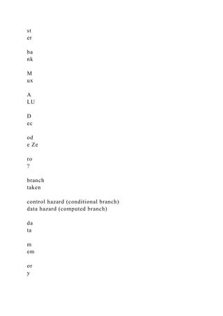
Let (x(t), y(t)) ∈ R2 be the position relative to some fixed
coordinate frame and
θ(t) ∈ (−π, π] be the angle (in radians) of the vehicle at time t,
as shown in
Figure 4.12. In terms of this coordinate frame, the motion of the
vehicle is given
4. HYBRID SYSTEMS
track
AG
V
global
coordinate
frame
Figure 4.12: Illustration of the automated guided vehicle of
Example 4.8. The
vehicle is following a curved painted track, and has deviated
from the track by a
distance e(t). The coordinates of the vehicle at time t with
respect to the global
coordinate frame are (x(t), y(t), θ(t)).
by a system of three differential equations,
ẋ(t) = u(t) cos θ(t),

ẏ(t) = u(t) sin θ(t), (4.6)
θ̇(t) = ω(t).
Equations (4.6) describe the plant. The environment is the
closed painted track. It
could be described by an equation. We will describe it
indirectly below by means
of a sensor.
Figure 4.13: The automatic guided vehicle of Example 4.8 has
four modes: stop,
straight, left, right.
4. HYBRID SYSTEMS
The two-level controller design is based on a simple idea. The
vehicle always
moves at its maximum speed of 10 mph. If the vehicle strays too
far to the left
of the track, the controller steers it towards the right; if it strays
too far to the
right of the track, the controller steers it towards the left. If the
vehicle is close

to the track, the controller maintains the vehicle in a straight
direction. Thus the
controller guides the vehicle in four modes, left, right, straight,
and stop. In stop
mode, the vehicle comes to a halt.
The following differential equations govern the AGV’s motion
in the refinements
of the four modes. They describe the low-level controller, i.e.,
the selection of the
time-based plant inputs in each mode.
straight
ẋ(t) = 10 cos θ(t)
ẏ(t) = 10 sin θ(t)
θ̇(t) = 0
left
ẋ(t) = 10 cos θ(t)
ẏ(t) = 10 sin θ(t)
θ̇(t) = π
right
ẋ(t) = 10 cos θ(t)
ẏ(t) = 10 sin θ(t)
θ̇(t) = −π

stop
ẋ(t) = 0
ẏ(t) = 0
θ̇(t) = 0
In the stop mode, the vehicle is stopped, so x(t), y(t), and θ(t)
are constant. In
the left mode, θ(t) increases at the rate of π radians/second, so
from Figure 4.12
we see that the vehicle moves to the left. In the right mode, it
moves to the right.
In the straight mode, θ(t) is constant, and the vehicle moves
straight ahead with
a constant heading. The refinements of the four modes are
shown in the boxes of
Figure 4.13.
We design the supervisory control governing transitions
between modes in such
a way that the vehicle closely follows the track, using a sensor
that determines
how far the vehicle is to the left or right of the track. We can
build such a sensor
using photodiodes. Let’s suppose the track is painted with a
light-reflecting color,

whereas the floor is relatively dark. Underneath the AGV we
place an array of
photodiodes as shown in Figure 4.14. The array is perpendicular
to the AGV
body axis. As the AGV passes over the track, the diode directly
above the track
generates more current than the other diodes. By comparing the
magnitudes of
the currents through the different diodes, the sensor estimates
the displacement
e(t) of the center of the array (hence, the center of the AGV)
from the track. We
adopt the convention that e(t) < 0 means that the AGV is to the
right of the track
and e(t) > 0 means it is to the left. We model the sensor output
as a function f
of the AGV’s position,
∀ t, e(t) = f(x(t), y(t)).
The function f of course depends on the environment—the track.
We now specify
the supervisory controller precisely. We select two thresholds, 0
< �1 < �2, as
shown in Figure 4.14. If the magnitude of the displacement is
small, |e(t)| < �1,
we consider that the AGV is close enough to the track, and the
AGV can move
straight ahead, in straight mode. If e(t) > �2 (e(t) is large and
positive), the AGV
has strayed too far to the left and must be steered to the right,
by switching to
right mode. If e(t) < −�2 (e(t) is large and negative), the AGV
has strayed too
far to the right and must be steered to the left, by switching to
left mode. This

control logic is captured in the mode transitions of Figure 4.13.
The inputs are
pure signals stop and start. These model an operator that can
stop or start the
AGV. There is no continuous-time input. The outputs represent
the position of
the vehicle, x(t) and y(t). The initial mode is stop, and the
initial values of its
refinement are (x0, y0, θ0).
We analyze how the AGV will move. Figure 4.15 sketches one
possible trajectory.
Initially the vehicle is within distance �1 of the track, so it
moves straight. At some
4. HYBRID SYSTEMS
photodiode trackAGV
Figure 4.14: An array of photodiodes under the AGV is used to
estimate the
displacement e of the AGV relative to the track. The photodiode
directly above
the track generates more current.
later time, the vehicle goes too far to the left, so the guard
¬stop ∧ e(t) > �2
is satisfied, and there is a mode switch to right. After some
time, the vehicle will

again be close enough to the track, so the guard
¬stop ∧ |e(t)| < �1
is satisfied, and there is a mode switch to straight. Some time
later, the vehicle is
too far to the right, so the guard
¬stop ∧ e(t) < −�2
is satisfied, and there is a mode switch to left. And so on.
The example illustrates the four components of a control
system. The plant is described
by the differential equations (4.6) that govern the evolution of
the continuous state at
time t, (x(t), y(t), θ(t)), in terms of the plant inputs u and ω. The
second component
is the environment—the closed track. The third component is
the sensor, whose output
at time t, e(t) = f(x(t), y(t)), gives the position of the AGV
relative to the track. The
fourth component is the two-level controller. The supervisory
controller comprises the
four modes and the guards that determine when to switch
between modes. The low-level
4.3. SUMMARY
initial
position

straight
right
straight
left
track straight
Figure 4.15: A trajectory of the AGV, annotated with modes.
controller specifies how the time-based inputs to the plant, u
and ω, are selected in each
mode.
4.3 Summary
Hybrid systems provide a bridge between time-based models
and state-machine models.
The combination of the two families of models provides a rich
framework for describing
real-world systems. There are two key ideas. First, discrete
events (state changes in a state
machine) get embedded in a time base. Second, a hierarchical
description is particularly
useful, where the system undergoes discrete transitions between
different modes of opera-
tion. Associated with each mode of operation is a time-based
system called the refinement
of the mode. Mode transitions are taken when guards that
specify the combination of in-
puts and continuous states are satisfied. The action associated
with a transition, in turn,
sets the continuous state in the destination mode.

4. HYBRID SYSTEMS
The behavior of a hybrid system is understood using the tools of
state machine analysis
for mode transitions and the tools of time-based analysis for the
refinement systems. The
design of hybrid systems similarly proceeds on two levels: state
machines are designed to
achieve the appropriate logic of mode transitions, and
continuous refinement systems are
designed to secure the desired time-based behavior in each
mode.
EXERCISES
Exercises
1. Construct (on paper is sufficient) a timed automaton similar
to that of Figure 4.7
which produces tick at times 1, 2, 3, 5, 6, 7, 8, 10, 11, · · · .
That is, ticks are produced
with intervals between them of 1 second (three times) and 2
seconds (once).
2. The objective of this problem is to understand a timed

automaton, and then to mod-
ify it as specified.
(a) For the timed automaton shown below, describe the output y.
Avoid imprecise
or sloppy notation.
(b) Assume there is a new pure input reset, and that when this
input is present,
the hybrid system starts over, behaving as if it were starting at
time 0 again.
Modify the hybrid system from part (a) to do this.
3. In Exercise 6 of Chapter 2, we considered a DC motor that is
controlled by an in-
put voltage. Controlling a motor by varying an input voltage, in
reality, is often
not practical. It requires analog circuits that are capable of
handling considerable
power. Instead, it is common to use a fixed voltage, but to turn
it on and off period-
ically to vary the amount of power delivered to the motor. This
technique is called
pulse width modulation (PWM).
Construct a timed automaton that provides the voltage input to
the motor model
from Exercise 6. Your hybrid system should assume that the
PWM circuit delivers
a 25 kHz square wave with a duty cycle between zero and 100%,
inclusive. The
input to your hybrid system should be the duty cycle, and the
output should be the
voltage.

4. HYBRID SYSTEMS
4. Consider the following timed automaton:
Assume that the input signals a and b are discrete continuous-
time signals, meaning
that each can be given as a function of form a : R → {present,
absent}, where at
almost all times t ∈ R, a(t) = absent. Assume that the state
machine can take
at most one transition at each distinct time t, and that machine
begins executing at
time t = 0.
(a) Sketch the output b if the input a is present only at times
t = 0.75, 1.5, 2.25, 3, 3.75, 4.5, · · ·
Include at least times from t = 0 to t = 5.
(b) Sketch the output b if the input a is present only at times t =
0, 1, 2, 3, · · · .
(c) Assuming that the input a can be any discrete signal at all,
find a lower bound
on the amount of time between events b. What input signal a (if
any) achieves
this lower bound?
5. You have an analog source that produces a pure tone. You
can switch the source on
or off by the input event on or off. Construct a timed automaton

that provides the on
and off signals as outputs, to be connected to the inputs of the
tone generator. Your
system should behave as follows. Upon receiving an input event
ring, it should
produce an 80 ms-long sound consisting of three 20 ms-long
bursts of the pure tone
separated by two 10 ms intervals of silence. What does your
system do if it receives
two ring events that are 50 ms apart?
EXERCISES
6. Automobiles today have the features listed below. Implement
each feature as a
timed automaton.
(a) The dome light is turned on as soon as any door is opened. It
stays on for 30
seconds after all doors are shut. What sensors are needed?
(b) Once the engine is started, a beeper is sounded and a red
light warning is
indicated if there are passengers that have not buckled their seat
belt. The
beeper stops sounding after 30 seconds, or as soon the seat belts
are buckled,
whichever is sooner. The warning light is on all the time the
seat belt is un-
buckled. Hint: Assume the sensors provide a warn event when
the ignition

is turned on and there is a seat with passenger not buckled in, or
if the igni-
tion is already on and a passenger sits in a seat without buckling
the seatbelt.
Assume further that the sensors provide a noWarn event when a
passenger de-
parts from a seat, or when the buckle is buckled, or when the
ignition is turned
off.
7. A programmable thermostat allows you to select 4 times, 0 ≤
T1 ≤ · · · ≤ T4 < 24
(for a 24-hour cycle) and the corresponding setpoint
temperatures a1, · · · , a4. Con-
struct a timed automaton that sends the event ai to the heating
systems controller.
The controller maintains the temperature close to the value ai
until it receives the
next event. How many timers and modes do you need?
8. Consider the following timed automaton:
Assume t1 and t2 are positive real numbers. What is the
minimum amount of time
between events a? That is, what is the smallest possible time
between two times
when the signal a is present?
4. HYBRID SYSTEMS
9. Figure 4.16 depicts the intersection of two one-way streets,

called Main and Sec-
ondary. A light on each street controls its traffic. Each light
goes through a cycle
consisting of a red (R), green (G), and yellow (Y) phases. It is a
safety requirement
that when one light is in its green or yellow phase, the other is
in its red phase. The
yellow phase is always 5 seconds long.
The traffic lights operate as follows. A sensor in the secondary
road detects a ve-
hicle. While no vehicle is detected, there is a 4 minute-long
cycle with the main
light having 3 minutes of green, 5 seconds of yellow, and 55
seconds of red. The
secondary light is red for 3 minutes and 5 seconds (while the
main light is green
and yellow), green for 50 seconds, then yellow for 5 seconds.
If a vehicle is detected on the secondary road, the traffic light
quickly gives a right
of way to the secondary road. When this happens, the main light
aborts its green
phase and immediately switches to its 5 second yellow phase. If
the vehicle is
detected while the main light is yellow or red, the system
continues as if there were
no vehicle.
Design a hybrid system that controls the lights. Let this hybrid
system have six
pure outputs, one for each light, named mG, mY, and mR, to
designate the main
Main

S
ec
on
da
ry
light
detector
R
R G
G Y
Y
Figure 4.16: Traffic lights control the intersection of a main
street and a secondary
street. A detector senses when a vehicle crosses it. The red
phase of one light
must coincide with the green and yellow phases of the other
light.
EXERCISES
light being green, yellow, or red, respectively, and sG, sY, and
sR, to designate the

secondary light being green, yellow, or red, respectively. These
signals should be
generated to turn on a light. You can implicitly assume that
when one light is turned
on, whichever has been on is turned off.
10. For the bouncing ball of Example 4.7, let tn be the time
when the ball hits the
ground for the n-th time, and let vn = ẏ(tn) be the velocity at
that time.
(a) Find a relation between vn+1 and vn for n > 1, and then
calculate vn in terms
of v1.
(b) Obtain tn in terms of v1 and a. Use this to show that the
bouncing ball is a
Zeno system. Hint: The geometric series identity might be
useful, where
for |b| < 1,
∞∑
m=0
bm =
1
1− b
.
(c) Calculate the maximum height reached by the ball after
successive bumps.
11. Elaborate the hybrid system model of Figure 4.10 so that in
the together mode, the
stickiness decays according to the differential equation

ṡ(t) = −as(t)
where s(t) is the stickiness at time t, and a is some positive
constant. On the tran-
sition into this mode, the stickiness should be initialized to
some starting stickiness
b.
12. Show that the trajectory of the AGV of Figure 4.13 while it
is in left or right mode
is a circle. What is the radius of this circle, and how long does
it take to complete a
circle?
13. Consider Figure 4.17 depicting a system comprising two
tanks containing water.
Each tank is leaking at a constant rate. Water is added at a
constant rate to the
system through a hose, which at any point in time is filling
either one tank or the
other. It is assumed that the hose can switch between the tanks
instantaneously.
For i ∈ {1, 2}, let xi denote the volume of water in Tank i and
vi > 0 denote the
constant flow of water out of Tank i. Letw denote the constant
flow of water into the
system. The objective is to keep the water volumes above r1 and
r2, respectively,
assuming that the water volumes are above r1 and r2 initially.
This is to be achieved

4. HYBRID SYSTEMS
x1
r1
v1
x2
r2
v2
w
Figure 4.17: Water tank system.
by a controller that switches the inflow to Tank 1 whenever
x1(t) ≤ r1(t) and to
Tank 2 whenever x2(t) ≤ r2(t).
The hybrid automaton representing this two-tank system is
given in Figure 4.18.
Answer the following questions:
(a) Construct a model of this hybrid automaton in Ptolemy II,
LabVIEW, or
Simulink. Use the following parameter values: r1 = r2 = 0, v1 =
v2 = 0.5,
and w = 0.75. Set the initial state to be (q1, (0, 1)). (That is,
initial value
x1(0) is 0 and x2(0) is 1.)
Verify that this hybrid automaton is Zeno. What is the reason
for this Zeno

behavior? Simulate your model and plot how x1 and x2 vary as
a function of
time t, simulating long enough to illustrate the Zeno behavior.
(b) A Zeno system may be regularized by ensuring that the time
between tran-
sitions is never less than some positive number �. This can be
emulated by
inserting extra modes in which the hybrid automaton dwells for
time �. Use
regularization to make your model from part (a) non-Zeno.
Again, plot x1
and x2 for the same length of time as in the first part. State the
value of � that
you used.
Include printouts of your plots with your answer.
EXERCISES
Figure 4.18: Hybrid automaton representing water tank system.
5
Composition of
State Machines

5.1 Concurrent Composition . . . . . . . . . . . . . . . . . . . . . . . 111
Sidebar: About Synchrony . . . . . . . . . . . . . . . . . . . . . . . 112
5.1.1 Side-by-Side Synchronous Composition . . . . . . . . . . . .
113
5.1.2 Side-by-Side Asynchronous Composition . . . . . . . . . . .
116
Sidebar: Scheduling Semantics for Asynchronous Composition .
. . . 118
5.1.3 Shared Variables . . . . . . . . . . . . . . . . . . . . . . . . 119
5.1.4 Cascade Composition . . . . . . . . . . . . . . . . . . . . . 122
5.1.5 General Composition . . . . . . . . . . . . . . . . . . . . . . 125
5.2 Hierarchical State Machines . . . . . . . . . . . . . . . . . . . . .
126
5.3 Summary . . . . . . . . . . . . . . . . . . . . . . . . . . . . . . . . 130
Exercises . . . . . . . . . . . . . . . . . . . . . . . . . . . . . . . . . . . 132
State machines provide a convenient way to model behaviors of
systems. One disadvan-
tage that they have is that for most interesting systems, the
number of states is very large,
often even infinite. Automated tools can handle large state
spaces, but humans have more
difficulty with any direct representation of a large state space.
A time-honored principle in engineering is that complicated
systems should be described
as compositions of simpler systems. This chapter gives a
number of ways to do this with
state machines. The reader should be aware, however, that there
are many subtly different
ways to compose state machines. Compositions that look similar
on the surface may mean

different things to different people. The rules of notation of a
model are called its syntax,
and the meaning of the notation is called its semantics.
Example 5.1: In the standard syntax of arithmetic, a plus sign +
has a number or
expression before it, and a number or expression after it. Hence,
1+2, a sequence
of three symbols, is a valid arithmetic expression, but 1+ is not.
The semantics of
the expression 1 + 2 is the addition of two numbers. This
expression means “the
number three, obtained by adding 1 and 2.” The expression 2 +
1 is syntactically
different, but semantically identical (because addition is
commutative).
The models in this book predominantly use a visual syntax,
where the elements are boxes,
circles, arrows, etc., rather than characters in a character set,
and where the positioning
of the elements is not constrained to be a sequence. Such
syntaxes are less standardized
than, for example, the syntax of arithmetic. We will see that the
same syntax can have
many different semantics, which can cause no end of confusion.
Example 5.2: A now popular notation for concurrent
composition of state
machines called Statecharts was introduced by Harel (1987).
Although they
are all based on the same original paper, many variants of
Statecharts have
evolved (von der Beeck, 1994). These variants often assign
different semantics to
the same syntax.

In this chapter, we assume an actor model for extended state
machines using the syntax
summarized in Figure 5.1. The semantics of a single such state
machine is described in
Chapter 3. This chapter will discuss the semantics that can be
assigned to compositions
of multiple such machines.
The first composition technique we consider is concurrent
composition. Two or more
state machines react either simultaneously or independently. If
the reactions are simul-
taneous, we call it synchronous composition. If they are
independent, then we call it
5. COMPOSITION OF STATE MACHINES
asynchronous composition. But even within these classes of
composition, many subtle
variations in the semantics are possible. These variations mostly
revolve around whether
and how the state machines communicate and share variables.
The second composition technique we will consider is
hierarchy. Hierarchical state ma-
chines can also enable complicated systems to be described as
compositions of simpler
systems. Again, we will see that subtle differences in semantics
are possible.

5.1 Concurrent Composition
To study concurrent composition of state machines, we will
proceed through a sequence
of patterns of composition. These patterns can be combined to
build arbitrarily compli-
cated systems. We begin with the simplest case, side-by-side
composition, where the
state machines being composed do not communicate. We then
consider allowing com-
munication through shared variables, showing that this creates
significant subtleties that
can complicate modeling. We then consider communication
through ports, first looking
at serial composition, then expanding to arbitrary
interconnections. We consider both
synchronous and asynchronous composition for each type of
composition.
i1
in om
o1
... ...
Figure 5.1: Summary of notation for state machines used in this
chapter.
5.1. CONCURRENT COMPOSITION

About Synchrony
The term synchronous means (1) occurring or existing at the
same time or (2) moving
or operating at the same rate. In engineering and computer
science, the term has a num-
ber of meanings that are mostly consistent with these
definitions, but oddly inconsistent
with one another. In referring to concurrent software
constructed using threads or pro-
cesses, synchronous communication refers to a rendezvous style
of communication,
where the sender of a message must wait for the receiver to be
ready to receive, and
the receiver must wait for the sender. Conceptually, the two
threads see the communi-
cation occurring at the same time, consistent with definition (1).
In Java, the keyword
synchronized defines blocks of code that are not permitted to
execute simultane-
ously. Oddly, two code blocks that are synchronized cannot
“occur” (execute) at the
same time, which is inconsistent with both definitions.
In the world of software, there is yet a third meaning of the
word synchronous, and
it is this third meaning that we use in this chapter. This third
meaning underlies the
synchronous languages (see box on page 148). Two key ideas
govern these languages.
First, the outputs of components in a program are (conceptually)
simultaneous with
their inputs (this is called the synchrony hypothesis). Second,
components in a pro-
gram execute (conceptually) simultaneously and
instantaneously. Real executions do
not literally occur simultaneously nor instantaneously, and

outputs are not really si-
multaneous with the inputs, but a correct execution must behave
as if they were. This
use of the word synchronous is consistent with both definitions
above; executions of
components occur at the same time and operate at the same rate.
In circuit design, the word synchronous refers to a style of
design where a clock that
is distributed throughout a circuit drives latches that record
their inputs on edges of the
clock. The time between clock edges needs to be sufficient for
circuits between latches
to settle. Conceptually, this model is similar to the model in
synchronous languages.
Assuming that the circuits between latches have zero delay is
equivalent to the syn-
chrony hypothesis, and global clock distribution gives
simultaneous and instantaneous
execution.
In power systems engineering, synchronous means that
electrical waveforms have
the same frequency and phase. In signal processing,
synchronous means that signals
have the same sample rate, or that their sample rates are fixed
multiples of one an-
other. The term synchronous dataflow, described in Section
6.3.2, is based on this
latter meaning of the word synchronous. This usage is
consistent with definition (2).

5.1.1 Side-by-Side Synchronous Composition
The first pattern of composition that we consider is side-by-side
composition, illustrated
for two actors in Figure 5.2. In this pattern, we assume that the
inputs and outputs of the
two actors are disjoint, i.e., that the state machines do not
communicate. In the figure, ac-
tor A has input i1 and output o1, and actor B has input i2 and
output o2. The composition
of the two actors is itself an actor C with inputs i1 and i2 and
outputs o1 and o2.1
In the simplest scenario, if the two actors are extended state
machines with variables,
then those variables are also disjoint. We will later consider
what happens when the two
state machines share variables. Under synchronous composition,
a reaction of C is a
simultaneous reaction of A and B.
Example 5.3: Consider FSMsA andB in Figure 5.3. A has a
single pure output
a, andB has a single pure output b. The side-by-side
composition C has two pure
outputs, a and b. If the composition is synchronous, then on the
first reaction, a
will be absent and b will be present. On the second reaction, it
will be the reverse.
On subsequent reactions, a and b will continue to alternate
being present.
1The composition actor C may rename these input and output

ports, but here we assume it uses the same
names as the component actors.
Figure 5.2: Side-by-side composition of two actors.
Figure 5.3: Example of side-by-side composition of two actors.
Synchronous side-by-side composition is simple for several
reasons. First, recall from
Section 3.3.2 that the environment determines when a state
machine reacts. In syn-
chronous side-by-side composition, the environment need not be
aware that C is a com-
position of two state machines. Such compositions are modular
in the sense that the
composition itself becomes a component that can be further
composed as if it were itself
an atomic component.
Moreover, if the two state machines A and B are deterministic,
then the synchronous
side-by-side composition is also deterministic. We say that a
property is compositional if
a property held by the components is also a property of the
composition. For synchronous
side-by-side composition, determinism is a compositional
property.
In addition, a synchronous side-by-side composition of finite

state machines is itself an
FSM. A rigorous way to give the semantics of the composition
is to define a single state
machine for the composition. Suppose that as in Section 3.3.3,
state machines A and B
are given by the five tuples,
A = (StatesA, InputsA,OutputsA, updateA, initialStateA)
B = (StatesB, InputsB,OutputsB, updateB, initialStateB) .
Then the synchronous side-by-side composition C is given by
StatesC = StatesA × StatesB (5.1)
InputsC = InputsA × InputsB (5.2)
OutputsC = OutputsA × OutputsB (5.3)
initialStateC = (initialStateA, initialStateB) (5.4)
and the update function is defined by
updateC((sA, sB), (iA, iB)) = ((s
′
A, s
′
B), (oA, oB)),
where

(s′A, oA) = updateA(sA, iA),
and
(s′B, oB) = updateB(sB, iB),
for all sA ∈ StatesA, sB ∈ StatesB , iA ∈ InputsA, and iB ∈
InputsB .
Recall that InputsA and InputsB are sets of valuations. Each
valuation in the set is an
assignment of values to ports. What we mean by
InputsC = InputsA × InputsB
is that a valuation of the inputs of C must include both
valuations for the inputs of A and
the inputs of B.
As usual, the single FSMC can be given pictorially rather than
symbolically, as illustrated
in the next example.
Example 5.4: The synchronous side-by-side composition C in
Figure 5.3 is
given as a single FSM in Figure 5.4. Notice that this machine
behaves exactly as
described in Example 5.3. The outputs a and b alternate being
present. Notice
further that (s1, s4) and (s2, s3) are not reachable states.

Figure 5.4: Single state machine giving the semantics of
synchronous side-by-
side composition of the state machines in Figure 5.3.
5.1.2 Side-by-Side Asynchronous Composition
In an asynchronous composition of state machines, the
component machines react inde-
pendently. This statement is rather vague, and in fact, it has
several different interpreta-
tions. Each interpretation gives a semantics to the composition.
The key to each semantics
is how to define a reaction of the composition C in Figure 5.2.
Two possibilities are:
• Semantics 1. A reaction of C is a reaction of one of A or B,
where the choice is
nondeterministic.
• Semantics 2. A reaction of C is a reaction of A, B, or both A
and B, where the
choice is nondeterministic. A variant of this possibility might
allow neither to react.
Semantics 1 is referred to as an interleaving semantics, meaning
that A or B never react
simultaneously. Their reactions are interleaved in some order.
A significant subtlety is that under these semantics machines A
and B may completely
miss input events. That is, an input to C destined for machine A
may be present in a
reaction where the nondeterministic choice results in B reacting
rather than A. If this is
not desirable, then some control over scheduling (see sidebar on

) or synchronous
composition becomes a better choice.
Figure 5.5: State machine giving the semantics of asynchronous
side-by-side
composition of the state machines in Figure 5.3.
Example 5.5: For the example in Figure 5.3, semantics 1 results
in the composi-
tion state machine shown in Figure 5.5. This machine is
nondeterministic. From
state (s1, s3), when C reacts, it can move to (s2, s3) and emit no
output, or it
can move to (s1, s4) and emit b. Note that if we had chosen
semantics 2, then it
would also be able to move to (s2, s4).
For asynchronous composition under semantics 1, the symbolic
definition of C has the
same definitions of StatesC , InputsC , OutputsC , and
initialStateC as for synchronous
composition, given in (5.1) through (5.4). But the update
function differs, becoming
updateC((sA, sB), (iA, iB)) = ((s
′
A, s
′
B), (o

′
A, o
′
B)),
where either
(s′A, o
′
A) = updateA(sA, iA) and s
′
B = sB and o
′
B = absent
or
(s′B, o
′
B) = updateB(sB, iB) and s
′
A = sA and o
′
A = absent

for all sA ∈ StatesA, sB ∈ StatesB , iA ∈ InputsA, and iB ∈
InputsB . What we mean by
o′B = absent is that all outputs of B are absent. Semantics 2 can
be similarly defined (see
Exercise 2).
Scheduling Semantics for Asynchronous Composition
In the case of semantics 1 and 2 given in Section 5.1.2, the
choice of which compo-
nent machine reacts is nondeterministic. The model does not
express any particular
constraints. It is often more useful to introduce some scheduling
policies, where the
environment is able to influence or control the nondeterministic
choice. This leads to
two additional possible semantics for asynchronous
composition:
• Semantics 3. A reaction of C is a reaction of one of A or B,
where the environ-
ment chooses which of A or B reacts.
• Semantics 4. A reaction of C is a reaction of A, B, or both A
and B, where the
choice is made by the environment.
Like semantics 1, semantics 3 is an interleaving semantics.
In one sense, semantics 1 and 2 are more compositional than
semantics 3 and 4.
To implement semantics 3 and 4, a composition has to provide
some mechanism for
the environment to choose which component machine should

react (for scheduling the
component machines). This means that the hierarchy suggested
in Figure 5.2 does not
quite work. Actor C has to expose more of its internal structure
than just the ports and
the ability to react.
In another sense, semantics 1 and 2 are less compositional than
semantics 3 and 4
because determinism is not preserved by composition. A
composition of deterministic
state machines is not a deterministic state machine.
Notice further that semantics 1 is an abstraction of semantics 3
in the sense that
every behavior under semantics 3 is also a behavior under
semantics 1. This notion of
abstraction is studied in detail in Chapter 14.
The subtle differences between these choices make
asynchronous composition
rather treacherous. Considerable care is required to ensure that
it is clear which
semantics is used.
Figure 5.6: Model of two servers with a shared task queue,
assuming asyn-
chronous composition under semantics 1.

5.1.3 Shared Variables
An extended state machine has local variables that can be read
and written as part of
taking a transition. Sometimes it is useful when composing state
machines to allow these
variables to be shared among a group of machines. In particular,
such shared variables can
be useful for modeling interrupts, studied in Chapter 10, and
threads, studied in Chapter
11. However, considerable care is required to ensure that the
semantics of the model
conforms with that of the program containing interrupts or
threads. Many complications
arise, including the memory consistency model and the notion
of atomic operations.
Example 5.6: Consider two servers that can receive requests
from a network.
Each request requires an unknown amount of time to service, so
the servers share
a queue of requests. If one server is busy, the other server can
respond to a request,
even if the request arrives at the network interface of the first
server.
This scenario fits a pattern similar to that in Figure 5.2, where
A and B are the
servers. We can model the servers as state machines as shown in

Figure 5.6. In
this model, a shared variable pending counts the number of
pending job requests.
When a request arrives at the composite machine C, one of the
two servers is
nondeterministically chosen to react, assuming asynchronous
composition under
semantics 1. If that server is idle, then it proceeds to serve the
request. If the
server is serving another request, then one of two things can
happen: it can co-
incidentally finish serving the request it is currently serving,
issuing the output
done, and proceed to serve the new one, or it can increment the
count of pending
requests and continue to serve the current request. The choice
between these is
nondeterministic, to model the fact that the time it takes to
service a request is
unknown.
If C reacts when there is no request, then again either server A
or B will be se-
lected nondeterministically to react. If the server that reacts is
idle and there are
one or more pending requests, then the server transitions to
serving and decre-
ments the variable pending. If the server that reacts is not idle,
then one of three
things can happen. It may continue serving the current request,
in which case it
simply transitions on the self transition back to serving. Or it
may finish serving
the request, in which case it will transition to idle if there are
no pending requests,
or transition back to serving and decrement pending if there are

pending requests.
The model in the previous example exhibits many subtleties of
concurrent systems. First,
because of the interleaving semantics, accesses to the shared
variable are atomic opera-
tions, something that is quite challenging to guarantee in
practice, as discussed in Chapters
10 and 11. Second, the choice of semantics 1 is reasonable in
this case because the input
goes to both of the component machines, so regardless of which
component machine re-
acts, no input event will be missed. However, this semantics
would not work if the two
machines had independent inputs, because then requests could
be missed. Semantics 2
can help prevent that, but what strategy should be used by the
environment to determine
which machine reacts? What if the two independent inputs both
have requests present at
the same reaction ofC? If we choose semantics 4 in the sidebar
on page 118 to allow both
machines to react simultaneously, then what is the meaning
when both machines update
the shared variable? The updates are no longer atomic, as they
are with an interleaving
semantics.

Note further that choosing asynchronous composition under
semantics 1 allows behaviors
that do not make good use of idle machines. In particular,
suppose that machine A is
serving, machine B is idle, and a request arrives. If the
nondeterministic choice results in
machineA reacting, then it will simply increment pending. Not
until the nondeterministic
choice results inB reacting will the idle machine be put to use.
In fact, semantics 1 allows
behaviors that never use one of the machines.
Shared variables may be used in synchronous compositions as
well, but sophisticated
subtleties again emerge. In particular, what should happen if in
the same reaction one ma-
chine reads a shared variable to evaluate a guard and another
machine writes to the shared
variable? Do we require the write before the read? What if the
transition doing the write
to the shared variable also reads the same variable in its guard
expression? One possibil-
ity is to choose a synchronous interleaving semantics, where the
component machines
react in arbitrary order, chosen nondeterministically. This
strategy has the disadvantage
that a composition of two deterministic machines may be
nondeterministic. An alterna-
tive version of the synchronous interleaving semantics has the
component machines react
in a fixed order determined by the environment or by some
additional mechanism such as
priority.
The difficulties of shared variables, particularly with
asynchronous composition, reflect

the inherent complexity of concurrency models with shared
variables. Clean solutions
require a more sophisticated semantics, to be discussed in
Chapter 6. In that chapter, we
will explain the synchronous-reactive model of computation,
which gives a synchronous
composition semantics that is reasonably compositional.
So far, we have considered composition of machines that do not
directly communicate.
We next consider what happens when the outputs of one
machine are the inputs of another.
5.1.4 Cascade Composition
Consider two state machines A and B that are composed as
shown in Figure 5.7. The
output of machine A feeds the input of B. This style of
composition is called cascade
composition or serial composition.
In the figure, output port o1 from A feeds events to input port i2
of B. Assume the data
type of o1 is V1 (meaning that o1 can take values from V1 or be
absent), and the data type
of i2 is V2. Then a requirement for this composition to be valid
is that
V1 ⊆ V2 .

This asserts that any output produced by A on port o1 is an
acceptable input to B on port
i2. The composition type checks.
For cascade composition, if we wish the composition to be
asynchronous, then we need
to introduce some machinery for buffering the data that is sent
from A to B. We defer
discussion of such asynchronous composition to Chapter 6,
where dataflow and process
network models of computation will provide such asynchronous
composition. In this
chapter, we will only consider synchronous composition for
cascade systems.
In synchronous composition of the cascade structure of Figure
5.7, a reaction ofC consists
of a reaction of both A and B, where A reacts first, produces its
output (if any), and then
B reacts. Logically, we view this as occurring in zero time, so
the two reactions are in a
sense simultaneous and instantaneous. But they are causally
related in that the outputs
of A can affect the behavior of B.
Figure 5.7: Cascade composition of two actors.
Figure 5.8: Example of a cascade composition of two FSMs.

Figure 5.9: Semantics of the cascade composition of Figure 5.8,
assuming syn-
chronous composition.
Example 5.7: Consider the cascade composition of the two
FSMs in Figure
5.8. Assuming synchronous semantics, the meaning of a
reaction of C is given in
Figure 5.9. That figure makes it clear that the reactions of the
two machines are
simultaneous and instantaneous. When moving from the initial
state (s1, s3) to
(s2, s4) (which occurs when the input a is absent), the
composition machine C
does not pass through (s2, s3)! In fact, (s2, s3) is not a
reachable state! In this
way, a single reaction of C encompasses a reaction of both A
and B.
To construct the composition machine as in Figure 5.9, first
form the state space as the
cross product of the state spaces of the component machines,
and then determine which
transitions are taken under what conditions. It is important to
remember that the transi-
tions are simultaneous, even when one logically causes the
other.

Example 5.8: Recall the traffic light model of Figure 3.10.
Suppose that we
wish to compose this with a model of a pedestrian crossing
light, like that shown
in Figure 5.10. The output sigR of the traffic light can provide
the input sigR
of the pedestrian light. Under synchronous cascade composition,
the meaning of
the composite is given in Figure 5.11. Note that unsafe states,
such as (green,
green), which is the state when both cars and pedestrians have a
green light, are
not reachable states, and hence are not shown.
In its simplest form, cascade composition implies an ordering of
the reactions of the
Figure 5.10: A model of a pedestrian crossing light, to be
composed in a syn-
chronous cascade composition with the traffic light model of
Figure 3.10.
Figure 5.11: Semantics of a synchronous cascade composition
of the traffic light
model of Figure 3.10 with the pedestrian light model of Figure
5.10.
components. Since this ordering is well defined, we do not have

as much difficulty with
shared variables as we did with side-by-side composition.
However, we will see that in
more general compositions, the ordering is not so simple.
5.1.5 General Composition
Side-by-side and cascade composition provide the basic
building blocks for building more
complex compositions of machines. Consider for example the
composition in Figure 5.12.
A1 and A3 are a side-by-side composition that together define a
machine B. B and A2
are a cascade composition, with B feeding events to A2.
However, B and A2 are also
a cascade composition in the opposite order, with A2 feeding
events to B. Cycles like
5.2. HIERARCHICAL STATE MACHINES
Figure 5.12: Arbitrary interconnections of state machines are
combinations of
side-by-side and cascade compositions, possibly creating
cycles, as in this ex-
ample.
this are called feedback, and they introduce a conundrum; which
machine should react
first, B or A2? This conundrum will be resolved in the next
chapter when we explain the
synchronous-reactive model of computation.

5.2 Hierarchical State Machines
In this section, we consider hierarchical FSMs, which date back
to Statecharts (Harel,
1987). There are many variants of Statecharts, often with subtle
semantic differences
between them (von der Beeck, 1994). Here, we will focus on
some of the simpler aspects
only, and we will pick a particular semantic variant.
The key idea in hierarchical state machines is state refinement.
In Figure 5.13, state B has
a refinement that is another FSM with two states, C and D.
What it means for the machine
to be in state B is that it is in one of states C or D.
The meaning of the hierarchy in Figure 5.13 can be understood
by comparing it to the
equivalent flattened FSM in Figure 5.14. The machine starts in
state A. When guard g2
evaluates to true, the machine transitions to state B, which
means a transition to state C,
the initial state of the refinement. Upon taking this transition to
C, the machine performs
action a2, which may produce an output event or set a variable
(if this is an extended state
machine).
There are then two ways to exit C. Either guard g1 evaluates to
true, in which case the
machine exits B and returns to A, or guard g4 evaluates to true
and the machine transitions
to D. A subtle question is what happens if both guards g1 and
g4 evaluate to true. Different

Figure 5.13: In a hierarchical FSM, a state may have a
refinement that is another
state machine.
Figure 5.14: Semantics of the hierarchical FSM in Figure 5.13.
variants of Statecharts may make different choices at this point.
It seems reasonable that
the machine should end up in state A, but which of the actions
should be performed, a4,
a1, or both? Such subtle questions help account for the
proliferation of different variants
of Statecharts.
We choose a particular semantics that has attractive modularity
properties (Lee and Tri-
pakis, 2010). In this semantics, a reaction of a hierarchical FSM
is defined in a depth-first
fashion. The deepest refinement of the current state reacts first,
then its container state
machine, then its container, etc. In Figure 5.13, this means that
if the machine is in state
5.2. HIERARCHICAL STATE MACHINES

Figure 5.15: Variant of Figure 5.13 that uses a preemptive
transition.
Figure 5.16: Semantics of Figure 5.15 with a preemptive
transition.
B (which means that it is in either C or D), then the refinement
machine reacts first. If
it is C, and guard g4 is true, the transition is taken to D and
action a4 is performed. But
then, as part of the same reaction, the top-level FSM reacts. If
guard g1 is also true, then
the machine transitions to state A. It is important that logically
these two transitions are
simultaneous and instantaneous, so the machine does not
actually go to state D. Nonethe-
less, action a4 is performed, and so is action a1. This
combination corresponds to the
topmost transition of Figure 5.14.
Another subtlety is that if two (non-absent) actions are
performed in the same reaction,
they may conflict. For example, two actions may write different
values to the same output
port. Or they may set the same variable to different values. Our
choice is that the actions
are performed in sequence, as suggested by the semicolon in the
action a4; a1. As in an
imperative language like C, the semicolon denotes a sequence.
If the two actions conflict,
the later one dominates.

Figure 5.17: Variant of the hierarchical state machine of Figure
5.13 that has a
history transition.
Such subtleties can be avoided by using a preemptive transition,
shown in Figure 5.15,
which has the semantics shown in Figure 5.16. The guards of a
preemptive transition are
evaluated before the refinement reacts, and if any guard
evaluates to true, the refinement
does not react. As a consequence, if the machine is in state B
and g1 is true, then neither
action a3 nor a4 is performed. A preemptive transition is shown
with a (red) circle at the
originating end of the transition.
Notice in Figures 5.13 and 5.14 that whenever the machine
enters B, it always enters C,
never D, even if it was previously in D when leaving B. The
transition from A to B is called
a reset transition because the destination refinement is reset to
its initial state, regardless
of where it had previously been. A reset transition is indicated
in our notation with a
hollow arrowhead at the destination end of a transition.
In Figure 5.17, the transition from A to B is a history transition,
an alternative to a reset
transition. In our notation, a solid arrowhead denotes a history
transition. It may also
be marked with an “H” for emphasis. When a history transition
is taken, the destination

refinement resumes in whatever state it was last in (or its initial
state on the first entry).
The semantics of the history transition is shown in Figure 5.18.
The initial state is labeled
(A, C) to indicate that the machine is in state A, and if and
when it next enters B it will go
5.3. SUMMARY
Figure 5.18: Semantics of the hierarchical state machine of
Figure 5.17 that has
a history transition.
to C. The first time it goes to B, it will be in the state labeled
(B, C) to indicate that it is
in state B and, more specifically, C. If it then transitions to (B,
D), and then back to A, it
will end up in the state labeled (A, D), which means it is in
state A, but if and when it next
enters B it will go to D. That is, it remembers its history,
specifically where it was when it
left B.
As with concurrent composition, hierarchical state machines
admit many possible mean-
ings. The differences can be subtle. Considerable care is
required to ensure that models
are clear and that their semantics match what is being modeled.
5.3 Summary

Any well-engineered system is a composition of simpler
components. In this chapter, we
have considered two forms of composition of state machines,
concurrent composition and
hierarchical composition.
For concurrent composition, we introduced both synchronous
and asynchronous compo-
sition, but did not complete the story. We have deferred dealing
with feedback to the
next chapter, because for synchronous composition, significant
subtleties arise. For asyn-
chronous composition, communication via ports requires
additional mechanisms that are
not (yet) part of our model of state machines. Even without
communication via ports,
significant subtleties arise because there are several possible
semantics for asynchronous
composition, and each has strengths and weaknesses. One
choice of semantics may be
suitable for one application and not for another. These
subtleties motivate the topic of the
next chapter, which provides more structure to concurrent
composition and resolves most
of these questions (in a variety of ways).
For hierarchical composition, we focus on a style originally

introduced by Harel (1987)
known as Statecharts. We specifically focus on the ability for
states in an FSM to have
refinements that are themselves state machines. The reactions of
the refinement FSMs are
composed with those of the machine that contains the
refinements. As usual, there are
many possible semantics.
EXERCISES
Exercises
1. Consider the extended state machine model of Figure 3.8, the
garage counter. Sup-
pose that the garage has two distinct entrance and exit points.
Construct a side-by-
side concurrent composition of two counters that share a
variable c that keeps track
of the number of cars in the garage. Specify whether you are
using synchronous or
asynchronous composition, and define exactly the semantics of
your composition
by giving a single machine modeling the composition. If you
choose synchronous
semantics, explain what happens if the two machines
simultaneously modify the
shared variable. If you choose asynchronous composition,
explain precisely which
variant of asynchronous semantics you have chosen and why. Is
your composition

machine deterministic?
2. For semantics 2 in Section 5.1.2, give the five tuple for a
single machine represent-
ing the composition C,
(StatesC , InputsC ,OutputsC , updateC , initialStateC)
for the side-by-side asynchronous composition of two state
machines A and B.
Your answer should be in terms of the five-tuple definitions for
A and B,
(StatesA, InputsA,OutputsA, updateA, initialStateA)
and
(StatesB, InputsB,OutputsB, updateB, initialStateB)
3. Consider the following synchronous composition of two state
machines A and B:
Construct a single state machine C representing the
composition. Which states of
the composition are unreachable?
4. Consider the following synchronous composition of two state
machines A and B:
Construct a single state machine C representing the

composition. Which states of
the composition are unreachable?
5. Consider the following hierarchical state machine:
Construct an equivalent flat FSM giving the semantics of the
hierarchy. Describe
in words the input/output behavior of this machine. Is there a
simpler machine
that exhibits the same behavior? (Note that equivalence
relations between state
machines are considered in Chapter 14, but here, you can use
intuition and just
consider what the state machine does when it reacts.)
6. How many reachable states does the following state machine
have?
EXERCISES
7. Suppose that the machine of Exercise 8 of Chapter 4 is
composed in a synchronous
side-by-side composition with the following machine:
Find a tight lower bound on the time between events a and b.
That is, find a lower
bound on the time gap during which there are no events in
signals a or b. Give an
argument that your lower bound is tight.

6
Concurrent
Models of Computation
6.1 Structure of Models . . . . . . . . . . . . . . . . . . . . . . . . . . 137
Sidebar: Actor Networks as a System of Equations . . . . . . . . . .
139
Sidebar: Fixed-Point Semantics . . . . . . . . . . . . . . . . . . . . 140
6.2 Synchronous-Reactive Models . . . . . . . . . . . . . . . . . . . .
141
6.2.1 Feedback Models . . . . . . . . . . . . . . . . . . . . . . . . 141
6.2.2 Well-Formed and Ill-Formed Models . . . . . . . . . . . . . 143
6.2.3 Constructing a Fixed Point . . . . . . . . . . . . . . . . . . . 145
6.3 Dataflow Models of Computation . . . . . . . . . . . . . . . . . . .
147
Sidebar: Synchronous-Reactive Languages . . . . . . . . . . . . . .
148
6.3.1 Dataflow Principles . . . . . . . . . . . . . . . . . . . . . . . 149
6.3.2 Synchronous Dataflow . . . . . . . . . . . . . . . . . . . . . 152
6.3.3 Dynamic Dataflow . . . . . . . . . . . . . . . . . . . . . . . 157
6.3.4 Structured Dataflow . . . . . . . . . . . . . . . . . . . . . . 158
6.3.5 Process Networks . . . . . . . . . . . . . . . . . . . . . . . . 159
6.4 Timed Models of Computation . . . . . . . . . . . . . . . . . . . .
162
6.4.1 Time-Triggered Models . . . . . . . . . . . . . . . . . . . . 162
6.4.2 Discrete Event Systems . . . . . . . . . . . . . . . . . . . . . 163
6.4.3 Continuous-Time Systems . . . . . . . . . . . . . . . . . . . 164

6.5 Summary . . . . . . . . . . . . . . . . . . . . . . . . . . . . . . . . 167
Sidebar: Petri Nets . . . . . . . . . . . . . . . . . . . . . . . . . . . 168
Sidebar: Models of Time . . . . . . . . . . . . . . . . . . . . . . . . 169
Sidebar: Probing Further: Discrete Event Semantics . . . . . . . . .
170
Exercises . . . . . . . . . . . . . . . . . . . . . . . . . . . . . . . . . . . 172
In sound engineering practice, systems are built by composing
components. In order for
the composition to be well understood, we need first for the
individual components to be
well understood, and then for the meaning of the interaction
between components to be
well understood. The previous chapter dealt with composition of
finite state machines.
With such composition, the components are well defined (they
are FSMs), but there are
many possible interpretations for the interaction between
components. The meaning of a
composition is referred to as its semantics.
This chapter focuses on the semantics of concurrent
composition. The word “concurrent”
literally means “running together.” A system is said to be
concurrent if different parts of
the system (components) conceptually operate at the same time.
There is no particular
order to their operations. The semantics of such concurrent
operation can be quite subtle,
however.
The components we consider in this chapter are actors, which
react to stimuli at input

ports and produce stimuli on output ports. In this chapter, we
will be only minimally
concerned with how the actors themselves are defined. They
may be FSMs, hardware,
or programs specified in an imperative programming language.
We will need to impose
some constraints on what these actors can do, but we need not
constrain how they are
specified.
The semantics of a concurrent composition of actors is governed
by three sets of rules that
we collectively call a model of computation (MoC). The first set
of rules specifies what
constitutes a component. The second set specifies the
concurrency mechanisms. The third
specifies the communication mechanisms.
In this chapter, a component will be an actor with ports and a
set of execution actions.
An execution action defines how the actor reacts to inputs to
produce outputs and change
state. The ports will be interconnected to provide for
communication between actors,
and the execution actions will be invoked by the environment of
the actor to cause the
actor to perform its function. For example, for FSMs, one action
is provided that causes
a reaction. The focus of this chapter is on introducing a few of
the possible concurrency
and communication mechanisms that can govern the interactions
between such actors.
We begin by laying out the common structure of models that
applies to all MoCs studied
in this chapter. We then proceed to describe a suite of MoCs.

6. CONCURRENT MODELS OF COMPUTATION
Figure 6.1: Any interconnection of actors can be modeled as a
single (side-by-
side composite) actor with feedback.
6.1 Structure of Models
In this chapter, we assume that models consist of fixed
interconnections of actors like
that shown in Figure 6.1(a). The interconnections between
actors specify communication
paths. The communication itself takes the form of a signal,
which consists of one or more
communication events. For the discrete signals of Section 3.1,
for example, a signal s
has the form of a function
s : R→ Vs ∪ {absent},
where Vs is a set of values called the type of the signal s. A
communication event in this
case is a non-absent value of s.
6.1. STRUCTURE OF MODELS

Example 6.1: Consider a pure signal s that is a discrete signal
given by
s(t) =
{
present if t is a multiple of P
absent otherwise
for all t ∈ R and some P ∈ R. Such a signal is called a clock
signal with period
P . Communication events occur every P time units.
In Chapter 2, a continuous-time signal has the form of a
function
s : R→ Vs,
in which case every one of the (uncountably) infinite set of
values s(t), for all t ∈ R, is a
communication event. In this chapter, we will also encounter
signals of the form
s : N→ Vs,
where there is no time line. The signal is simply a sequence of
values.
A communication event has a type, and we require that a
connection between actors type
check. That is, if an output port y with type Vy is connected to
an input port x with type
Vx, then
Vy ⊆ Vx.

As suggested in Figure 6.1(b-d), any actor network can be
reduced to a rather simple
form. If we rearrange the actors as shown in Figure 6.1(b), then
the actors form a side-by-
side composition indicated by the box with rounded corners.
This box is itself an actor
F as shown in Figure 6.1(c) whose input is a three-tuple (s1, s2,
s3) of signals and whose
output is the same three-tuple of signals. If we let s = (s1, s2,
s3), then the actor can be
depicted as in Figure 6.1(d), which hides all the complexity of
the model.
Notice that Figure 6.1(d) is a feedback system. By following the
procedure that we used
to build it, every interconnection of actors can be structured as
a similar feedback system
(see Exercise 1).
Actor Networks as a System of Equations
In a model, if the actors are determinate, then each actor is a
function that maps input
signals to output signals. For example, in Figure 6.1(a), actor A
may be a function
relating signals s1 and s2 as follows,
s2 = A(s1).

Similarly, actor B relates three signals by
s1 = B(s2, s3).
Actor C is a bit more subtle, since it has no input ports. How
can it be a function?
What is the domain of the function? If the actor is determinate,
then its output signal
s3 is a constant signal. The function C needs to be a constant
function, one that yields
the same output for every input. A simple way to ensure this is
to define C so that its
domain is a singleton set (a set with only one element). Let {∅ }
be the singleton set, so
C can only be applied to ∅ . The function C is then given by
C(∅ ) = s3.
Hence, Figure 6.1(a) gives a system of equations
s1 = B(s2, s3)
s2 = A(s1)
s3 = C(∅ ).
The semantics of such a model, therefore, is a solution to such a
system of equations.
This can be represented compactly using the function F in
Figure 6.1(d), which is
F (s1, s2, s3) = (B(s2, s3), A(s1), C(∅ )).
All actors in Figure 6.1(a) have output ports; if we had an actor
with no output port,

then we could similarly define it as a function whose codomain
is {∅ }. The output of
such function is ∅ for all inputs.
6.1. STRUCTURE OF MODELS
Fixed-Point Semantics
In a model, if the actors are determinate, then each actor is a
function that maps input
signals to output signals. The semantics of such a model is a
system of equations (see
sidebar on page 139) and the reduced form of Figure 6.1(d)
becomes
s = F (s), (6.1)
where s = (s1, s2, s3). Of course, this equation only looks
simple. Its complexity lies
in the definition of the function F and the structure of the
domain and range of F .
Given any function F : X → X for any set X , if there is an x ∈
X such that
F (x) = x, then x is called a fixed point. Equation (6.1) therefore
asserts that the
semantics of a determinate actor network is a fixed point.
Whether a fixed point exists,
whether the fixed point is unique, and how to find the fixed
point, all become interesting
questions that are central to the model of computation.

In the SR model of computation, the execution of all actors is
simultaneous and
instantaneous and occurs at ticks of the global clock. If the
actor is determinate, then
each such execution implements a function called a firing
function. For example, in
the n-th tick of the global clock, actor A in Figure 6.1
implements a function of the
form
an : V1 ∪ {absent} → V2 ∪ {absent}
where Vi is the type of signal si. Hence, if si(n) is the value of
si at the n-th tick, then
s2(n) = an(s1(n)).
Given such a firing function fn for each actor F we can, just as
in Figure 6.1(d) define
the execution at a single tick by a fixed point,
s(n) = fn(s(n)),
where s(n) = (s1(n), s2(n), s3(n)) and fn is a function where
fn(s1(n), s2(n), s3(n)) = (bn(s2(n), s3(n)), an(s1(n)), cn(∅ )).
Thus, for SR, the semantics at each tick of the global clock is a
fixed point of the
function fn, just as its execution over all ticks is a fixed point
of the function F .

6.2 Synchronous-Reactive Models
In Chapter 5 we studied synchronous composition of state
machines, but we avoided the
nuances of feedback compositions. For a model described as the
feedback system of
Figure 6.1(d), the conundrum discussed in Section 5.1.5 takes a
particularly simple form.
If F in Figure 6.1(d) is realized by a state machine, then in
order for it to react, we need
to know its inputs at the time of the reaction. But its inputs are
the same as its outputs, so
in order for F to react, we need to know its outputs. But we
cannot know its outputs until
after it reacts.
As shown in Section 6.1 above and Exercise 1, all actor
networks can be viewed as feed-
back systems, so we really do have to resolve the conundrum.
We do that now by giving
a model of computation known as the synchronous-reactive (SR)
MoC.
An SR model is a discrete system where signals are absent at all
times except (possibly)
at ticks of a global clock. Conceptually, execution of a model is
a sequence of global
reactions that occur at discrete times, and at each such reaction,
the reaction of all actors
is simultaneous and instantaneous.
6.2.1 Feedback Models

We focus first on feedback models of the form of Figure 6.1(d),
where F in the figure is
realized as a state machine. At the n-th tick of the global clock,
we have to find the value
of the signal s so that it is both a valid input and a valid output
of the state machine, given
its current state. Let s(n) denote the value of the signal s at the
n-th reaction. The goal is
to determine, at each tick of the global clock, the value of s(n).
Example 6.2: Consider first a simpler example shown in Figure
6.2. (This is
simpler than Figure 6.1(d) because the signal s is a single pure
signal rather than
an aggregation of three signals.) If A is in state s1 when that
reaction occurs,
then the only possible value for s(n) is s(n) = absent because a
reaction must
take one of the transitions out of s1, and both of these
transitions emit absent.
Moreover, once we know that s(n) = absent, we know that the
input port x has
value absent, so we can determine that A will transition to state
s2.
6.2. SYNCHRONOUS-REACTIVE MODELS
Figure 6.2: A simple well-formed feedback model.
Figure 6.3: The semantics of the model in Figure 6.2.

IfA is in state s2 when the reaction occurs, then the only
possible value for s(n) is
s(n) = present, and the machine will transition to state s1.
Therefore, s alternates
between absent and present. The semantics of machine A in the
feedback model
is therefore given by Figure 6.3.
In the previous example, it is important to note that the input x
and output y have the
same value in every reaction. This is what is meant by the
feedback connection. Any
connection from an output port to an input port means that the
value at the input port is
the same as the value at the output port at all times.
Given a deterministic state machine in a feedback model like
that of Figure 6.2, in each
state i we can define a function ai that maps input values to
output values,
ai : {present, absent} → {present, absent},
where the function depends on the state the machine is in. This
function is defined by the
update function.
Example 6.3: For the example in Figure 6.2, if the machine is in

state s1, then
as1(x) = absent for all x ∈ {present, absent}.
The function ai is called the firing function for state i (see box
on page 140). Given a
firing function, to find the value s(n) at the n-th reaction, we
simply need to find a value
s(n) such that
s(n) = ai(s(n)).
Such a value s(n) is called a fixed point of the function ai. It is
easy to see how to
generalize this so that the signal s can have any type. Signal s
can even be an aggregation
of signals, as in Figure 6.1(d) (see box on page 140).
6.2.2 Well-Formed and Ill-Formed Models
There are two potential problems that may occur when seeking a
fixed point. First, there
may be no fixed point. Second, there may be more than one
fixed point. If either case
occurs in a reachable state, we call the system ill formed.
Otherwise, it is well formed.
Example 6.4: Consider machine B shown in Figure 6.4. In state
s1, we get the
unique fixed point s(n) = absent. In state s2, however, there is
no fixed point. If
we attempt to choose s(n) = present, then the machine will
transition to s1 and
its output will be absent. But the output has to be the same as
the input, and the
input is present, so we get a contradiction. A similar
contradiction occurs if we

attempt to choose s(n) = absent.
Since state s2 is reachable, this feedback model is ill formed.
Figure 6.4: An ill-formed feedback model that has no fixed
point in state s2.
Figure 6.5: An ill-formed feedback model that has more than
one fixed point in
state s1.
Example 6.5: Consider machineC shown in Figure 6.5. In state
s1, both s(n) =
absent and s(n) = present are fixed points. Either choice is
valid. Since state s1
is reachable, this feedback model is ill formed.
If in a reachable state there is more than one fixed point, we
declare the machine to be
ill formed. An alternative semantics would not reject such a
model, but rather would de-
clare it to be nondeterministic. This would be a valid semantics,
but it would have the

disadvantage that a composition of deterministic state machines
is not assured of being
deterministic. In fact, C in Figure 6.5 is deterministic, and
under this alternative seman-
tics, the feedback composition in the figure would not be
deterministic. Determinism
would not be a compositional property. Hence, we prefer to
reject such models.
6.2.3 Constructing a Fixed Point
If the type Vs of the signal s or the signals it is an aggregate of
is finite, then one way to find
a fixed point is by exhaustive search, which means to try all
values. If exactly one fixed
point is found, then the model is well formed. However,
exhaustive search is expensive
(and impossible if the types are not finite). We can develop
instead a systematic procedure
that for most, but not all, well-formed models will find a fixed
point. The procedure is as
follows. For each reachable state i,
1. Start with s(n) unknown.
2. Determine as much as you can about fi(s(n)), where fi is the
firing function in
state i. Note that in this step, you should use only the firing
function, which is given
by the state machine; you should not use knowledge of how the
state machine is
connected on the outside.
3. Repeat step 2 until all values in s(n) become known (whether

they are present and
what their values are), or until no more progress can be made.
4. If unknown values remain, then reject the model.
This procedure may reject models that have a unique fixed
point, as illustrated by the
following example.
Example 6.6: Consider machine D shown in Figure 6.6. In state
s1, if the input
is unknown, we cannot immediately tell what the output will be.
We have to try
all the possible values for the input to determine that in fact
s(n) = absent for all
n.
Figure 6.6: A well-formed feedback model that is not
constructive.
A state machine for which the procedure works in all reachable
states is said to be
constructive (Berry, 1999). The example in Figure 6.6 is not
constructive. For non-
constructive machines, we are forced to do exhaustive search or
to invent some more
elaborate solution technique. Since exhaustive search is often
too expensive for practical
use, many SR languages and modeling tools (see box on page

148) reject non-constructive
models.
Step 2 of the above procedure is key. How exactly can we
determine the outputs if the
inputs are not all known? This requires what is called a must-
may analysis of the model.
Examining the machine, we can determine what must be true of
the outputs and what may
be true of the outputs.
Example 6.7: The model in Figure 6.2 is constructive. In state
s1, we can
immediately determine that the machine may not produce an
output. Therefore,
we can immediately conclude that the output is absent, even
though the input is
unknown. Of course, once we have determined that the output is
absent, we now
know that the input is absent, and hence the procedure
concludes.
In state s2, we can immediately determine that the machine
must produce an
output, so we can immediately conclude that the output is
present.
The above procedure can be generalized to an arbitrary model
structure. Consider for

example Figure 6.1(a). There is no real need to convert it to the
form of Figure 6.1(d).
Instead, we can just begin by labeling all signals unknown, and
then in arbitrary order,
examine each actor to determine whatever can be determined
about the outputs, given its
initial state. We repeat this until no further progress can be
made, at which point either all
signals become known, or we reject the model as either ill-
formed or non-constructive.
Once we know all signals, then all actors can make state
transitions, and we repeat the
procedure in the new state for the next reaction.
The constructive procedure above can be adapted to support
nondeterministic machines
(see Exercise 4). But now, things become even more subtle, and
there are variants to the
semantics. One way to handle nondeterminism is that when
executing the constructive
procedure, when encountering a nondeterministic choice, make
an arbitrary choice. If
the result leads to a failure of the procedure to find a fixed
point, then we could either
reject the model (not all choices lead to a well-formed or
constructive model) or reject the
choice and try again.
In the SR model of computation, actors react simultaneously
and instantaneously, at least
conceptually. Achieving this with realistic computation requires
tight coordination of
the computation. We consider next a family of models of
computation that require less
coordination.

6.3 Dataflow Models of Computation
In this section, we consider MoCs that are much more
asynchronous than SR. Reactions
may occur simultaneously, or they may not. Whether they do or
do not is not an essential
part of the semantics. The decision as to when a reaction occurs
can be much more decen-
tralized, and can in fact reside with each individual actor. When
reactions are dependent
on one another, the dependence is due to the flow of data, rather
than to the synchrony of
events. If a reaction of actor A requires data produced by a
reaction of actor B, then the
reaction of A must occur after the reaction of B. A MoC where
such data dependencies
are the key constraints on reactions is called a dataflow model
of computation. There are
several variants of dataflow MoCs, a few of which we consider
here.
6.3. DATAFLOW MODELS OF COMPUTATION
Synchronous-Reactive Languages
The synchronous-reactive MoC has a history dating at least
back to the mid 1980s
when a suite of programming languages were developed. The
term “reactive” comes
from a distinction in computational systems between
transformational systems,

which accept input data, perform computation, and produce
output data, and reac-
tive systems, which engage in an ongoing dialog with their
environment (Harel and
Pnueli, 1985). Manna and Pnueli (1992) state
“The role of a reactive program ... is not to produce a final
result but to
maintain some ongoing interaction with its environment.”
The distinctions between transformational and reactive systems
led to the development
of a number of innovative programming languages. The
synchronous languages (Ben-
veniste and Berry, 1991) take a particular approach to the
design of reactive systems, in
which pieces of the program react simultaneously and
instantaneously at each tick of a
global clock. First among these languages are Lustre
(Halbwachs et al., 1991), Esterel
(Berry and Gonthier, 1992), and Signal (Le Guernic et al.,
1991). Statecharts (Harel,
1987) and its implementation in Statemate (Harel et al., 1990)
also have a strongly
synchronous flavor.
SCADE (Berry, 2003) (Safety Critical Application Development
Environment), a
commercial product of Esterel Technologies, builds on Lustre,
borrows concepts from
Esterel, and provides a graphical syntax, where state machines
are drawn and actor
models are composed in a similar manner to the figures in this
text. One of the main
attractions of synchronous languages is their strong formal
properties that yield quite

effectively to formal analysis and verification techniques. For
this reason, SCADE
models are used in the design of safety-critical flight control
software systems for com-
mercial aircraft made by Airbus.
The principles of synchronous languages can also be used in the
style of a coordi-
nation language rather than a programming language, as done in
Ptolemy II (Edwards
and Lee, 2003) and ForSyDe (Sander and Jantsch, 2004). This
allows for “primi-
tives” in a system to be complex components rather than built-
in language primitives.
This approach allows heterogeneous combinations of MoCs,
since the complex compo-
nents may themselves be given as compositions of further
subcomponents under some
other MoC.
6.3.1 Dataflow Principles
In dataflow models, the signals providing communication
between the actors are se-
quences of message, where each message is called a token. That
is, a signal s is a partial
s : N⇀ Vs,

where Vs is the type of the signal, and where the signal is
defined on an initial segment
{0, 1, · · · , n} ⊂ N, or (for infinite executions) on the entire set
N. Each element s(n)
of this sequence is a token. A (determinate) actor will be
described as a function that
maps input sequences to output sequences. We will actually use
two functions, an actor
function, which maps entire input sequences to entire output
sequences, and a firing
function, which maps a finite portion of the input sequences to
output sequences, as
illustrated in the following example.
Example 6.8: Consider an actor that has one input and one
output port as shown
below
Suppose that the input type is Vx = R. Suppose that this is a
Scale actor parame-
terized by a parameter a ∈ R, similar to the one in Example 2.3,
which multiplies
inputs by a. Then
F (x1, x2, x3, · · · ) = (ax1, ax2, ax3, · · · ).
Suppose that when the actor fires, it performs one
multiplication in the firing.
Then the firing function f operates only on the first element of
the input sequence,
so
f(x1, x2, x3, · · · ) = f(x1) = (ax1).
The output is a sequence of length one.

As illustrated in the previous example, the actor function F
combines the effects of multi-
ple invocations of the firing function f . Moreover, the firing
function can be invoked with
only partial information about the input sequence to the actor.
In the above example, the
firing function can be invoked if one or more tokens are
available on the input. The rule
requiring one token is called a firing rule for the Scale actor. A
firing rule specifies the
number of tokens required on each input port in order to fire the
actor.
The Scale actor in the above example is particularly simple
because the firing rule and
the firing function never vary. Not all actors are so simple.
Example 6.9: Consider now a different actor Delay with
parameter d ∈ R. The
actor function is
D(x1, x2, x3, · · · ) = (d, x1, x2, x3, · · · ).
This actor prepends a sequence with a token with value d. This
actor has two
firing functions, d1 and d2, and two firing rules. The first firing
rule requires no
input tokens at all and produces an output sequence of length

one, so
d1(s) = (d),
where s is a sequence of any length, including length zero (the
empty sequence).
This firing rule is initially the one used, and it is used exactly
once. The sec-
ond firing rule requires one input token and is used for all
subsequent firings. It
triggers the firing function
d2(x1, · · · ) = (x1).
The actor consumes one input token and produces on its output
the same token.
The actor can be modeled by a state machine, as shown in
Figure 6.7. In that
figure, the firing rules are implicit in the guards. The tokens
required to fire are
exactly those required to evaluate the guards. The firing
function d1 is associated
with state s1, and d2 with s2.
When dataflow actors are composed, with an output of one
going to an input of another,
the communication mechanism is quite different from that of the
previous MoCs consid-

Figure 6.7: An FSM model for the Delay actor in Example 6.9.
ered in this chapter. Since the firing of the actors is
asynchronous, a token sent from one
actor to another must be buffered; it needs to be saved until the
destination actor is ready
to consume it. When the destination actor fires, it consumes one
or more input tokens.
After being consumed, a token may be discarded (meaning that
the memory in which it is
buffered can be reused for other purposes).
Dataflow models pose a few interesting problems. One question
is how to ensure that
the memory devoted to buffering of tokens is bounded. A
dataflow model may be able
to execute forever (or for a very long time); this is called an
unbounded execution.
For an unbounded execution, we may have to take measures to
ensure that buffering of
unconsumed tokens does not overflow the available memory.
Example 6.10: Consider the following cascade composition of
dataflow actors:
SinceA has no input ports, its firing rule is simple. It can fire at
any time. Suppose
that on each firing, A produces one token. What is to keep A
from firing at a
faster rate than B? Such faster firing could result in an
unbounded build up of
unconsumed tokens on the buffer between A and B. This will
eventually exhaust
available memory.

Figure 6.8: SDF actor A produces M tokens when it fires, and
actor B consumes
N tokens when it fires.
In general, for dataflow models that are capable of unbounded
execution, we will need
scheduling policies that deliver bounded buffers.
A second problem that may arise is deadlock. Deadlock occurs
when there are cycles, as
in Figure 6.1, and a directed loop has insufficient tokens to
satisfy any of the firing rules of
the actors in the loop. The Delay actor of Example 6.9 can help
prevent deadlock because
it is able to produce an initial output token without having any
input tokens available.
Dataflow models with feedback will generally require Delay
actors (or something similar)
in every cycle.
For general dataflow models, it can be difficult to tell whether
the model will deadlock,
and whether there exists an unbounded execution with bounded
buffers. In fact, these
two questions are undecidable, meaning that there is no
algorithm that can answer the
question in bounded time for all dataflow models (Buck, 1993).
Fortunately, there are
useful constraints that we can impose on the design of actors
that make these questions

decidable. We examine those constraints next.
6.3.2 Synchronous Dataflow
Synchronous dataflow (SDF) is a constrained form of dataflow
where for each actor,
every firing consumes a fixed number of input tokens on each
input port and produces a
fixed number of output tokens on each output port (Lee and
Messerschmitt, 1987).1
1Despite the term, synchronous dataflow is not synchronous in
the sense of SR. There is no global clock
in SDF models, and firings of actors are asynchronous. For this
reason, some authors use the term static
dataflow rather than synchronous dataflow. This does not avoid
all confusion, however, because Dennis
(1974) had previously coined the term “static dataflow” to refer
to dataflow graphs where buffers could hold
at most one token. Since there is no way to avoid a collision of
terminology, we stick with the original “syn-
chronous dataflow” terminology used in the literature. The term
SDF arose from a signal processing concept,
where two signals with sample rates that are related by a
rational multiple are deemed to be synchronous.
Consider a single connection between two actors, A and B, as
notation here means that when A fires, it produces M tokens on

its output port, and when
B fires, it consumes N tokens on its input port. M and N are
positive integers. Suppose
that A fires qA times and B fires qB times. All tokens that A
produces are consumed by
B if and only if the following balance equation is satisfied,
qAM = qBN. (6.2)
Given values qA and qB satisfying (6.2), we can find a schedule
that delivers unbounded
execution with bounded buffers. An example of such a schedule
fires A repeatedly, qA
times, followed by B repeatedly, qB times. It can repeat this
sequence forever without
exhausting available memory.
Example 6.11: Suppose that in Figure 6.8, M = 2 and N = 3.
Then qA = 3
and qB = 2 satisfy (6.2). Hence, the following schedule can be
repeated forever,
A,A,A,B,B.
An alternative schedule is also available,
A,A,B,A,B.
In fact, this latter schedule has an advantage over the former
one in that it requires
less memory. B fires as soon as there are enough tokens, rather
than waiting for
A to complete its entire cycle.
Another solution to (6.2) is qA = 6 and qB = 4. This solution
includes more

firings in the schedule than are strictly needed to keep the
system in balance.
The equation is also satisfied by qA = 0 and qB = 0, but if the
number of firings
of actors is zero, then no useful work is done. Clearly, this is
not a solution we
want. Negative solutions are also not desirable.
Generally we will be interested in finding the least positive
integer solution to the
balance equations.
In a more complicated SDF model, every connection between
actors results in a balance
equation. Hence, the model defines a system of equations.
Figure 6.9: A consistent SDF model.
Figure 6.10: An inconsistent SDF model.
Example 6.12: Figure 6.9 shows a network with three SDF
actors. The connec-
tions x, y, and z, result in the following system of balance
equations,
qA = qB
2qB = qC

2qA = qC .
The least positive integer solution to these equations is qA = qB
= 1, and qC = 2,
so the following schedule can be repeated forever to get an
unbounded execution
with bounded buffers,
A,B,C,C.
The balance equations do not always have a non-trivial solution,
as illustrated in the fol-
lowing example.
Figure 6.11: An SDF model with initial tokens on a feedback
loop.
Example 6.13: Figure 6.10 shows a network with three SDF
actors where the
only solution to the balance equations is the trivial one, qA =
qB = qC = 0.
A consequence is that there is no unbounded execution with
bounded buffers for
this model. It cannot be kept in balance.
An SDF model that has a non-zero solution to the balance
equations is said to be consis-
tent. If the only solution is zero, then it is inconsistent. An

inconsistent model has no
unbounded execution with bounded buffers.
Lee and Messerschmitt (1987) showed that if the balance
equations have a non-zero solu-
tion, then they also have a solution where qi is a positive
integer for all actors i. Moreover,
for connected models (where there is a communication path
between any two actors), they
gave a procedure for finding the least positive integer solution.
Such a procedure forms
the foundation for a scheduler for SDF models.
Consistency is sufficient to ensure bounded buffers, but it is not
sufficient to ensure that
an unbounded execution exists. In particular, when there is
feedback, as in Figure 6.1,
then deadlock may occur. Deadlock bounds an execution.
To allow for feedback, the SDF model treats Delay actors
specially. Recall from Exam-
ple 6.9, that the Delay actor is able to produce output tokens
before it receives any input
tokens, and then it subsequently behaves like a trivial SDF actor
that copies inputs to
outputs. But such a trivial actor is not really needed, and the
cost of copying inputs to out-
puts is unnecessary. The Delay actor can be implemented very
efficiently as a connection
with initial tokens (those tokens that the actor is able to produce
before receiving inputs).
No actor is actually needed at run time. The scheduler must take
the initial tokens into
account.

Figure 6.12: Dynamic dataflow actors.
Example 6.14: Figure 6.11 shows an SDF model with initial
tokens on a feed-
back loop. These replace a Delay actor that is able to initially
produce four tokens.
The balance equations are
3qA = 2qB
2qB = 3qA.
The least positive integer solution is qA = 2, and qB = 3, so the
model is consis-
tent. With four initial tokens on the feedback connection, as
shown, the following
schedule can be repeated forever,
A,B,A,B,B.
Were there any fewer than four initial tokens, however, the
model would deadlock.
If there were only three tokens, for example, then A could fire,
followed by B,
but in the resulting state of the buffers, neither could fire again.
In addition to the procedure for solving the balance equations,
Lee and Messerschmitt
(1987) gave a procedure that will either provide a schedule for
an unbounded execution

or will prove that no such schedule exists. Hence, both bounded
buffers and deadlock are
decidable for SDF models.
6.3.3 Dynamic Dataflow
Although the ability to guarantee bounded buffers and rule out
deadlock is valuable, it
comes at a price. SDF is not very expressive. It cannot directly
express, for example,
conditional firing, where an actor fires only if, for example, a
token has a particular value.
Such conditional firing is supported by a more general dataflow
MoC known as dynamic
dataflow (DDF). Unlike SDF actors, DDF actors can have
multiple firing rules, and they
are not constrained to produce the same number of output
tokens on each firing. The
Delay actor of Example 6.9 is directly supported by the DDF
MoC, without any need for
special treatment of initial tokens. So are two basic actors
known as Switch and Select,
shown in Figure 6.12.
The Select actor on the left has three firing rules. Initially, it
requires one token on the
bottom input port. The type of that port is Boolean, so the value
of the token must be true
or false. If a token with value true is received on that input port,

then the actor produces
no output, but instead activates the next firing rule, which
requires one token for the top
left input port, labeled T. When the actor next fires, it consumes
the token on the T port
and sends it to the output port. If a token with value false is
received on the bottom input
port, then the actor activates a firing rule that requires a token
on the bottom left input port
labeled F. When it consumes that token, it again sends it to the
output port. Thus, it fires
twice to produce one output.
The Switch actor performs a complementary function. It has
only one firing rule, which
requires a single token on both input ports. The token on the
left input port will be sent
to either the T or the F output port, depending on the Boolean
value of the token received
on the bottom input port. Hence, Switch and Select accomplish
conditional routing of
tokens, as illustrated in the following example.
Example 6.15: Figure 6.13 uses Switch and Select to accomplish
conditional
firing. Actor B produces a stream of Boolean-valued tokens x.
This stream is
replicated by the fork to provide the control inputs y and z to
the Switch and
Select actors. Based on the value of the control tokens on these
streams, the
tokens produced by actor A are sent to either C or D, and the
resulting outputs
are collected and sent to E. This model is the DDF equivalent of
the familiar
if-then-else programming construct in imperative languages.

Figure 6.13: A DDF model that accomplishes conditional firing.
Addition of Switch and Select to the actor library means that we
can no longer always
find a bounded buffer schedule, nor can we provide assurances
that the model will not
deadlock. Buck (1993) showed that bounded buffers and
deadlock are undecidable for
DDF models. Thus, in exchange for the increased
expressiveness and flexibility, we have
paid a price. The models are not as readily analyzed.
Switch and Select are dataflow analogs of the goto statement in
imperative languages.
They provide low-level control over execution by conditionally
routing tokens. Like goto
statements, using them can result in models that are very
difficult to understand. Dijk-
stra (1968) indicted the goto statement, discouraging its use,
advocating instead the use
of structured programming. Structured programming replaces
goto statements with
nested for loops, if-then-else, do-while, and recursion.
Fortunately, structured
programming is also available for dataflow models, as we
discuss next.
6.3.4 Structured Dataflow

Figure 6.14 shows an alternative way to accomplish conditional
firing that has many ad-
vantages over the DDF model in Figure 6.13. The grey box in
the figure is an example of
a higher-order actor called Conditional. A higher-order actor is
an actor that has one or
more models as parameters. In the example in the figure,
Conditional is parameterized by
two sub-models, one containing the actor C and the other
containing the actor D. When
Conditional fires, it consumes one token from each input port
and produces one token on
its output port, so it is an SDF actor. The action it performs
when it fires, however, is
dependent on the value of the token that arrives at the lower
input port. If that value is
true, then actor C fires. Otherwise, actor D fires.
Figure 6.14: Structured dataflow approach to conditional firing.
This style of conditional firing is called structured dataflow,
because, much like struc-
tured programming, control constructs are nested hierarchically.
Arbitrary data-dependent
token routing is avoided (which is analogous to avoiding
arbitrary branches using goto
instructions). Moreover, when using such Conditional actors,
the overall model is still

an SDF model. In the example in Figure 6.14, every actor
consumes and produces ex-
actly one token on every port. Hence, the model is analyzable
for deadlock and bounded
buffers.
This style of structured dataflow was introduced in LabVIEW, a
design tool developed by
National Instruments (Kodosky et al., 1991). In addition to a
conditional similar to that in
Figure 6.14, LabVIEW provides structured dataflow constructs
for iterations (analogous
to for and do-while loops in an imperative language), for case
statements (which
have an arbitrary number of conditionally executed submodels),
and for sequences (which
cycle through a finite set of submodels). It is also possible to
support recursion using
structured dataflow (Lee and Parks, 1995), but without careful
constraints, boundedness
again becomes undecidable.
6.3.5 Process Networks
A model of computation that is closely related to dataflow
models is Kahn process net-
works (or simply, process networks or PN), named after Gilles
Kahn, who introduced
them (Kahn, 1974). The relationship between dataflow and PN
is studied in detail by
Lee and Parks (1995) and Lee and Matsikoudis (2009), but the
short story is quite sim-

ple. In PN, each actor executes concurrently in its own process.
That is, instead of being
defined by its firing rules and firing functions, a PN actor is
defined by a (typically non-
terminating) program that reads data tokens from input ports
and writes data tokens to
output ports. All actors execute simultaneously (conceptually,
whether they actually exe-
cute simultaneously or are interleaved is irrelevant).
In the original paper, Kahn (1974) gave very elegant
mathematical conditions on the ac-
tors that would ensure that a network of such actors was
determinate in the sense that
the sequence of tokens on every connection between actors is
unique, and specifically
independent of how the processes are scheduled. Thus, Kahn
showed that concurrent
execution was possible without nondeterminacy.
Three years later, Kahn and MacQueen (1977) gave a simple,
easily implemented mech-
anism for programs that ensures that the mathematical
conditions are met to ensure de-
terminacy. A key part of the mechanism is to perform blocking
reads on input ports
whenever a process is to read input data. Specifically, blocking
reads mean that if the
process chooses to access data through an input port, it issues a
read request and blocks
until the data becomes available. It cannot test the input port for
the availability of data

and then perform a conditional branch based on whether data
are available, because such
a branch would introduce schedule-dependent behavior.
Blocking reads are closely related to firing rules. Firing rules
specify the tokens required
to continue computing (with a new firing function). Similarly, a
blocking read specifies a
single token required to continue computing (by continuing
execution of the process).
When a process writes to an output port, it performs a
nonblocking write, meaning that
the write succeeds immediately and returns. The process does
not block to wait for the
receiving process to be ready to receive data. This is exactly
how writes to output ports
work in dataflow MoCs as well. Thus, the only material
difference between dataflow and
PN is that with PN, the actor is not broken down into firing
functions. It is designed as a
continuously executing program.
Kahn and MacQueen (1977) called the processes in a PN
network coroutines for an
interesting reason. A routine or subroutine is a program
fragment that is “called” by
another program. The subroutine executes to completion before
the calling fragment
can continue executing. The interactions between processes in a
PN model are more
symmetric, in that there is no caller and callee. When a process
performs a blocking read,
it is in a sense invoking a routine in the upstream process that
provides the data. Similarly,
when it performs a write, it is in a sense invoking a routine in

the downstream process to
Figure 6.15: A Petri net model of two concurrent programs with
a mutual exclusion
protocol.
process the data. But the relationship between the producer and
consumer of the data is
much more symmetric than with subroutines.
Just like dataflow, the PN MoC poses challenging questions
about boundedness of buffers
and about deadlock. PN is expressive enough that these
questions are undecidable. An
elegant solution to the boundedness question is given by Parks
(1995) and elaborated by
Geilen and Basten (2003).
An interesting variant of process networks performs blocking
writes rather than non-
blocking writes. That is, when a process writes to an output
port, it blocks until the
receiving process is ready to receive the data. Such an
interaction between processes is
called a rendezvous. Rendezvous forms the basis for well known
process formalisms
such as communicating sequential processes (CSP) (Hoare,
1978) and the calculus of
communicating systems (CCS) (Milner, 1980). It also forms the

foundation for the Oc-
cam programming language (Galletly, 1996), which enjoyed
some success for a period
of time in the 1980s and 1990s for programming parallel
computers.
In both the SR and dataflow models of computation considered
so far, time plays a minor
role. In dataflow, time plays no role. In SR, computation occurs
simultaneously and
instantaneously at each of a sequence of ticks of a global clock.
Although the term “clock”
implies that time plays a role, it actually does not. In the SR
MoC, all that matters is the
sequence. The physical time at which the ticks occur is
irrelevant to the MoC. It is just a
sequence of ticks. Many modeling tasks, however, require a
more explicit notion of time.
We examine next MoCs that have such a notion.
6.4. TIMED MODELS OF COMPUTATION
6.4 Timed Models of Computation
For cyber-physical systems, the time at which things occur in
software can matter, be-
cause the software interacts with physical processes. In this
section, we consider a few
concurrent MoCs that explicitly refer to time. We describe three
timed MoCs, each of
which have many variants. Our treatment here is necessarily

brief. A complete study of
these MoCs would require a much bigger volume.
6.4.1 Time-Triggered Models
Kopetz and Grunsteidl (1994) introduced mechanisms for
periodically triggering dis-
tributed computations according to a distributed clock that
measures the passage of time.
The result is a system architecture called a time-triggered
architecture (TTA). A key
contribution was to show how a TTA could tolerate certain
kinds of faults, such that fail-
ures in part of the system could not disrupt the behaviors in
other parts of the system (see
also Kopetz (1997) and Kopetz and Bauer (2003)). Henzinger et
al. (2003) lifted the key
idea of TTA to the programming language level, providing a
well-defined semantics for
modeling distributed time-triggered systems. Since then, these
techniques have come into
practical use in the design of safety-critical avionics and
automotive systems, becoming a
key part of standards such as FlexRay, a networking standard
developed by a consortium
of automotive companies.
A time-triggered MoC is similar to SR in that there is a global
clock that coordinates
the computation. But computations take time instead of being
simultaneous and instan-
taneous. Specifically, time-triggered MoCs associate with a
computation a logical exe-
cution time. The inputs to the computation are provided at ticks
of the global clock, but
the outputs are not visible to other computations until the next

tick of the global clock.
Between ticks, there is no interaction between the computations,
so concurrency diffi-
culties such as race conditions do not exist. Since the
computations are not (logically)
instantaneous, there are no difficulties with feedback, and all
models are constructive.
The Simulink modeling system, sold by The MathWorks,
supports a time-triggered MoC,
and in conjunction with another product called Real-Time
Workshop, can translate such
models in embedded C code. In LabVIEW, from National
Instruments, timed loops ac-
complish a similar capability within a dataflow MoC.
In the simplest form, a time-triggered model specifies periodic
computation with a fixed
time interval (the period) between ticks of the clock. Giotto
(Henzinger et al., 2003)
supports modal models, where the periods differ in different
modes. Some authors have
further extended the concept of logical execution time to non-
periodic systems (Liu and
Lee, 2003; Ghosal et al., 2004).
Time triggered models are conceptually simple, but
computations are tied closely to a
periodic clock. The model becomes awkward when actions are

not periodic. DE systems,
considered next, encompass a richer set of timing behaviors.
6.4.2 Discrete Event Systems
Discrete-event systems (DE systems) have been used for
decades as a way to build sim-
ulations for an enormous variety of applications, including for
example digital networks,
military systems, and economic systems. A pioneering
formalism for DE models is due
to Zeigler (1976), who called the formalism DEVS, abbreviating
discrete event system
specification. DEVS is an extension of Moore machines that
associates a non-zero lifes-
pan with each state, thus endowing the Moore machines with an
explicit notion of the
passage of time (vs. a sequence of reactions).
The key idea in a DE MoC is that events are endowed with a
time stamp, a value in
some model of time (see box on page 169). Normally, two
distinct time stamps must be
comparable. That is, they are either equal, or one is earlier than
the other. A DE model
is a network of actors where each actor reacts to input events in
time-stamp order and
produces output events in time-stamp order.
Example 6.16: The clock signal with period P of Example 6.1
consists of events
with time stamps nP for all n ∈ Z.
To execute a DE model, we can use an event queue, which is a
list of events sorted by
time stamp. The list begins empty. Each actor in the network is

interrogated for any initial
events it wishes to place on the event queue. These events may
be destined for another
actor, or they may be destined for the actor itself, in which case
they will cause a reaction
of the actor to occur at the appropriate time. The execution
continues by selecting the
earliest event in the event queue and determining which actor
should receive that event.
The value of that event (if any) is presented as an input to the
actor, and the actor reacts
(“fires”). The reaction can produce output events, and also
events that simply request a
later firing of the same actor at some specified time stamp.
At this point, variants of DE MoCs behave differently. Some
variants, such as DEVS,
require that outputs produced by the actor have a strictly larger
time stamp than that of the
input just presented. From a modeling perspective, every actor
imposes some non-zero
delay, in that its reactions (the outputs) become visible to other
actors strictly later than
the inputs that triggered the reaction. Other variants permit the
actor to produce output
events with the same time stamp as the input. That is, they can
react instantaneously.
As with SR models of computation, such instantaneous

reactions can create significant
subtleties because inputs become simultaneous with outputs.
The subtleties introduced by simultaneous events can be
resolved by treating DE as a
generalization of SR (Lee and Zheng, 2007). In this variant of a
DE semantics, execution
proceeds as follows. Again, we use an event queue and
interrogate the actors for initial
events to place on the queue. We select the event from the
queue with the least time stamp,
and all other events with the same time stamp, present those
events to actors in the model
as inputs, and then fire all actors in the manner of a
constructive fixed-point iteration, as
normal with SR. In this variant of the semantics, any outputs
produced by an actor must
be simultaneous with the inputs (they have the same time
stamp), so they participate in
the fixed point. If the actor wishes to produce an output event at
a later time, it does so
by requesting a firing at a later time (which results in the
posting of an event on the event
queue).
6.4.3 Continuous-Time Systems
In Chapter 2 we consider models of continuous-time systems
based on ordinary differen-
tial equations (ODEs). Specifically, we consider equations of
the form
ẋ(t) = f(x(t), t),
where x : R → Rn is a vector-valued continuous-time function.
An equivalent model is

an integral equation of the form
x(t) = x(0) +
∫ t
0
ẋ(τ)dτ (6.3)
= x(0) +
∫ t
0
f(x(τ), τ)dτ. (6.4)
In Chapter 2, we show that a model of a system given by such
ODEs can be described as
an interconnection of actors, where the communication between
actors is via continuous-
time signals. Equation (6.4) can be represented as the
interconnection shown in Figure
6.16, which conforms to the feedback pattern of Figure 6.1(d).
Example 6.17: The feedback control system of Figure 2.3, using
the helicopter
model of Example 2.3, can be redrawn as shown in Figure 6.17,
which conforms
to the pattern of Figure 6.16. In this case, x = θ̇y is a scalar-
valued continuous-
time function (or a vector of length one). The function f is
defined as follows,

f(x(t), t) = (K/Iyy)(ψ(t)− x(t)),
and the initial value of the integrator is
x(0) = θ̇y(0).
Such models, in fact, are actor compositions under a
continuous-time model of com-
putation, but unlike the previous MoCs, this one cannot strictly
be executed on a digital
computer. A digital computer cannot directly deal with the time
continuum. It can, how-
ever, be approximated, often quite accurately.
The approximate execution of a continuous-time model is
accomplished by a solver,
which constructs a numerical approximation to the solution of
an ODE. The study of
algorithms for solvers is quite old, with the most commonly
used techniques dating back
to the 19th century. Here, we will consider only one of the
simplest of solvers, which is
known as a forward Euler solver.
A forward Euler solver estimates the value of x at time points 0,
h, 2h, 3h, · · · , where h is
called the step size. The integration is approximated as follows,
x(h) = x(0) + hf(x(0), 0)
x(2h) = x(h) + hf(x(h), h)
x(3h) = x(2h) + hf(x(2h), 2h)
· · ·
x((k + 1)h) = x(kh) + hf(x(kh), kh).

This process is illustrated in Figure 6.18(a), where the “true”
value of ẋ is plotted as a
function of time. The true value of x(t) is the area under that
curve between 0 and t,
plus the initial value x(0). At the first step of the algorithm, the
increment in area is
approximated as the area of a rectangle of width h and height
f(x(0), 0). This increment
yields an estimate for x(h), which can be used to calculate ẋ(h)
= f(x(h), h), the height
of the second rectangle. And so on.
You can see that the errors in approximation will accumulate
over time. The algorithm
can be improved considerably by two key techniques. First, a
variable-step solver will
vary the step size based on estimates of the error to keep the
error small. Second, a
more sophisticated solver will take into account the slope of the
curve and use trapezoidal
approximations as suggested in Figure 6.18(b). A family of such
solvers known as Runge-
Kutta solvers are widely used. But for our purposes here, it does
not matter what solver is
used. All that matters is that (a) the solver determines the step
size, and (b) at each step,
the solver performs some calculation to update the
approximation to the integral.

When using such a solver, we can interpret the model in Figure
6.16 in a manner similar
to SR and DE models. The f actor is memoryless, so it simply
performs a calculation to
produce an output that depends only on the input and the current
time. The integrator is a
state machine whose state is updated at each reaction by the
solver, which uses the input
to determine what the update should be. The state space of this
state machine is infinite,
since the state variable x(t) is a vector of real numbers.
Hence, a continuous-time model can be viewed as an SR model
with a time step be-
tween global reactions determined by a solver (Lee and Zheng,
2007). Specifically, a
continuous-time model is a network of actors, each of which is
a cascade composition of
a simple memoryless computation actor and a state machine,
and the actor reactions are
simultaneous and instantaneous. The times of the reactions are
determined by a solver.
The solver will typically consult the actors in determining the
time step, so that for ex-
ample events like level crossings (when a continuous signal
crosses a threshold) can be
captured precisely. Hence, despite the additional complication
of having to provide a
solver, the mechanisms required to achieve a continuous-time
model of computation are
not much different from those required to achieve SR and DE.
A popular software tool that uses a continuous-time MoC is
Simulink, from The Math-
Works. Simulink represents models similarly as block diagrams,
which are interconnec-

tions of actors. Continuous-time models can also be simulated
using the textual tool MAT-
LAB from the same vendor. MATRIXx, from National
Instruments, also supports graph-
ical continuous-time modeling. Continuous-time models can
also be integrated within
LabVIEW models, either graphically using the Control Design
and Simulation Module or
textually using the programming language MathScript.
6.5 Summary
This chapter provides a whirlwind tour of a rather large topic,
concurrent models of
computation. It begins with synchronous-reactive models, which
are closest to the syn-
chronous composition of state machines considered in the
previous chapter. It then con-
siders dataflow models, where execution can be more loosely
coordinated. Only data
precedences impose constraints on the order of actor
computations. The chapter then
concludes with a quick view of a few models of computation
that explicitly include a
notion of time. Such MoCs are particularly useful for modeling
cyber-physical systems.

6.5. SUMMARY
Petri Nets
Petri nets, named after Carl Adam Petri, are a popular modeling
formalism related to
dataflow (Murata, 1989). They have two types of elements,
places and transitions,
depicted as white circles and rectangles, respectively:
A place can contain any number of tokens, depicted as black
circles. A transition
is enabled if all places connected to it as inputs contain at least
one token. Once
a transition is enabled, it can fire, consuming one token from
each input place and
putting one token on each output place. The state of a network,
called its marking, is
the number of tokens on each place in the network. The figure
above shows a simple
network with its marking before and after the firing of the
transition. If a place provides
input to more than one transition, then the network is
nondeterministic. A token on that
place may trigger a firing of either destination transition.
An example of a Petri net model is shown in Figure 6.15, which
models two con-
current programs with a mutual exclusion protocol. Each of the
two programs has a
critical section, meaning that only one of the programs can be in
its critical section at

any time. In the model, program A is in its critical section if
there is a token on place
a2, and program B is in its critical section if there is a token on
place b1. The job of
the mutual exclusion protocol is to ensure that these two places
cannot simultaneously
have a token.
If the initial marking of the model is as shown in the figure,
then both top transitions
are enabled, but only one can fire (there is only one token in the
place labeled mutex).
Which one fires is chosen nondeterministically. Suppose
program A fires. After this
firing, there will be a token in place a2, so the corresponding
bottom transition becomes
enabled. Once that transition fires, the model returns to its
initial marking. It is easy to
see that the mutual exclusion protocol is correct in this model.
Unlike dataflow buffers, places do not preserve an ordering of
tokens. Petri nets with
a finite number of markings are equivalent to FSMs.
Models of Time
How to model physical time is surprisingly subtle. How should
we define simultaneity
across a distributed system? A thoughtful discussion of this
question is considered by

Galison (2003). What does it mean for one event to cause
another? Can an event that
causes another be simultaneous with it? Several thoughtful
essays on this topic are
given in Price and Corry (2007).
In Chapter 2, we assume time is represented by a variable t ∈ R
or t ∈ R+. This
model is sometimes referred to as Newtonian time. It assumes a
globally shared ab-
solute time, where any reference anywhere to the variable t will
yield the same value.
This notion of time is often useful for modeling even if it does
not perfectly reflect
physical realities, but it has its deficiencies. Consider for
example Newton’s cradle,
a toy with five steel balls suspended by strings. If you lift one
ball and release it, it
strikes the second ball, which does not move. Instead, the fifth
ball reacts by rising.
Consider the momentum of the middle ball as a function of
time. The middle ball does
not move, so its momentum must be everywhere zero. But the
momentum of the first
ball is somehow transfered to the fifth ball, passing through the
middle ball. So the
momentum cannot be always zero. Let m : R → R represent the
momentum of this
ball and τ be the time of the collision. Then
m(t) =
{
M if t = τ
0 otherwise

for all t ∈ R. In a cyber-physical system, we may, however,
want to represent this
function in software, in which case a sequence of samples will
be needed. But how can
such sample unambiguously represent the rather unusual
structure of this signal?
One option is to use superdense time (Manna and Pnueli, 1993;
Maler et al., 1992;
Lee and Zheng, 2005; Cataldo et al., 2006), where instead of R,
time is represented by
a set R × N. A time value is a tuple (t, n), where t represents
Newtonian time and n
represents a sequence index within an instant. In this
representation, the momentum of
the middle ball can be unambiguously represented by a
sequence where m(τ, 0) = 0,
m(τ, 1) = M , and m(τ, 2) = 0. Such a representation also
handles events that are
simultaneous and instantaneous but also causally related.
Another alternative is partially ordered time, where two time
values may or may
not be ordered relative to each other. When there is a chain of
causal relationships
between them, then they must be ordered, and otherwise not.
6.5. SUMMARY
Probing Further: Discrete Event Semantics

Discrete-event models of computation have been a subject of
study for many years,
with several textbooks available (Zeigler et al., 2000;
Cassandras, 1993; Fishman,
2001). The subtleties in the semantics are considerable (see Lee
(1999); Cataldo et al.
(2006); Liu et al. (2006); Liu and Lee (2008)). Instead of
discussing the formal seman-
tics here, we describe how a DE model is executed. Such a
description is, in fact, a
valid way of giving the semantics of a model. The description is
called an operational
semantics (Scott and Strachey, 1971; Plotkin, 1981).
DE models are often quite large and complex, so execution
performance becomes
very important. Because of the use of a single event queue,
parallelizing or distributing
execution of DE models can be challenging (Misra, 1986;
Fujimoto, 2000). A recently
proposed strategy called PTIDES (for programming temporally
integrated distributed
embedded systems), leverages network time synchronization to
provide efficient dis-
tributed execution (Zhao et al., 2007; Lee et al., 2009). The
claim is that the execution
is efficient enough that DE can be used not only as a simulation
technology, but also
as an implementation technology. That is, the DE event queue
and execution engine
become part of the deployed embedded software. As of this
writing, that claim has not
been proven on any practical examples.
Figure 6.16: Actor model of a system described by equation
(6.4).

Figure 6.17: The feedback control system of Figure 2.3, using
the helicopter
model of Example 2.3, redrawn to conform to the pattern of
Figure 6.16.
...
h
t
x(t).
f (x(t), t)
h 2h 3h
(a)
t
x(t).
f (x(t), t)
(b)
...

f (x(0), 0)
Figure 6.18: (a) Forward Euler approximation to the integration
in (6.4), where x
is assumed to be a scalar. (b) A better approximation that uses a
variable step
size and takes into account the slope of the curve.
EXERCISES
Exercises
1. Show how each of the following actor models can be
transformed into a feedback
system by using a reorganization similar to that in Figure
6.1(b). That is, the actors
should be aggregated into a single side-by-side composite actor.
(a)
(b)
(c)
2. Consider the following state machine in a synchronous
feedback composition:

(a) Is it well-formed? Is it constructive?
(b) If it is well-formed and constructive, then find the output
symbols for the first
10 reactions. If not, explain where the problem is.
(c) Show the composition machine, assuming that the
composition has no input
and that the only output is y.
3. For the following synchronous model, determine whether it is
well formed and
constructive, and if so, determine the sequence of values of the
signals s1 and s2.
4. For the following synchronous model, determine whether it is
well formed and
constructive, and if so, determine the possible sequences of
values of the signals s1
and s2. Note that machine A is nondeterministic.
5. (a) Determine whether the following synchronous model is
well formed and con-
structive:
EXERCISES

Explain.
(b) For the model in part (a), give the semantics by giving an
equivalent flat state
machine with no inputs and two outputs.
6. Consider the following synchronous feedback composition:
w
Notice that the FSM A is nondeterministic.
(a) Is this composition well formed? Constructive? Explain.
(b) Give an equivalent flat FSM (with no input and no
connections) that produces
exactly the same possible sequences w.
7. Recall the traffic light controller of Figure 3.10. Consider
connecting the outputs
of this controller to a pedestrian light controller, whose FSM is
given in Figure
5.10. Using your favorite modeling software that supports state
machines (such
as Ptolemy II, LabVIEW Statecharts, or Simulink/Stateflow),
construct the compo-
sition of the above two FSMs along with a deterministic
extended state machine

modeling the environment and generating input symbols timeR,
timeG, timeY , and
isCar. For example, the environment FSM can use an internal
counter to decide
when to generate these symbols.
8. Consider the following SDF model:
The numbers adjacent to the ports indicate the number of tokens
produced or con-
sumed by the actor when it fires. Answer the following
questions about this model.
(a) Let qA, qB , and qC denote the number of firings of actors
A, B, and C, respec-
tively. Write down the balance equations and find the least
positive integer
solution.
(b) Find a schedule for an unbounded execution that minimizes
the buffer sizes on
the two communication channels. What is the resulting size of
the buffers?
9. For each of the following dataflow models, determine
whether there is an un-
bounded execution with bounded buffers. If there is, determine
the minimum buffer
size.
(a)

EXERCISES
(b)
where n is some integer.
(c)
where D produces an arbitrary boolean sequence.
(d) For the same dataflow model as in part (c), assume you can
specify a periodic
boolean output sequence produced by D. Find such a sequence
that yields
bounded buffers, give a schedule that minimizes buffer sizes,
and give the
buffer sizes.
10. Consider the SDF graph shown below:
In this figure, A, B, and C are actors. Adjacent to each port is
the number of
tokens consumed or produced by a firing of the actor on that
port, where N and
M are variables with positive integer values. Assume the
variables w, x, y, and
z represent the number of initial tokens on the connection where
these variables
appear in the diagram. These variables have non-negative
integer values.

(a) Derive a simple relationship between N and M such that the
model is con-
sistent, or show that no positive integer values of N and M yield
a consistent
model.
(b) Assume that w = x = y = 0 and that the model is consistent
and find the
minimum value of z (as a function N and M ) such that the
model does not
deadlock.
(c) Assume that z = 0 and that the model is consistent. Find
values for w, x, and
y such that the model does not deadlock and w + x+ y is
minimized.
(d) Assume that w = x = y = 0 and z is whatever value you
found in part
(b). Let bw, bx, by, and bz be the buffer sizes for connections
w, x, y, and z,
respectively. What is the minimum for these buffer sizes?
Part II
Design of Embedded Systems
This part of this text studies the design of embedded systems,
with emphasis on the tech-

niques used to build concurrent, real-time embedded software.
We proceed bottom up,
discussing first in Chapter 7 sensors and actuators, with
emphasis on how to model them.
Chapter 8 covers the design of embedded processors, with
emphasis on parallelism in the
hardware and its implications for programmers. Chapter 9
covers memory architectures,
with particular emphasis on the effect they have on program
timing. Chapter 10 covers
the input and output mechanisms that enable programs to
interact with the external phys-
ical world, with emphasis on how to reconcile the sequential
nature of software with the
concurrent nature of the physical world. Chapter 11 describes
mechanisms for achiev-
ing concurrency in software, threads and processes, and
synchronization of concurrent
software tasks, including semaphores and mutual exclusion.
Finally, Chapter 12 covers
scheduling, with particular emphasis on controlling timing in
concurrent programs.
7
Sensors and Actuators
7.1 Models of Sensors and Actuators . . . . . . . . . . . . . . . . . . .
181
7.1.1 Linear and Affine Models . . . . . . . . . . . . . . . . . . . 181
7.1.2 Range . . . . . . . . . . . . . . . . . . . . . . . . . . . . . . 182
7.1.3 Dynamic Range . . . . . . . . . . . . . . . . . . . . . . . . . 183
7.1.4 Quantization . . . . . . . . . . . . . . . . . . . . . . . . . . 183
7.1.5 Noise . . . . . . . . . . . . . . . . . . . . . . . . . . . . . . 186
7.1.6 Sampling . . . . . . . . . . . . . . . . . . . . . . . . . . . . 188

Sidebar: Decibels . . . . . . . . . . . . . . . . . . . . . . . . . . . . 189
7.1.7 Harmonic Distortion . . . . . . . . . . . . . . . . . . . . . . 192
7.1.8 Signal Conditioning . . . . . . . . . . . . . . . . . . . . . . 193
7.2 Common Sensors . . . . . . . . . . . . . . . . . . . . . . . . . . . 195
7.2.1 Measuring Tilt and Acceleration . . . . . . . . . . . . . . . . 195
7.2.2 Measuring Position and Velocity . . . . . . . . . . . . . . . . 197
7.2.3 Measuring Rotation . . . . . . . . . . . . . . . . . . . . . . . 199
7.2.4 Measuring Sound . . . . . . . . . . . . . . . . . . . . . . . . 199
7.2.5 Other Sensors . . . . . . . . . . . . . . . . . . . . . . . . . . 200
7.3 Actuators . . . . . . . . . . . . . . . . . . . . . . . . . . . . . . . . 200
7.3.1 Light-Emitting Diodes . . . . . . . . . . . . . . . . . . . . . 200
7.3.2 Motor Control . . . . . . . . . . . . . . . . . . . . . . . . . 202
7.4 Summary . . . . . . . . . . . . . . . . . . . . . . . . . . . . . . . . 206
Exercises . . . . . . . . . . . . . . . . . . . . . . . . . . . . . . . . . . . 207
A sensor is a device that measures a physical quantity. An
actuator is a device that
alters a physical quantity. In electronic systems, sensors often
produce a voltage that is
proportional to the physical quantity being measured. The
voltage may then be converted
to a number by an analog-to-digital converter (ADC). A sensor
that is packaged with
an ADC is called a digital sensor, whereas a sensor without an
ADC is called an analog
sensor. A digital sensor will have a limited precision,
determined by the number of bits
used to represent the number (this can be as few as one!).
Conversely, an actuator is
commonly driven by a voltage that may be converted from a

number by a digital-to-
analog converter (DAC). An actuator that is packaged with a
DAC is called a digital
actuator.
Today, sensors and actuators are often packaged with
microprocessors and network in-
terfaces, enabling them to appear on the Internet as services.
The trend is towards a
technology that deeply connects our physical world with our
information world through
such smart sensors and actuators. This integrated world is
variously called the Internet of
Things (IoT), Industry 4.0, the Industrial Internet, Machine-to-
Machine (M2M), the
Internet of Everything, the Smarter Planet, TSensors (Trillion
Sensors), or The Fog
(like The Cloud, but closer to the ground).
Some technologies for interfacing to sensors and actuators have
emerged that leverage
established mechanisms originally developed for ordinary
Internet usage. For example,
a sensor or actuator may be accessible via a web server using
the so-called Represen-
tational State Transfer (REST) architectural style (Fielding and
Taylor, 2002). In this
style, data may be retrieved from a sensor or commands may be
issued to an actuator by
constructing a URL (uniform resource locator), as if you were
accessing an ordinary web
page from a browser, and then transmitting the URL directly to
the sensor or actuator
device, or to a web server that serves as an intermediary.
In this chapter, we focus not on such high-level interfaces, but

rather on foundational
properties of sensors and actuators as bridges between the
physical and the cyber worlds.
Key low-level properties include the rate at which
measurements are taken or actuations
are performed, the proportionality constant that relates the
physical quantity to the mea-
surement or control signal, the offset or bias, and the dynamic
range. For many sensors
and actuators, it is useful to model the degree to which a sensor
or actuator deviates from
a proportional measurement (its nonlinearity), and the amount
of random variation intro-
duced by the measurement process (its noise).
A key concern for sensors and actuators is that the physical
world functions in a multidi-
mensional continuum of time and space. It is an analog world.
The world of software,
however, is digital, and strictly quantized. Measurements of
physical phenomena must
be quantized in both magnitude and time before software can
operate on them. And
7. SENSORS AND ACTUATORS
commands to the physical world that originate from software
will also be intrinsically
quantized. Understanding the effects of this quantization is
essential.

This chapter begins in Section 7.1 with an outline of how to
construct models of sen-
sors and actuators, specifically focusing on linearity (and
nonlinearity), bias, dynamic
range, quantization, noise, and sampling. That section concludes
with a brief introduc-
tion to signal conditioning, a signal processing technique to
improve the quality of sen-
sor data and actuator controls. Section 7.2 then discusses a
number of common sensing
problems, including measuring tilt and acceleration
(accelerometers), measuring position
and velocity (anemometers, inertial navigation, GPS, and other
ranging and triangulation
techniques), measuring rotation (gyroscopes), measuring sound
(microphones), and mea-
suring distance (rangefinders). The chapter concludes with
Section 7.3, which shows how
to apply the modeling techniques to actuators, focusing
specifically on LEDs and motor
controllers.
Higher-level properties that are not addressed in this chapter,
but are equally important,
include security (specifically access control), privacy
(particularly for data flowing over
the open Internet), name-space management, and
commissioning. The latter is particu-
larly big issue when the number of sensors or actuators get
large. Commissioning is the
process of associating a sensor or actuator device with a
physical location (e.g., a tempera-
ture sensor gives the temperature of what?), enabling and
configuring network interfaces,
and possibly calibrating the device for its particular
environment.

7.1 Models of Sensors and Actuators
Sensors and actuators connect the cyber world with the physical
world. Numbers in the
cyber world bear a relationship with quantities in the physical
world. In this section,
we provide models of that relationship. Having a good model of
a sensor or actuator is
essential to effectively using it.
7.1.1 Linear and Affine Models
Many sensors may be approximately modeled by an affine
function. Suppose that a
physical quantity x(t) at time t is reported by the sensor to have
value f(x(t)), where
f : R → R is a function. The function f is linear if there exists a
proportionality con-
7.1. MODELS OF SENSORS AND ACTUATORS
stant a ∈ R such that for all x(t) ∈ R
f(x(t)) = ax(t).
It is an affine function if there exists a proportionality constant
a ∈ R and a bias b ∈ R
such that
f(x(t)) = ax(t) + b. (7.1)

Clearly, every linear function is an affine function (with b = 0),
but not vice versa.
Interpreting the readings of such a sensor requires knowledge of
the proportionality con-
stant and bias. The proportionality constant represents the
sensitivity of the sensor, since
it specifies the degree to which the measurement changes when
the physical quantity
changes.
Actuators may also be modeled by affine functions. The affect
that a command to the
actuator has on the physical environment may be reasonably
approximated by a relation
like (7.1).
7.1.2 Range
No sensor or actuator truly realizes an affine function. In
particular, the range of a sensor,
the set of values of a physical quantity that it can measure, is
always limited. Similarly for
an actuator. Outside that range, an affine function model is no
longer valid. For example,
a thermometer designed for weather monitoring may have a
range of−20◦ to 50◦ Celsius.
Physical quantities outside this range will typically saturate,
meaning that they yield a
maximum or a minimum reading outside their range. An affine
function model of a sensor
may be augmented to take this into account as follows,
f(x(t)) =

ax(t) + b if L ≤ x(t) ≤ H
aH + b if x(t) > H
aL+ b if x(t) < L,
(7.2)
where L,H ∈ R, L < H , are the low and high end of the sensor
range, respectively.
A relation between a physical quantity x(t) and a measurement
given by (7.2) is not an
affine relation (it is, however, piecewise affine). In fact, this is
a simple form of non-
linearity that is shared by all sensors. The sensor is reasonably
modeled by an affine
function within an operating range (L,H), but outside that
operating range, its behavior
is distinctly different.
7.1.3 Dynamic Range
Digital sensors are unable to distinguish between two closely-
spaced values of the physi-
cal quantity. The precision p of a sensor is the smallest absolute
difference between two
values of a physical quantity whose sensor readings are
distinguishable. The dynamic
range D ∈ R+ of a digital sensor is the ratio

D =
H − L
p
,
where H and L are the limits of the range in (7.2). Dynamic
range is usually measured in
decibels (see sidebar on page 189), as follows:
DdB = 20 log10
(
H − L
p
)
. (7.3)
7.1.4 Quantization
A digital sensor represents a physical quantity using an n-bit
number, where n is a small
integer. There are only 2n distinct such numbers, so such a
sensor can produce only 2n
distinct measurements. The actual physical quantity may be
represented by a real number
x(t) ∈ R, but for each such x(t), the sensor must pick one of the
2n numbers to represent
it. This process is called quantization. For an ideal digital
sensor, two physical quantities
that differ by the precision p will be represented by digital
quantities that differ by one
bit, so precision and quantization become intertwined.

We can further augment the function f in (7.2) to include
quantization, as illustrated in
the following example.
Example 7.1: Consider a 3-bit digital sensor that can measure a
voltage
between zero and one volt. Such a sensor may be modeled by
the function
f : R → {0, 1, · · · , 7} shown in Figure 7.1. The horizontal axis
is the input
to the sensor (in volts), and the vertical axis is the output, with
the value shown
in binary to emphasize that this is a 3-bit digital sensor.
In the figure, the low end of the measurable range is L = 0, and
the high end
is H = 1. The precision is p = 1/8, because within the operating
range, any
f (x )
x
000
L=0 H=1
p
001

010
011
100
101
110
111
2p
Figure 7.1: Sensor distortion function for a 3-bit digital sensor
capable of measur-
ing a range of zero to one volt, where the precision p = 1/8.
two inputs that differ by more than 1/8 of a volt will yield
different outputs. The
dynamic range, therefore, is
DdB = 20 log10
(
H − L
p
)
≈ 18dB.
A function f like the one in Figure 7.1 that defines the output of
a sensor as a function of
its input is called the sensor distortion function. In general, an
ideal n-bit digital sensor
with a sensor distortion function like that shown in Figure 7.1
will have a precision given
by
p = (H − L)/2n

and a dynamic range of
DdB = 20 log10
(
H − L
p
)
20 log10(2
n) = 20n log10(2) ≈ 6n dB. (7.4)
Each additional bit yields approximately 6 decibels of dynamic
range.
Example 7.2: An extreme form of quantization is performed by
an analog
comparator, which compares a signal value against a threshold
and produces a
binary value, zero or one. Here, the sensor function f : R→ {0,
1} is given by
f(x(t)) =
{
0 if x(t) ≤ 0
1 otherwise

Such extreme quantization is often useful, because the resulting
signal is a very
simple digital signal that can be connected directly to a GPIO
input pin of a
microprocessor, as discussed in Chapter 10.
The analog comparator of the previous example is a one-bit
ADC. The quantization error
is high for such a converter, but using signal conditioning, as
described below in Section
7.1.8, if the sample rate is high enough, the noise can be
reduced considerably by digital
low-pass filtering. Such a process is called oversampling; it is
commonly used today
because processing signals digitally is often less costly than
analog processing.
Actuators are also subject to quantization error. A digital
actuator takes a digital command
and converts it to an analog physical action. A key part of this
is the digital to analog
converter (DAC). Because the command is digital, it has only a
finite number of possible
values. The precision with which an analog action can be taken,
therefore, will depend on
the number of bits of the digital signal and the range of the
actuator.
As with ADCs, however, it is possible to trade off precision and
speed. A bang-bang
controller, for example, uses a one-bit digital actuation signal to
drive an actuator, but
updates that one-bit command very quickly. An actuator with a
relatively slow response
time, such as a motor, does not have much time to react to each
bit, so the reaction to

each bit is small. The overall reaction will be an average of the
bits over time, much
smoother than what you would expect from a one-bit control.
This is the mirror image of
oversampling.
The design of ADC and DAC hardware is itself quite an art. The
effects of choices of
sampling interval and number of bits are quite nuanced.
Considerable expertise in signal
processing is required to fully understand the implications of
choices (see Lee and Varaiya
(2011)). Below, we give a cursory view of this rather
sophisticated topic. Section 7.1.8
discusses how to mitigate the noise in the environment and
noise due to quantization,
showing the intuitive result that it is beneficial to filter out
frequency ranges that are not
of interest. These frequency ranges are related to the sample
rate. Hence, noise and
sampling are the next topics.
7.1.5 Noise
By definition, noise is the part of a signal that we do not want.
If we want to measure x(t)
at time t, but we actually measure x′(t)), then the noise is the
difference,

n(t) = x′(t)− x(t).
Equivalently, the actual measurement is
x′(t) = x(t) + n(t), (7.5)
a sum of what we want plus the noise.
Example 7.3: Consider using an accelerometer to measure the
orientation of
a slowly moving object (see Section 7.2.1 below for an
explanation of why an
accelerometer can measure orientation). The accelerometer is
attached to the
moving object and reacts to changes in orientation, which
change the direction
of the gravitational field with respect to the axis of the
accelerometer. But it will
also report acceleration due to vibration. Let x(t) be the signal
due to orientation
and n(t) be the signal due to vibration. The accelerometer
measures the sum.
In the above example, noise is a side effect of the fact that the
sensor is not measuring
exactly what we want. We want orientation, but it is measuring
acceleration. We can
also model sensor imperfections and quantization as noise. In
general, a sensor distortion
function can be modeled as additive noise,
f(x(t)) = x(t) + n(t), (7.6)
where n(t) by definition is just f(x(t))− x(t).

It is useful to be able to characterize how much noise there is in
a measurement. The root
mean square (RMS)N ∈ R+ of the noise is equal to the square
root of the average value
of n(t)2. Specifically,
N = lim
T→∞
√
1
2T
∫ T
−T
(n(τ))2dτ. (7.7)
This is a measure of (the square root of) noise power. An
alternative (statistical) definition
of noise power is the square root of the expected value of the
square of n(t). Formula (7.7)
defines the noise power as an average over time rather than an
expected value.
The signal to noise ratio (SNR, in decibels) is defined in terms
of RMS noise,

SNRdB = 20 log10
(
X
N
)
,
where X is the RMS value of the input signal x (again, defined
either as a time average as
in (7.7) or using the expected value). In the next example, we
illustrate how to calculate
SNR using expected values, leveraging elementary probability
theory.
Example 7.4: We can find the SNR that results from
quantization by using (7.6)
as a model of the quantizer. Consider Example 7.1 and Figure
7.1, which show
a 3-bit digital sensor with an operating range of zero to one
volt. Assume that
the input voltage is equally likely to be anywhere in the range
of zero to one volt.
That is, x(t) is a random variable with uniform distribution
ranging from 0 to 1.
Then the RMS value of the input x is given by the square root
of the expected
value of the square of x(t), or
X =
√∫ 1
0
x2dx =

1√
3
.
Examining Figure 7.1, we see that if x(t) is a random variable
with uniform
distribution ranging from 0 to 1, then the error n(t) in the
measurement (7.6) is
equally likely to be anywhere in the range from −1/8 to 0. The
RMS noise is
therefore given by
N =
√∫ 0
−1/8
8n2dn =
√
1
3 · 64
=
1
8
√
3
.

The SNR is therefore
SNRdB = 20 log10
(
X
N
)
= 20 log10 (8) ≈ 18dB.
Notice that this matches the 6 dB per bit dynamic range
predicted by (7.4)!
To calculate the SNR in the previous example, we needed a
statistical model of the input
x (uniformly distributed from 0 to 1) and the quantization
function. In practice, it is
difficult to calibrate ADC hardware so that the input xmakes
full use of its range. That is,
the input is likely to be distributed over less than the full range
0 to 1. It is also unlikely
to be uniformly distributed. Hence, the actual SNR achieved in
a system will likely be
considerably less than the 6 dB per bit predicted by (7.4).
7.1.6 Sampling
A physical quantity x(t) is a function of time t. A digital sensor
will sample the physical

quantity at particular points in time to create a discrete signal.
In uniform sampling,
there is a fixed time interval T between samples; T is called the
sampling interval. The
resulting signal may be modeled as a function s : Z→ R defined
as follows,
∀ n ∈ Z, s(n) = f(x(nT )), (7.8)
where Z is the set of integers. That is, the physical quantity x(t)
is observed only at
times t = nT , and the measurement is subjected to the sensor
distortion function. The
sampling rate is 1/T , which has units of samples per second,
often given as Hertz
(written Hz, meaning cycles per second).
In practice, the smaller the sampling interval T , the more costly
it becomes to provide
more bits in an ADC. At the same cost, faster ADCs typically
produce fewer bits and
hence have either higher quantization error or smaller range.
Example 7.5: The ATSC digital video coding standard includes
a format where
the frame rate is 30 frames per second and each frame contains
1080 × 1920 =
Decibels

The term “decibel” is literally one tenth of a bel, which is
named after Alexander
Graham Bell. This unit of measure was originally developed by
telephone engineers at
Bell Telephone Labs to designate the ratio of the power of two
signals.
Power is a measure of energy dissipation (work done) per unit
time. It is measured
in watts for electronic systems. One bel is defined to be a factor
of 10 in power. Thus,
a 1000 watt hair dryer dissipates 1 bel, or 10 dB, more power
than a 100 watt light bulb.
Let p1 = 1000 watts be the power of the hair dryer and p2 = 100
be the power of the
light bulb. Then the ratio is
log10(p1/p2) = 1 bel, or
10 log10(p1/p2) = 10 dB.
Comparing against (7.3) we notice a discrepancy. There, the
multiplying factor is 20,
not 10. That is because the ratio in (7.3) is a ratio of amplitude
(magnitude), not powers.
In electronic circuits, if an amplitude represents the voltage
across a resistor, then the
power dissipated by the resistor is proportional to the square of
the amplitude. Let a1
and a2 be two such amplitudes. Then the ratio of their powers is
10 log10(a
2
1/a

2
2) = 20 log10(a1/a2).
Hence the multiplying factor of 20 instead of 10 in (7.3). A 3
dB power ratio amounts
to a factor of 2 in power. In amplitudes, this is a ratio of
√
2.
In audio, decibels are used to measure sound pressure. A
statement like “a jet engine
at 10 meters produces 120 dB of sound,” by convention,
compares sound pressure to
a defined reference of 20 micropascals, where a pascal is a
pressure of 1 newton per
square meter. For most people, this is approximately the
threshold of hearing at 1 kHz.
Thus, a sound at 0 dB is barely audible. A sound at 10 dB has
10 times the power. A
sound at 100 dB has 1010 times the power. The jet engine,
therefore, would probably
make you deaf without ear protection.
2,073,600 pixels. An ADC that is converting one color channel
to a digital rep-
resentation must therefore perform 2,073,600× 30 = 62,208,000
conversions per
second, which yields a sampling interval T of approximately 16

nsec. With such
a short sampling interval, increasing the number of bits in the
ADC becomes ex-
pensive. For video, a choice of b = 8 bits is generally adequate
to yield good
visual fidelity and can be realized at reasonable cost.
An important concern when sampling signals is that there are
many distinct functions x
that when sampled will yield the same signal s. This
phenomenon is known as aliasing.
Example 7.6: Consider a sinusoidal sound signal at 1 kHz
(kilohertz, or thou-
sands of cycles per second),
x(t) = cos(2000πt).
Suppose there is no sensor distortion, so the function f in (7.8)
is the identity
function. If we sample at 8000 samples per second (a rate
commonly used in
telephony), we get a sampling interval of T = 1/8000, which
yields the samples
s(n) = f(x(nT )) = cos(πn/4).
Suppose instead that we are given a sound signal at 9 kHz,
x′(t) = cos(18, 000πt).
Sampling at the same 8kHz rate yields
s′(n) = cos(9πn/4) = cos(πn/4 + 2πn) = cos(πn/4) = s(n).
The 1 kHz and 9 kHz sound signals yield exactly the same

samples, as illustrated
in Figure 7.2. Hence, at this sampling rate, these two signals are
aliases of one
another. They cannot be distinguished.
Aliasing is a complex and subtle phenomenon (see Lee and
Varaiya (2011) for details),
but a useful rule of thumb for uniform sampling is provided by
the Nyquist-Shannon
sampling theorem. A full study of the subject requires the
machinery of Fourier trans-
forms, and is beyond the scope of this text. Informally, this
theorem states that a set of
samples at sample rate R = 1/T uniquely defines a continuous-
time signal that is a sum
of sinusoidal components with frequencies less than R/2. That
is, among all continuous-
time signals that are sums of sinusoids with frequencies less
than R/2, there is only one
that matches any given set of samples taken at rateR. The rule
of thumb, therefore, is that
if you sample a signal where the most rapid expected variation
occurs at frequency R/2,
then sampling the signal at a rate at least R will result in
samples that uniquely represent
the signal.
Example 7.7: In traditional telephony, engineers have
determined that intelligi-

ble human speech signals do not require frequencies higher than
4 kHz. Hence,
removing the frequencies above 4 kHz and sampling an audio
signal with human
speech at 8kHz is sufficient to enable reconstruction of an
intelligible audio signal
from the samples. The removal of the high frequencies is
accomplished by a fre-
quency selective filter called an anti-aliasing filter, because it
prevents frequency
components above 4 kHz from masquerading as frequency
components below 4
kHz.
The human ear, however, can easily discern frequencies up to
about 15 kHz, or
20 kHz in young people. Digital audio signals intended for
music, therefore,
are sampled at frequencies above 40 kHz; 44.1 kHz is a common
choice, a rate
defined originally for use in compact discs (CDs).
t
1
−1
0.001
Figure 7.2: Illustration of aliasing, where samples of a 9 kHz
sinusoid taken at 8,000
samples per second are the same as samples of a 1 kHz sinusoid
taken at 8,000 samples
per second.

Example 7.8: Air temperature in a room varies quite slowly
compared to sound
pressure. We might assume, for example, that the most rapid
expected air tem-
perature variations occur at rates measured in minutes, not
seconds. If we want
to capture variations on the scale of a minute or so, then we
should take at least
two samples per minute of the temperature measurement.
7.1.7 Harmonic Distortion
A form of nonlinearity that occurs even within the operating
range of sensors and actuators
is harmonic distortion. It typically occurs when the sensitivity
of the sensor or actuator
is not constant and depends on the magnitude of the signal. For
example, a microphone
may be less responsive to high sound pressure than to lower
sound pressure.
Harmonic distortion is a nonlinear effect that can be modeled by
powers of the physical
quantity. Specifically, second harmonic distortion is a
dependence on the square of the
physical quantity. That is, given a physical quantity x(t), the
measurement is modeled as
f(x(t)) = ax(t) + b+ d2(x(t))

2, (7.9)
where d2 is the amount of second harmonic distortion. If d2 is
small, then the model is
nearly affine. If d2 is large, then it is far from affine. The
d2(x(t))2 term is called second
harmonic distortion because of the effect it has the frequency
content of a signal x(t) that
is varying in time.
Example 7.9: Suppose that a microphone is stimulated by a
purely sinusoidal
input sound
x(t) = cos(ω0t),
where t is time in seconds and ω0 is the frequency of the
sinusoid in radians per
second. If the frequency is within the human auditory range,
then this will sound
like a pure tone.
A sensor modeled by (7.9) will produce at time t the
measurement
x′(t) = ax(t) + b+ d2(x(t))
2
= a cos(ω0t) + b+ d2 cos

2(ω0t)
= a cos(ω0t) + b+
d2
2
+
d2
2
cos(2ω0t),
where we have used the trigonometric identity
cos2(θ) =
1
2
(1 + cos(2θ)).
To humans, the bias term b + d2/2 is not audible. Hence, this
signal consists of
a pure tone, scaled by a, and a distortion term at twice the
frequency, scaled by
d2/2. This distortion term is audible as harmonic distortion as
long as 2ω0 is in
the human auditory range.
A cubic term will introduce third harmonic distortion, and
higher powers will introduce
higher harmonics.
The importance of harmonic distortion depends on the
application. The human auditory
system is very sensitive to harmonic distortion, but the human
visual system much less

so, for example.
7.1.8 Signal Conditioning1
Noise and harmonic distortion often have significant differences
from the desired signal.
We can exploit those differences to reduce or even eliminate the
noise or distortion. The
easiest way to do this is with frequency selective filtering. Such
filtering relies on Fourier
theory, which states that a signal is an additive composition of
sinusoidal signals of dif-
ferent frequencies. While Fourier theory is beyond the scope of
this text (see Lee and
Varaiya (2003) for details), it may be useful to some readers
who have some background
to see how to apply that theory in the context of embedded
systems. We do that in this
section.
1This section may be skipped on a first reading. It requires a
background in signals and systems at the
level typically covered in a sophomore or junior engineering
course.
Example 7.10: The accelerometer discussed in Example 7.3 is
being used to
measure the orientation of a slowly moving object. But instead
it measures the

sum of orientation and vibration. We may be able to reduce the
effect of the
vibration by signal conditioning. If we assume that the vibration
n(t) has higher
frequency content than the orientation x(t), then frequency-
selective filtering will
reduce the effects of vibration. Specifically, vibration may be
mostly rapidly
changing acceleration, whereas orientation changes more
slowly, and filtering can
remove the rapidly varying components, leaving behind only the
slowly varying
components.
To understand the degree to which frequency-selective filtering
helps, we need to have
a model of both the desired signal x and the noise n. Reasonable
models are usually
statistical, and analysis of the signals requires using the
techniques of random processes,
estimation, and machine learning. Although such analysis is
beyond the scope of this
text, we can gain insight that is useful in many practical
circumstances through a purely
deterministic analysis.
Our approach will be to condition the signal x′ = x+n by
filtering it with an LTI system
S called a conditioning filter. Let the output of the conditioning
filter be given by
y = S(x′) = S(x+ n) = S(x) + S(n),
where we have used the linearity assumption on S. Let the
residual error signal after
filtering be defined to be

r = y − x = S(x) + S(n)− x. (7.10)
This signal tells us how far off the filtered output is from the
desired signal. Let R denote
the RMS value of r, and X the RMS value of x. Then the SNR
after filtering is
SNRdB = 20 log10
(
X
R
)
,
We would like to design the conditioning filter S to maximize
this SNR. SinceX does not
depend on S, we maximize this SNR if we minimizeR. That is,
we choose S to minimize
the RMS value of r in (7.10).
Although determination of this filter requires statistical
methods beyond the scope of this
text, we can draw some intuitively appealing conclusions by
examining (7.10). It is easy
to show that the denominator is bounded as follows,

R = RMS(r) ≤ RMS(S(x)− x) + RMS(n) (7.11)
where RMS is the function defined by (7.7). This suggests that
we may be able to mini-
mize R by making S(x) close to x (i.e., make S(x) ≈ x) while
making RMS(n) small.
That is, the filter S should do minimal damage to the desired
signal x while filtering out
as much as possible of the noise.
As illustrated in Example 7.3, x and n often differ in frequency
content. In that example,
x contains only low frequencies, and n contains only higher
frequencies. Therefore, the
best choice for S will be a lowpass filter.
7.2 Common Sensors
In this section, we describe a few sensors and show how to
obtain and use reasonable
models of these sensors.
7.2.1 Measuring Tilt and Acceleration
An accelerometer is a sensor that measures proper acceleration,
which is the accelera-
tion of an object as observed by an observer in free fall. As we
explain here, gravitational
force is indistinguishable from acceleration, and therefore an
accelerometer measures not
just acceleration, but also gravitational force. This result is a
precursor to Albert Ein-
stein’s Theory of General Relativity and is known as Einstein’s
equivalence principle
(Einstein, 1907).

A schematic view of an accelerometer is shown in Figure 7.3. A
movable mass is attached
via a spring to a fixed frame. Assume that the sensor circuitry
can measure the position of
the movable mass relative to the fixed frame (this can be done,
for example, by measuring
capacitance). When the frame accelerates in the direction of the
double arrow in the figure,
the acceleration results in displacement of the movable mass,
and hence this acceleration
can be measured.
The movable mass has a neutral position, which is its position
when the spring is not
deformed at all. It will occupy this neutral position if the entire
assembly is in free fall,
7.2. COMMON SENSORS
displacement
gravitational
force
movable
mass
�xed
frame

acceleration
measured
Figure 7.3: A schematic of an accelerometer as a spring-mass
system.
or if the assembly is lying horizontally. If the assembly is
instead aligned vertically, then
gravitational force will compress the spring and displace the
mass. To an observer in free
fall, this looks exactly as if the assembly were accelerating
upwards at the acceleration
of gravity, which is approximately g = 9.8 meters/second2.
An accelerometer, therefore, can measure the tilt (relative to
gravity) of the fixed frame.
Any acceleration experienced by the fixed frame will add or
subtract from this measure-
ment. It can be challenging to separate these two effects,
gravity and acceleration. The
combination of the two is what we call proper acceleration.
Assume x is the proper acceleration of the fixed frame of an
accelerometer at a particular
time. A digital accelerometer will produce a measurement f(x)
where
f : (L,H)→ {0, . . . , 2b − 1}
where L ∈ R is the minimum measurable proper acceleration
and H ∈ R is the maxi-
mum, and b ∈ N is the number of bits of the ADC.

Figure 7.4: A silicon accelerometer consists of flexible silicon
fingers that deform
under gravitational pull or acceleration (Lemkin and Boser,
1999).
Today, accelerometers are typically implemented in silicon (see
Figure 7.4), where silicon
fingers deform under gravitational pull or acceleration (see for
example Lemkin and Boser
(1999)). Circuitry measures the deformation and provides a
digital reading. Often, three
accelerometers are packaged together, giving a three-axis
accelerometer. This can be used
to measure orientation of an object relative to gravity, plus
acceleration in any direction
in three-dimensional space.
7.2.2 Measuring Position and Velocity
In theory, given a measurement x of acceleration over time, it is
possible to determine the
velocity and location of an object. Consider an object moving in
a one-dimensional space.
7.2. COMMON SENSORS
Let the position of the object over time be p : R+ → R, with

initial position p(0). Let the
velocity of the object be v : R+ → R, with initial velocity v(0).
And let the acceleration
be x : R+ → R. Then
p(t) = p(0) +
∫ t
0
v(τ)dτ,
and
v(t) = v(0) +
∫ t
0
x(τ)dτ.
Note, however, that if there is a non-zero bias in the
measurement of acceleration, then
p(t) will have an error that grows proportionally to t2. Such an
error is called drift, and
it makes using an accelerometer alone to determine position not
very useful. However,
if the position can be periodically reset to a known-good value,
using for example GPS,
then an accelerometer becomes useful to approximate the
position between such settings.
In some circumstances, we can measure velocity of an object
moving through a medium.
For example, an anemometer (which measures air flow) can
estimate the velocity of an
aircraft relative to the surrounding air. But using this
measurement to estimate position is

again subject to drift, particularly since the movement of the
surrounding air ensures bias.
Direct measurements of position are difficult. The global
positioning system (GPS)
is a sophisticated satellite-based navigation system using
triangulation. A GPS receiver
listens for signals from four or more GPS satellites that carry
extremely precise clocks.
The satellites transmit a signal that includes the time of
transmission and the location of
the satellite at the time of transmission. If the receiver were to
have an equally precise
clock, then upon receiving such a signal from a satellite, it
would be able to calculate
its distance from the satellite using the speed of light. Given
three such distances, it
would be able to calculate its own position. However, such
precise clocks are extremely
expensive. Hence, the receiver uses a fourth such distance
measurement to get a system
of four equations with four unknowns, the three dimensions of
its location and the error
in its own local clock.
The signal from GPS satellites is relatively weak and is easily
blocked by buildings and
other obstacles. Other mechanisms must be used, therefore, for
indoor localization. One
such mechanism is WiFi fingerprinting, where a device uses the
known location of WiFi
access points, the signal strength from those access points, and
other local information.
Another technology that is useful for indoor localization is
bluetooth, a short-distance
wireless communication standard. Bluetooth signals can be used

as beacons, and signal
strength can give a rough indication of distance to the beacon.
Strength of a radio signal is a notoriously poor measure of
distance because it is subject
to local diffraction and reflection effects on the radio signal. In
an indoor environment, a
radio signal is often subject to multipath, where it propagates
along more than one path
to a target, and at the target experiences either constructive or
destructive interference.
Such interference introduces wide variability in signal strength
that can lead to mislead-
ing measures of distance. As of this writing, mechanisms for
accurate indoor localization
are not widely available, in notable contrast to outdoor
localization, where GPS is avail-
able worldwide.
7.2.3 Measuring Rotation
A gyroscope is a device that measures changes in orientation
(rotation). Unlike an ac-
celerometer, it is (mostly) unaffected by a gravitational field.
Traditional gyroscopes are
bulky rotating mechanical devices on a double gimbal mount.
Modern gyroscopes are ei-
ther MEMS devices (microelectromechanical systems) using
small resonating structures,

or optical devices that measure the difference in distance
traveled by a laser beam around a
closed path in opposite directions, or (for extremely high
precision) devices that leverage
quantum effects.
Gyroscopes and accelerometers may be combined to improve
the accuracy of inertial
navigation, where position is estimated by dead reckoning. Also
called ded reckoning
(for deduced reckoning), dead reckoning starts from a known
initial position and orienta-
tion, and then uses measurements of motion to estimate
subsequent position and orienta-
tion. An inertial measurement unit (IMU) or inertial navigation
system (INS) uses a
gyroscope to measure changes in orientation and an
accelerometer to measure changes in
velocity. Such units are subject to drift, of course, so they are
often combined with GPS
units, which can periodically provided “known good” location
information (though not
orientation). IMUs can get quite sophisticated and expensive.
7.2.4 Measuring Sound
A microphone measures changes in sound pressure. A number of
techniques are used,
including electromagnetic induction (where the sound pressure
causes a wire to move in
a magnetic field), capacitance (where the distance between a
plate deformed by the sound
pressure and a fixed plate varies, causing a measurable change
in capacitance), or the
piezoelectric effect (where charge accumulates in a crystal due
to mechanical stress).

7.3. ACTUATORS
Microphones for human audio are designed to give low
distortion and low noise within
the human hearing frequency range, about 20 to 20,000 Hz. But
microphones are also
used outside this range. For example, an ultrasonic rangefinder
emits a sound outside
the human hearing range and listens for an echo. It can be used
to measure the distance
to a sound-reflecting surface.
7.2.5 Other Sensors
There are many more types of sensors. For example, measuring
temperature is central
to HVAC systems, automotive engine controllers, overcurrent
protectection, and many
industrial chemical processes. Chemical sensors can pick out
particular pollutants, mea-
sure alcohol concentration, etc. Cameras and photodiodes
measure light levels and color.
Clocks measure the passage of time.
A switch is a particularly simple sensor. Properly designed, it
can sense pressure, tilt, or
motion, for example, and it can often be directly connected to
the GPIO pins of a micro-
controller. One issue with switches, however, is that they may
bounce. A mechanical

switch that is based on closing an electrical contact has metal
colliding with metal, and
the establishment of the contact may not occur cleanly in one
step. As a consequence,
system designers need to be careful when reacting to the
establishment of an electrical
contact or they may inadvertently react several times to a single
throwing of the switch.
7.3 Actuators
As with sensors, the variety of available actuators is enormous.
Since we cannot pro-
vide comprehensive coverage here, we discuss two common
examples, LEDs and motor
control. Further details may be found in Chapter 10, which
discusses particular micro-
controller I/O designs.
7.3.1 Light-Emitting Diodes
Very few actuators can be driven directly from the digital I/O
pins (GPIO pins) of a micro-
controller. These pins can source or sink a limited amount of
current, and any attempt to
exceed this amount risks damaging the circuits. One exception
is light-emitting diodes
(LEDs), which when put in series with a resistor, can often be
connected directly to a

GPIO pin. This provides a convenient way for an embedded
system to provide a visual
indication of some activity.
Example 7.11: Consider a microcontroller that operates at 3
volts from a coin-
cell battery and specifies that its GPIO pins can sink up to 18
mA. Suppose that
you wish to turn on and off an LED under software control (see
Chapter 10 for
how to do this). Suppose you use an LED that, when forward
biased (turned on),
has a voltage drop of 2 volts. Then what is the smallest resistor
you can put in
series with the LED to safely keep the current within the 18 mA
limit? Ohm’s
law states
VR = IR, (7.12)
where VR is the voltage across the resistor, I is the current,
andR is the resistance.
The resistor will have a voltage drop of VR = 3− 2 = 1 volt
across it (two of the
3 supply volts drop across the LED), so the current flowing
through it will be
I = 1/R.
To limit this current to 18 mA, we require a resistance
R ≥ 1/0.018 ≈ 56 ohms.
If you choose a 100 ohm resistor, then the current flowing
through the resistor

and the LED is
I = VR/100 = 10mA.
If the battery capacity is 200 mAh (milliamp-hours), then
driving the LED for 20
hours will completely deplete the battery, not counting any
power dissipation in
the microcontroller or other circuits. The power dissipated in
the resistor will be
PR = VRI = 10mW.
The power dissipated in the LED will be
PL = 2I = 20mW.
These numbers give an indication of the heat generated by the
LED circuit (which
will be modest).
7.3. ACTUATORS
The calculations in the previous example are typical of what
you need to do to connect
any device to a micro controller.
7.3.2 Motor Control
A motor applies a torque (angular force) to a load proportional
to the current through

the motor windings. It might be tempting, therefore, to apply a
voltage to the motor
proportional to the desired torque. However, this is rarely a
good idea. First, if the voltage
is digitally controlled through a DAC, then we have to be very
careful to not exceed the
current limits of the DAC. Most DACs cannot deliver much
power, and require a power
amplifier between the DAC and the device being powered. The
input to a power amplifier
has high impedance, meaning that at a given voltage, it draws
very little current, so it can
usually be connected directly to a DAC. The output, however,
may involve substantial
current.
Example 7.12: An audio amplifier designed to drive 8 ohm
speakers can often
deliver 100 watts (peak) to the speaker. Power is equal to the
product of voltage
and current. Combining that with Ohm’s law, we get that power
is proportional
to the square of current,
P = RI2,
where R is the resistance. Hence, at 100 watts, the current
through an 8 ohm
speaker is
I =
√
P/R =
√
100/8 ≈ 3.5amps,

which is a substantial current. The circuitry in the power
amplifier that can
deliver such a current without overheating and without
introducing distortion is
quite sophisticated.
Power amplifiers with good linearity (where the output voltage
and current are propor-
tional to the input voltage) can be expensive, bulky, and
inefficient (the amplifier itself
dissipates significant energy). Fortunately, when driving a
motor, we do not usually need
such a power amplifier. It is sufficient to use a switch that we
can turn on and off with a
digital signal from a microcontroller. Making a switch that
tolerates high currents is much
easier than making a power amplifier.
0.0
0.5
1.0
1.5
2.0
2.5
3.0
3.5
x102

0.0 0.2 0.4 0.6 0.8 1.0 1.2 1.4 1.6 1.8 2.0
Angular Velocity
time (seconds)
R
PM
1.680
1.685
1.690
1.695
1.700
1.705
x102
0.2540 0.2545 0.2550 0.2555 0.2560 0.2565 0.2570 0.2575
time (seconds)
R
PM
0.0
0.2
0.4
0.6
0.8
1.0

0.2540 0.2545 0.2550 0.2555 0.2560 0.2565 0.2570 0.2575
Voltage
Figure 7.5: PWM control of a DC motor.
We use a technique called pulse width modulation (PWM),
which can efficiently deliver
large amounts of power under digital control, as long as the
device to which the power
is being delivered can tolerate rapidly switching on and off its
power source. Devices
that tolerate this include LEDs, incandescent lamps (this is how
dimmers work), and DC
motors. A PWM signal, as shown on the bottom of Figure 7.5,
switches between a high
level and a low level at a specified frequency. It holds the
signal high for a fraction of the
cycle period. This fraction is called the duty cycle, and in
Figure 7.5, is 0.1, or 10%.
A DC motor consists of an electromagnet made by winding
wires around a core placed
in a magnetic field made with permanent magnets or
electromagnets. When current flows
7.3. ACTUATORS
through the wires, the core spins. Such a motor has both inertia
and inductance that
smooth its response when the current is abruptly turned on and

off, so such motors tolerate
PWM signals well.
Let ω : R→ R represent the angular velocity of the motor as a
function of time. Assume
we apply a voltage v to the motor, also a function of time. Then
using basic circuit theory,
we expect the voltage and current through the motor to satisfy
the following equation,
v(t) = Ri(t) + L
di(t)
dt
,
where R is the resistance and L the inductance of the coils in
the motor. That is, the coils
of the motor are modeled as series connection of a resistor and
an inductor. The voltage
drop across the resistor is proportional to current, and the
voltage drop across the inductor
is proportional to the rate of change of current.
However, motors exhibit a phenomenon that when a coil rotates
in a magnetic field, it
generates a current (and corresponding voltage). In fact, a motor
can also function as an
electrical generator; if instead of mechanically coupling it to a
passive load, you couple
it to a source of power that applies a torque to the motor, then
the motor will generate
electricity. Even when the motor is being used a motor rather
than a generator, there will
be some torque resisting the rotation, called the back
electromagnetic force, due to this

tendency to generate electricity when rotated. To account for
this, the above equation
becomes
v(t) = Ri(t) + L
di(t)
dt
+ kbω(t), (7.13)
where kb is an empirically determined back electromagnetic
force constant, typically
expressed in units of volts/RPM ( volts per revolutions per
minute).
Having described the electrical behavior of the motor in (7.13),
we can use the techniques
of Section 2.1 to describe the mechanical behavior. We can use
the rotational version of
Newton’s second law, F = ma, which replaces the force F with
torque, the mass m with
moment of inertia and the acceleration a with angular
acceleration. The torque T on the
motor is proportional to the current flowing through the motor,
adjusted by friction and
any torque that might be applied by the mechanical load,
T (t) = kT i(t)− ηω(t)− τ(t),
where kT is an empirically determined motor torque constant, η
is the kinetic friction
of the motor, and τ is the torque applied by the load. By
Newton’s second law, this needs

to be equal to the moment of inertia I times the angular
acceleration, so
I
dω(t)
dt
= kT i(t)− ηω(t)− τ(t). (7.14)
Together, (7.14) and (7.13) describe how the motor responds to
an applied voltage and
mechanical torque.
Example 7.13: Consider a particular motor with the following
parameters,
I = 3.88× 10−7 kg·meters2
kb = 2.75× 10−4 volts/RPM
kT = 5.9× 10−3 newton·meters/amp
R = 1.71 ohms
L = 1.1× 10−4 henrys
Assume that there is no additional load on the motor, and we
apply a PWM signal
with frequency 1 kHz and duty cycle 0.1. Then the response of
the motor is
as shown in Figure 7.5, which has been calculated by
numerically simulating
according to equations (7.14) and (7.13). Notice that the motor

settles at a bit
more than 350 RPM after 2 seconds. As shown in the detailed
plot, the angular
velocity of the motor jitters at a rate of 1 kHz. It accelerates
rapidly when the
PWM signal is high, and decelerates when it is low, the latter
due to friction and
back electromagnetic force. If we increase the frequency of the
PWM signal, then
we can reduce the magnitude of this jitter.
In a typical use of a PWM controller to drive a motor, we will
use the feedback control
techniques of Section 2.4 to set the speed of the motor to a
desired RPM. To do this, we
require a measurement of the speed of the motor. We can use a
sensor called a rotary
encoder, or just encoder, which reports either the angular
position or velocity (or both)
of a rotary shaft. There are many different designs for such
encoders. A very simple one
provides an electrical pulse each time the shaft rotates by a
certain angle, so that counting
pulses per unit time will provide a measurement of the angular
velocity.
7.4. SUMMARY
7.4 Summary
The variety of sensors and actuators that are available to

engineers is enormous. In this
chapter, we emphasize models of these sensors and actuators.
Such models are an essen-
tial part of the toolkit of embedded systems designers. Without
such models, engineers
would be stuck with guesswork and experimentation.
Exercises
1. Show that the composition f ◦ g of two affine functions f and
g is affine.
2. The dynamic range of human hearing is approximately 100
decibels. Assume that
the smallest difference in sound levels that humans can
effectively discern is a sound
pressure of about 20 µPa (micropascals).
(a) Assuming a dynamic range of 100 decibels, what is the
sound pressure of the
loudest sound that humans can effectively discriminate?
(b) Assume a perfect microphone with a range that matches the
human hearing
range. What is the minimum number of bits that an ADC should
have to
match the dynamic range of human hearing?
3. The following questions are about how to determine the

function
f : (L,H)→ {0, . . . , 2B − 1},
for an accelerometer, which given a proper acceleration x yields
a digital number
f(x). We will assume that x has units of “g’s,” where 1g is the
acceleration of
gravity, approximately g = 9.8meters/second2.
(a) Let the bias b ∈ {0, . . . , 2B − 1} be the output of the ADC
when the ac-
celerometer measures no proper acceleration. How can you
measure b?
(b) Let a ∈ {0, . . . , 2B − 1} be the difference in output of the
ADC when the ac-
celerometer measures 0g and 1g of acceleration. This is the
ADC conversion
of the sensitivity of the accelerometer. How can you measure a?
(c) Suppose you have measurements of a and b from parts (3b)
and (3a). Give an
affine function model for the accelerometer, assuming the
proper acceleration
is x in units of g’s. Discuss how accurate this model is.
(d) Given a measurement f(x) (under the affine model), find x,
the proper accel-
eration in g’s.
(e) The process of determining a and b by measurement is called
calibration
of the sensor. Discuss why it might be useful to individually
calibrate each
particular accelerometer, rather than assume fixed calibration

parameters a
and b for a collection of accelerometers.
EXERCISES
(f) Suppose you have an ideal 8-bit digital accelerometer that
produces the value
f(x) = 128 when the proper acceleration is 0g, value f(x) = 1
when the
proper acceleration is 3g to the right, and value f(x) = 255 when
the proper
acceleration is 3g to the left. Find the sensitivity a and bias b.
What is the
dynamic range (in decibels) of this accelerometer? Assume the
accelerometer
never yields f(x) = 0.
4. (this problem is due to Eric Kim)
You are a Rebel Alliance fighter pilot evading pursuit from the
Galactic Empire by
hovering your space ship beneath the clouds of the planet Cory.
Let the positive z
direction point upwards and be your ship’s position relative to
the ground and v be
your vertical velocity. The gravitational force is strong with this
planet and induces
an acceleration (in a vacuum) with absolute value g. The force
from air resistance
is linear with respect to velocity and is equal to rv, where the
drag coefficient r ≤ 0

is a constant parameter of the model. The ship has mass M .
Your engines provide
a vertical force.
(a) Let L(t) be the input be the vertical lift force provided from
your engines.
Write down the dynamics for your ship for the position z(t) and
velocity
v(t). Ignore the scenario when your ship crashes. The right hand
sides should
contain v(t) and L(t).
(b) Given your answer to the previous problem, write down the
explicit solution
to z(t) and v(t) when the air resistance force is negligible and r
= 0. At
initial time t = 0, you are 30m above the ground and have an
initial velocity
of −10ms . Hint: Write v(t) first then write z(t) in terms of v(t).
(c) Draw an actor model using integrators, adders, etc. for the
system that gen-
erates your vertical position and velocity. Make sure to label all
variables in
your actor model.
(d) Your engine is slightly damaged and you can only control it
by giving a pure
input, switch, that when present instantaneously switches the
state of the en-
gine from on to off and vice versa. When on, the engine creates
a positive
lift force L and when off L = 0. Your instrumentation panel
contains an
accelerometer. Assume your spaceship is level (i.e. zero pitch
angle) and

the accelerometer’s positive z axis points upwards. Let the input
sequence of
engine switch commands be
switch(t) =
{
present if t ∈ {.5, 1.5, 2.5, . . .}
absent otherwise
}
.
To resolve ambiguity at switching times t = .5, 1.5, 2.5, . . ., at
the moment of
transition the engine’s force takes on the new value
instantaneously. Assume
that air resistance is negligible (i.e. r = 0), ignore a crashed
state, and the
engine is on at t = 0.
Sketch the vertical component of the accelerometer reading as a
function of
time t ∈ R. Label important values on the axes. Hint: Sketching
the graph
for force first would be helpful.
(e) If the spaceship is flying at a constant height, what is the
value read by the
accelerometer?

8
Embedded Processors
8.1 Types of Processors . . . . . . . . . . . . . . . . . . . . . . . . . . 211
8.1.1 Microcontrollers . . . . . . . . . . . . . . . . . . . . . . . . 212
8.1.2 DSP Processors . . . . . . . . . . . . . . . . . . . . . . . . . 212
Sidebar: Microcontrollers . . . . . . . . . . . . . . . . . . . . . . . 213
Sidebar: Programmable Logic Controllers . . . . . . . . . . . . . . .
214
Sidebar: The x86 Architecture . . . . . . . . . . . . . . . . . . . . . 215
Sidebar: DSP Processors . . . . . . . . . . . . . . . . . . . . . . . . 216
8.1.3 Graphics Processors . . . . . . . . . . . . . . . . . . . . . . 220
8.2 Parallelism . . . . . . . . . . . . . . . . . . . . . . . . . . . . . . . 220
8.2.1 Parallelism vs. Concurrency . . . . . . . . . . . . . . . . . . 220
Sidebar: Circular Buffers . . . . . . . . . . . . . . . . . . . . . . . . 221
8.2.2 Pipelining . . . . . . . . . . . . . . . . . . . . . . . . . . . . 225
8.2.3 Instruction-Level Parallelism . . . . . . . . . . . . . . . . . . 228
8.2.4 Multicore Architectures . . . . . . . . . . . . . . . . . . . . 233
Sidebar: Fixed-Point Numbers . . . . . . . . . . . . . . . . . . . . . 234
Sidebar: Fixed-Point Numbers (continued) . . . . . . . . . . . . . . .
235
8.3 Summary . . . . . . . . . . . . . . . . . . . . . . . . . . . . . . . . 236
Sidebar: Fixed-Point Arithmetic in C . . . . . . . . . . . . . . . . . .
237
Exercises . . . . . . . . . . . . . . . . . . . . . . . . . . . . . . . . . . . 238
In general-purpose computing, the variety of instruction set
architectures today is lim-

ited, with the Intel x86 architecture overwhelmingly dominating
all. There is no such
dominance in embedded computing. On the contrary, the variety
of processors can be
daunting to a system designer. Our goal in this chapter is to
give the reader the tools and
8. EMBEDDED PROCESSORS
vocabulary to understand the options and to critically evaluate
the properties of proces-
sors. We particularly focus on the mechanisms that provide
concurrency and control over
timing, because these issues loom large in the design of cyber-
physical systems.
When deployed in a product, embedded processors typically
have a dedicated function.
They control an automotive engine or measure ice thickness in
the Arctic. They are not
asked to perform arbitrary functions with user-defined software.
Consequently, the pro-
cessors can be more specialized. Making them more specialized
can bring enormous
benefits. For example, they may consume far less energy, and
consequently be usable
with small batteries for long periods of time. Or they may
include specialized hardware
to perform operations that would be costly to perform on
general-purpose hardware, such
as image analysis.
When evaluating processors, it is important to understand the
difference between an in-

struction set architecture (ISA) and a processor realization or a
chip. The latter is a
piece of silicon sold by a semiconductor vendor. The former is a
definition of the in-
structions that the processor can execute and certain structural
constraints (such as word
size) that realizations must share. x86 is an ISA. There are
many realizations. An ISA is
an abstraction shared by many realizations. A single ISA may
appear in many different
chips, often made by different manufacturers, and often having
widely varying perfor-
mance profiles.
The advantage of sharing an ISA in a family of processors is
that software tools, which are
costly to develop, may be shared, and (sometimes) the same
programs may run correctly
on multiple realizations. This latter property, however, is rather
treacherous, since an ISA
does not normally include any constraints on timing. Hence,
although a program may
execute logically the same way on multiple chips, the system
behavior may be radically
different when the processor is embedded in a cyber-physical
system.
8.1 Types of Processors
As a consequence of the huge variety of embedded applications,
there is a huge variety
of processors that are used. They range from very small, slow,
inexpensive, low-power
devices, to high-performance, special-purpose devices. This
section gives an overview of
some of the available types of processors.

8.1. TYPES OF PROCESSORS
8.1.1 Microcontrollers
A microcontroller (µC) is a small computer on a single
integrated circuit consisting of a
relatively simple central processing unit (CPU) combined with
peripheral devices such
as memories, I/O devices, and timers. By some accounts, more
than half of all CPUs sold
worldwide are microcontrollers, although such a claim is hard
to substantiate because
the difference between microcontrollers and general-purpose
processors is indistinct. The
simplest microcontrollers operate on 8-bit words and are
suitable for applications that re-
quire small amounts of memory and simple logical functions
(vs. performance-intensive
arithmetic functions). They may consume extremely small
amounts of energy, and often
include a sleep mode that reduces the power consumption to
nanowatts. Embedded com-
ponents such as sensor network nodes and surveillance devices
have been demonstrated
that can operate on a small battery for several years.
Microcontrollers can get quite elaborate. Distinguishing them
from general-purpose pro-
cessors can get difficult. The Intel Atom, for example, is a
family of x86 CPUs used

mainly in netbooks and other small mobile computers. Because
these processors are
designed to use relatively little energy without losing too much
performance relative to
processors used in higher-end computers, they are suitable for
some embedded applica-
tions and in servers where cooling is problematic. AMD’s
Geode is another example of
a processor near the blurry boundary between general-purpose
processors and microcon-
trollers.
8.1.2 DSP Processors
Many embedded applications do quite a bit of signal processing.
A signal is a collection
of sampled measurements of the physical world, typically taken
at a regular rate called
the sample rate. A motion control application, for example, may
read position or location
information from sensors at sample rates ranging from a few
Hertz (Hz, or samples per
second) to a few hundred Hertz. Audio signals are sampled at
rates ranging from 8,000 Hz
(or 8 kHz, the sample rate used in telephony for voice signals)
to 44.1 kHz (the sample rate
of CDs). Ultrasonic applications (such as medical imaging) and
high-performance music
applications may sample sound signals at much higher rates.
Video typically uses sample
rates of 25 or 30 Hz for consumer devices to much higher rates
for specialty measurement
applications. Each sample, of course, contains an entire image
(called a frame), which
itself has many samples (called pixels) distributed in space
rather than time. Software-

defined radio applications have sample rates that can range from
hundreds of kHz (for
baseband processing) to several GHz (billions of Hertz). Other
embedded applications
Microcontrollers
Most semiconductor vendors include one or more families of
microcontrollers in their
product line. Some of the architectures are quite old. The
Motorola 6800 and Intel
8080 are 8-bit microcontrollers that appeared on the market in
1974. Descendants of
these architectures survive today, for example in the form of the
Freescale 6811. The
Zilog Z80 is a fully-compatible descendant of the 8080 that
became one of the most
widely manufactured and widely used microcontrollers of all
time. A derivative of the
Z80 is the Rabbit 2000 designed by Rabbit Semiconductor.
Another very popular and durable architecture is the Intel 8051,
an 8-bit microcon-
troller developed by Intel in 1980. The 8051 ISA is today
supported by many vendors,
including Atmel, Infineon Technologies, Dallas Semiconductor,
NXP, ST Microelec-
tronics, Texas Instruments, and Cypress Semiconductor. The
Atmel AVR 8-bit mi-

crocontroller, developed by Atmel in 1996, was one of the first
microcontrollers to
use on-chip flash memory for program storage. Although Atmel
says AVR is not an
acronym, it is believed that the architecture was conceived by
two students at the Nor-
wegian Institute of Technology, Alf-Egil Bogen and Vegard
Wollan, so it may have
originated as Alf and Vegard’s RISC.
Many 32-bit microcontrollers implement some variant of an
ARM instruction set,
developed by ARM Limited. ARM originally stood for
Advanced RISC Machine, and
before that Acorn RISC Machine, but today it is simply ARM.
Processors that im-
plement the ARM ISA are widely used in mobile phones to
realize the user interface
functions, as well as in many other embedded systems.
Semiconductor vendors license
the instruction set from ARM Limited and produce their own
chips. ARM processors
are currently made by Alcatel, Atmel, Broadcom, Cirrus Logic,
Freescale, LG, Mar-
vell Technology Group, NEC, NVIDIA, NXP, Samsung, Sharp,
ST Microelectronics,
Texas Instruments, VLSI Technology, Yamaha, and others.
Other notable embedded microcontroller architectures include
the Motorola Cold-
Fire (later the Freescale ColdFire), the Hitachi H8 and SuperH,
the MIPS (originally
developed by a team led by John Hennessy at Stanford
University), the PIC (originally
Programmable Interface Controller, from Microchip
Technology), and the PowerPC

(created in 1991 by an alliance of Apple, IBM, and Motorola).
Programmable Logic Controllers
A programmable logic controller
(PLC) is a specialized form of a micro-
controller for industrial automation. PLCs
originated as replacements for control
circuits using electrical relays to control
machinery. They are typically designed for
continuous operation in hostile environ-
ments (high temperature, humidity, dust,
etc.).
Ladder Logic Diagram
PLCs are often programmed using ladder logic, a notation
originally used to specify
logic constructed with relays and switches. A relay is a switch
where the contact is
controlled by coil. When a voltage is applied to the coil, the
contact closes, enabling
current to flow through the relay. By interconnecting contacts
and coils, relays can be
used to build digital controllers that follow specified patterns.
In common notation, a contact is represented by two vertical
bars, and a coil by
a circle, as shown in the diagram above. The above diagram has

two rungs. The
Motor coil on the lower rung turns a motor on or off. The Start
and Stop contacts
represent pushbutton switches. When an operator pushes the
Start button, the contact
is closed, and current can flow from the left (the power rail) to
the right (ground).
Start is a normally open contact. The Stop contact is normally
closed, indicated by
the slash, meaning that it becomes open when the operator
pushes the switch. The
logic in the upper rung is interesting. When the operator pushes
Start, current flows to
the Run coil, causing both Run contacts to close. The motor will
run, even after the
Start button is released. When the operator pushes Stop, current
is interrupted, and
both Run contacts become open, causing the motor to stop.
Contacts wired in parallel
perform a logical OR function, and contacts wired in series
perform a logical AND.
The upper rung has feedback; the meaning of the rung is a fixed
point solution to the
logic equation implied by the diagram.
Today, PLCs are just microcontrollers in rugged packages with
I/O interfaces suit-
able for industrial control, and ladder logic is a graphical
programming notation for
programs. These diagrams can get quite elaborate, with
thousands of rungs. For de-
tails, we recommend Kamen (1999).

that make heavy use of signal processing include interactive
games; radar, sonar, and
LIDAR (light detection and ranging) imaging systems; video
analytics (the extraction
of information from video, for example for surveillance);
driver-assist systems for cars;
medical electronics; and scientific instrumentation.
Signal processing applications all share certain characteristics.
First, they deal with large
amounts of data. The data may represent samples in time of a
physical processor (such
as samples of a wireless radio signal), samples in space (such as
images), or both (such
as video and radar). Second, they typically perform
sophisticated mathematical opera-
tions on the data, including filtering, system identification,
frequency analysis, machine
learning, and feature extraction. These operations are
mathematically intensive.
Processors designed specifically to support numerically
intensive signal processing appli-
cations are called DSP processors, or DSPs (digital signal
processors), for short. To
get some insight into the structure of such processors and the
implications for the embed-
ded software designer, it is worth understanding the structure of
typical signal processing
algorithms.
A canonical signal processing algorithm, used in some form in

all of the above applica-
tions, is finite impulse response (FIR) filtering. The simplest
form of this algorithm is
straightforward, but has profound implications for hardware. In
this simplest form, an in-
put signal x consists of a very long sequence of numerical
values, so long that for design
The x86 Architecture
The dominant ISA for desktop and portable computers is known
as the x86. This
term originates with the Intel 8086, a 16-bit microprocessor
chip designed by Intel
in 1978. A variant of the 8086, designated the 8088, was used in
the original IBM
PC, and the processor family has dominated the PC market ever
since. Subsequent
processors in this family were given names ending in “86,” and
generally maintained
backward compatibility. The Intel 80386 was the first 32-bit
version of this instruction
set, introduced in 1985. Today, the term “x86” usually refers to
the 32-bit version,
with 64-bit versions designated “x86-64.” The Intel Atom,
introduced in 2008, is an
x86 processor with significantly reduced energy consumption.
Although it is aimed
primarily at netbooks and other small mobile computers, it is
also an attractive option
for some embedded applications. The x86 architecture has also
been implemented in
processors from AMD, Cyrix, and several other manufacturers.

purposes it should be considered infinite. Such an input can be
modeled as a function
x : N → D, where D is a set of values in some data type.1 For
example, D could be
the set of all 16-bit integers, in which case, x(0) is the first
input value (a 16-bit integer),
x(1) is the second input value, etc. For mathematical
convenience, we can augment this
to x : Z→ D by defining x(n) = 0 for all n < 0. For each input
value x(n), an FIR filter
must compute an output value y(n) according to the formula,
y(n) =
N−1∑
i=0
aix(n− i) , (8.1)
1For a review of this notation, see Appendix A on page 493.
DSP Processors
Specialized computer architectures for signal processing have
been around for quite
some time (Allen, 1975). Single-chip DSP microprocessors first
appeared in the early
1980s, beginning with the Western Electric DSP1 from Bell
Labs, the S28211 from
AMI, the TMS32010 from Texas Instruments, the uPD7720 from
NEC, and a few
others. Early applications of these devices included voiceband

data modems, speech
synthesis, consumer audio, graphics, and disk drive controllers.
A comprehensive
overview of DSP processor generations through the mid-1990s
can be found in Lapsley
et al. (1997).
Central characteristics of DSPs include a hardware multiply-
accumulate unit; several
variants of the Harvard architecture (to support multiple
simultaneous data and program
fetches); and addressing modes supporting auto increment,
circular buffers, and bit-
reversed addressing (the latter to support FFT calculation).
Most support fixed-point
data precisions of 16-24 bits, typically with much wider
accumulators (40-56 bits) so
that a large number of successive multiply-accumulate
instructions can be executed
without overflow. A few DSPs have appeared with floating
point hardware, but these
have not dominated the marketplace.
DSPs are difficult to program compared to RISC architectures,
primarily because
of complex specialized instructions, a pipeline that is exposed
to the programmer, and
asymmetric memory architectures. Until the late 1990s, these
devices were almost
always programmed in assembly language. Even today, C
programs make extensive
use of libraries that are hand-coded in assembly language to
take advantage of the most
esoteric features of the architectures.

z −1
1/41/4
z −1 z −1
1/41/4
tap
x(n) x(n − 1) x(n − 2) x(n − 3)
a0 a1 a2 a3
y(n)
Figure 8.1: Structure of a tapped delay line implementation of
the FIR filter of
example 8.1. This diagram can be read as a dataflow diagram.
For each n ∈ N,
each component in the diagram consumes one input value from
each input path
and produces one output value on each output path. The boxes
labeled z−1 are
unit delays. Their task is to produce on the output path the
previous value of the
input (or an initial value if there was no previous input). The
triangles multiply their
input by a constant, and the circles add their inputs.

where N is the length of the FIR filter, and the coefficients ai
are called its tap values.
You can see from this formula why it is useful to augment the
domain of the function x,
since the computation of y(0), for example, involves values
x(−1), x(−2), etc.
Example 8.1: Suppose N = 4 and a0 = a1 = a2 = a3 = 1/4. Then
for all
n ∈ N,
y(n) = (x(n) + x(n− 1) + x(n− 2) + x(n− 3))/4 .
Each output sample is the average of the most recent four input
samples. The
structure of this computation is shown in Figure 8.1. In that
figure, input values
come in from the left and propagate down the delay line, which
is tapped after
each delay element. This structure is called a tapped delay line.
The rate at which the input values x(n) are provided and must
be processed is called
the sample rate. If you know the sample rate and N , you can
determine the number of
arithmetic operations that must be computed per second.
Example 8.2: Suppose that an FIR filter is provided with
samples at a rate of

1 MHz (one million samples per second), and that N = 32. Then
outputs must
be computed at a rate of 1 MHz, and each output requires 32
multiplications and
31 additions. A processor must be capable of sustaining a
computation rate of
63 million arithmetic operations per second to implement this
application. Of
course, to sustain the computation rate, it is necessary not only
that the arithmetic
hardware be fast enough, but also that the mechanisms for
getting data in and out
of memory and on and off chip be fast enough.
An image can be similarly modeled as a function x : H × V →
D, where H ⊂ N
represents the horizontal index, V ⊂ N represents the vertical
index, and D is the set of
all possible pixel values. A pixel (or picture element) is a
sample representing the color
and intensity of a point in an image. There are many ways to do
this, but all use one or
more numerical values for each pixel. The sets H and V depend
on the resolution of the
image.
Example 8.3: Analog television is steadily being replaced by
digital formats
such as ATSC, a set of standards developed by the Advanced
Television Systems
Committee. In the US, the vast majority of over-the-air NTSC
transmissions
(National Television System Committee) were replaced with
ATSC on June 12,
2009. ATSC supports a number of frame rates ranging from just
below 24 Hz

to 60 Hz and a number of resolutions. High-definition video
under the ATSC
standard supports, for example, a resolution of 1080 by 1920
pixels at a frame rate
of 30 Hz. Hence,H = {0, · · · , 1919} and V = {0, · · · , 1079}.
This resolution is
called 1080p in the industry. Professional video equipment
today goes up to four
times this resolution (4320 by 7680). Frame rates can also be
much higher than
30 Hz. Very high frame rates are useful for capturing extremely
fast phenomena
in slow motion.
For a grayscale image, a typical filtering operation will
construct a new image y from an
original image x according to the following formula,
∀ i ∈ H, j ∈ V, y(i, j) =
N∑
n=−N
M∑
m=−M
an,mx(i− n, j −m) , (8.2)
where an,m are the filter coefficients. This is a two-dimensional

FIR filter. Such a calcu-
lation requires defining x outside the region H × V . There is
quite an art to this (to avoid
edge effects), but for our purposes here, it suffices to get a
sense of the structure of the
computation without being concerned for this detail.
A color image will have multiple color channels. These may
represent luminance (how
bright the pixel is) and chrominance (what the color of the pixel
is), or they may represent
colors that can be composed to get an arbitrary color. In the
latter case, a common choice
is an RGBA format, which has four channels representing red,
green, blue, and the alpha
channel, which represents transparency. For example, a value of
zero for R, G, and B
represents the color black. A value of zero for A represents
fully transparent (invisible).
Each channel also has a maximum value, say 1.0. If all four
channels are at the maximum,
the resulting color is a fully opaque white.
The computational load of the filtering operation in (8.2)
depends on the number of chan-
nels, the number of filter coefficients (the values of N and M ),
the resolution (the sizes
of the sets H and V ), and the frame rate.
Example 8.4: Suppose that a filtering operation like (8.2) with
N = 1 and
M = 1 (minimal values for useful filters) is to be performed on a
high-definition
video signal as in Example 8.3. Then each pixel of the output
image y requires
performing 9 multiplications and 8 additions. Suppose we have

a color image
with three channels (say, RGB, without transparency), then this
will need to per-
formed 3 times for each pixel. Thus, each frame of the resulting
image will re-
quire 1080× 1920× 3× 9 = 55, 987, 200 multiplications, and a
similar number
of additions. At 30 frames per second, this translates into 1,
679, 616, 000 multi-
plications per second, and a similar number of additions. Since
this is about the
simplest operation one may perform on a high-definition video
signal, we can see
that processor architectures handling such video signals must be
quite fast indeed.
8.2. PARALLELISM
In addition to the large number of arithmetic operations, the
processor has to handle the
movement of data down the delay line, as shown in Figure 8.1
(see box on page 221).
By providing support for delay lines and multiply-accumulate
instructions, as shown in
Example 8.6, DSP processors can realize one tap of an FIR
filter in one cycle. In that
cycle, they multiply two numbers, add the result to an
accumulator, and increment or
decrement two pointers using modulo arithmetic.
8.1.3 Graphics Processors

A graphics processing unit (GPU) is a specialized processor
designed especially to per-
form the calculations required in graphics rendering. Such
processors date back to the
1970s, when they were used to render text and graphics, to
combine multiple graphic
patterns, and to draw rectangles, triangles, circles, and arcs.
Modern GPUs support
3D graphics, shading, and digital video. Dominant providers of
GPUs today are Intel,
NVIDIA and AMD.
Some embedded applications, particularly games, are a good
match for GPUs. Moreover,
GPUs have evolved towards more general programming models,
and hence have started to
appear in other compute-intensive applications, such as
instrumentation. GPUs are typi-
cally quite power hungry, and therefore today are not a good
match for energy constrained
embedded applications.
8.2 Parallelism
Most processors today provide various forms of parallelism.
These mechanisms strongly
affect the timing of the execution of a program, so embedded
system designers have to
understand them. This section provides an overview of the
several forms and their conse-
quences for system designers.
8.2.1 Parallelism vs. Concurrency
Concurrency is central to embedded systems. A computer

program is said to be concur-
rent if different parts of the program conceptually execute
simultaneously. A program
is said to be parallel if different parts of the program physically
execute simultaneously
Circular Buffers
An FIR filter requires a delay-line like that shown in Figure 8.1.
A naive implementa-
tion would allocate an array in memory, and each time an input
sample arrives, move
each element in the array to the next higher location to make
room for the new element
in the first location. This would be enormously wasteful of
memory bandwidth. A
better approach is to use a circular buffer, where an array in
memory is interpreted as
having a ring-like structure, as shown below for a length-8
delay line:
0
1
2
34
5

6
7
p
Here, 8 successive memory locations, labeled 0 to 7, store the
values in the delay line.
A pointer p, initialized to location 0, provides access.
An FIR filter can use this circular buffer to implement the
summation of (8.1). One
implementation first accepts a new input value x(n), and then
calculates the summation
backwards, beginning with the i = N−1 term, where in our
example,N = 8. Suppose
that when the nth input arrives, the value of p is some number
pi ∈ {0, · · · , 7} (for
the first input x(0), pi = 0). The program writes the new input
x(n) into the location
given by p and then increments p, setting p = pi + 1. All
arithmetic on p is done
modulo 8, so for example, if pi = 7, then pi + 1 = 0. The FIR
filter calculation then
reads x(n − 7) from location p = pi + 1 and multiplies it by a7.
The result is stored
in an accumulator register. It again increments p by one, setting
it to p = pi + 2. It
next reads x(n − 6) from location p = pi + 2, multiplies it by a6,
and adds the result
to the accumulator (this explains the name “accumulator” for
the register, since it
accumulates the products in the tapped delay line). It continues
until it reads x(n) from
location p = pi + 8, which because of the modulo operation is
the same location that
the latest input x(n) was written to, and multiplies that value by

a0. It again increments
p, getting p = pi+9 = pi+1. Hence, at the conclusion of this
operation, the value of p
is pi+1, which gives the location into which the next input
x(n+1) should be written.
8.2. PARALLELISM
on distinct hardware (such as on multicore machines, on servers
in a server farm, or on
distinct microprocessors).
Non-concurrent programs specify a sequence of instructions to
execute. A programming
language that expresses a computation as a sequence of
operations is called an imperative
language. C is an imperative language. When using C to write
concurrent programs, we
must step outside the language itself, typically using a thread
library. A thread library
uses facilities provided not by C, but rather provided by the
operating system and/or the
hardware. Java is a mostly imperative language extended with
constructs that directly
support threads. Thus, one can write concurrent programs in
Java without stepping outside
the language.
Every (correct) execution of a program in an imperative
language must behave as if the
instructions were executed exactly in the specified sequence. It

is often possible, how-
ever, to execute instructions in parallel or in an order different
from that specified by the
program and still get behavior that matches what would have
happened had they been
executed in sequence.
Example 8.5: Consider the following C statements:
double pi, piSquared, piCubed;
pi = 3.14159;
piSquared = pi * pi ;
piCubed = pi * pi * pi;
The last two assignment statements are independent, and hence
can be executed
in parallel or in reverse order without changing the behavior of
the program. Had
we written them as follows, however, they would no longer be
independent:
double pi, piSquared, piCubed;
pi = 3.14159;
piSquared = pi * pi ;
piCubed = piSquared * pi;
In this case, the last statement depends on the third statement in
the sense that the
third statement must complete execution before the last
statement starts.

A compiler may analyze the dependencies between operations in
a program and produce
parallel code, if the target machine supports it. This analysis is
called dataflow analy-
sis. Many microprocessors today support parallel execution,
using multi-issue instruction
streams or VLIW (very large instruction word) architectures.
Processors with multi-issue
instruction streams can execute independent instructions
simultaneously. The hardware
analyzes instructions on-the-fly for dependencies, and when
there is no dependency, exe-
cutes more than one instruction at a time. In the latter, VLIW
machines have assembly-
level instructions that specify multiple operations to be
performed together. In this case,
the compiler is usually required to produce the appropriate
parallel instructions. In these
cases, the dependency analysis is done at the level of assembly
language or at the level
of individual operations, not at the level of lines of C. A line of
C may specify multiple
operations, or even complex operations like procedure calls. In
both cases (multi-issue
and VLIW), an imperative program is analyzed for concurrency
in order to enable paral-
lel execution. The overall objective is to speed up execution of
the program. The goal is
improved performance, where the presumption is that finishing
a task earlier is always
better than finishing it later.
In the context of embedded systems, however, concurrency
plays a part that is much more

central than merely improving performance. Embedded
programs interact with physical
processes, and in the physical world, many activities progress at
the same time. An em-
bedded program often needs to monitor and react to multiple
concurrent sources of stim-
ulus, and simultaneously control multiple output devices that
affect the physical world.
Embedded programs are almost always concurrent programs,
and concurrency is an in-
trinsic part of the logic of the programs. It is not just a way to
get improved performance.
Indeed, finishing a task earlier is not necessarily better than
finishing it later. Timeliness
matters, of course; actions performed in the physical world
often need to be done at the
right time (neither early nor late). Picture for example an engine
controller for a gasoline
engine. Firing the spark plugs earlier is most certainly not
better than firing them later.
They must be fired at the right time.
Just as imperative programs can be executed sequentially or in
parallel, concurrent pro-
grams can be executed sequentially or in parallel. Sequential
execution of a concurrent
program is done typically today by a multitasking operating
system, which interleaves
the execution of multiple tasks in a single sequential stream of
instructions. Of course,
the hardware may parallelize that execution if the processor has
a multi-issue or VLIW
architecture. Hence, a concurrent program may be converted to
a sequential stream by an
operating system and back to concurrent program by the
hardware, where the latter trans-

lation is done to improve performance. These multiple
translations greatly complicate
8.2. PARALLELISM
the problem of ensuring that things occur at the right time. This
problem is addressed in
Chapter 12.
Parallelism in the hardware, the main subject of this chapter,
exists to improve perfor-
mance for computation-intensive applications. From the
programmer’s perspective, con-
currency arises as a consequence of the hardware designed to
improve performance, not
as a consequence of the application problem being solved. In
other words, the appli-
cation does not (necessarily) demand that multiple activities
proceed simultaneously, it
just demands that things be done very quickly. Of course, many
interesting applications
will combine both forms of concurrency, arising from
parallelism and from application
requirements.
The sorts of algorithms found in compute-intensive embedded
programs has a profound
affect on the design of the hardware. In this section, we focus
on hardware approaches
that deliver parallelism, namely pipelining, instruction-level
parallelism, and multicore

architectures. All have a strong influence on the programming
models for embedded
software. In Chapter 9, we give an overview of memory
systems, which strongly influence
how parallelism is handled.
PC
In
st
ru
ct
io
n
m
em
or
y
M
ux
Ad
d
4
fetch decode execute memory writeback
Re
gi

st
er
ba
nk
M
ux
A
LU
D
ec
od
e Ze
ro
?
branch
taken
control hazard (conditional branch)
data hazard (computed branch)
da
ta
m
em
or
y

M
ux
data hazard (memory read or ALU result)
Figure 8.2: Simple pipeline (after Patterson and Hennessy
(1996)).
8.2.2 Pipelining
Most modern processors are pipelined. A simple five-stage
pipeline for a 32-bit machine
is shown in Figure 8.2. In the figure, the shaded rectangles are
latches, which are clocked
at processor clock rate. On each edge of the clock, the value at
the input is stored in the
latch register. The output is then held constant until the next
edge of the clock, allowing
the circuits between the latches to settle. This diagram can be
viewed as a synchronous-
reactive model of the behavior of the processor.
In the fetch (leftmost) stage of the pipeline, a program counter
(PC) provides an address
to the instruction memory. The instruction memory provides
encoded instructions, which
in the figure are assumed to be 32 bits wide. In the fetch stage,
the PC is incremented
by 4 (bytes), to become the address of the next instruction,

unless a conditional branch
instruction is providing an entirely new address for the PC. The
decode pipeline stage
extracts register addresses from the 32-bit instruction and
fetches the data in the specified
registers from the register bank. The execute pipeline stage
operates on the data fetched
from the registers or on the PC (for a computed branch) using
an arithmetic logic unit
(ALU), which performs arithmetic and logical operations. The
memory pipeline stage
reads or writes to a memory location given by a register. The
writeback pipeline stage
stores results in the register file.
DSP processors normally add an extra stage or two that
performs a multiplication, provide
separate ALUs for address calculation, and provide a dual data
memory for simultaneous
access to two operands (this latter design is known as a Harvard
architecture). But the
simple version without the separate ALUs suffices to illustrate
the issues that an embedded
system designer faces.
The portions of the pipeline between the latches operate in
parallel. Hence, we can see
immediately that there are simultaneously five instructions
being executed, each at a dif-
ferent stage of execution. This is easily visualized with a
reservation table like that in
Figure 8.3. The table shows hardware resources that may be
simultaneously used on the
left. In this case, the register bank appears three times because
the pipeline of Figure 8.2
assumes that two reads and write of the register file can occur

in each cycle.
The reservation table in Figure 8.3 shows a sequence A,B,C,D,E
of instructions in
a program. In cycle 5, E is being fetched while D is reading
from the register bank,
while C is using the ALU, while B is reading from or writing to
data memory, while A
is writing results to the register bank. The write by A occurs in
cycle 5, but the read by
B occurs in cycle 3. Thus, the value that B reads will not be the
value that A writes.
8.2. PARALLELISM
This phenomenon is known as a data hazard, one form of
pipeline hazard. Pipeline
hazards are caused by the dashed lines in Figure 8.2.
Programmers normally expect that
if instruction A is before instruction B, then any results
computed by A will be available
to B, so this behavior may not be acceptable.
Computer architects have tackled the problem of pipeline
hazards in a variety of ways.
The simplest technique is known as an explicit pipeline. In this
technique, the pipeline
hazard is simply documented, and the programmer (or compiler)
must deal with it. For
the example where B reads a register written by A, the compiler
may insert three no-op

instructions (which do nothing) between A and B to ensure that
the write occurs before
the read. These no-op instructions form a pipeline bubble that
propagates down the
pipeline.
A more elaborate technique is to provide interlocks. In this
technique, the instruction
decode hardware, upon encountering instruction B that reads a
register written by A, will
detect the hazard and delay the execution of B until A has
completed the writeback stage.
For this pipeline, B should be delayed by three clock cycles to
permit A to complete,
as shown in Figure 8.4. This can be reduced to two cycles if
slightly more complex
forwarding logic is provided, which detects that A is writing the
same location that B is
reading, and directly provides the data rather than requiring the
write to occur before the
read. Interlocks therefore provide hardware that automatically
inserts pipeline bubbles.
A still more elaborate technique is out-of-order execution,
where hardware is provided
that detects a hazard, but instead of simply delaying execution
of B, proceeds to fetch C,
and if C does not read registers written by either A or B, and
does not write registers read
instruction memory
register bank read 1
ALU
data memory

A
register bank write
A
A
A
A
A
cycle
1 2 3 4 5 6 7 8
B
B
B
B
B
B
C
C
C
C
C
C
D

D
D
D
D
D
hardware resources:
E
E
E
E
E
E
9
Figure 8.3: Reservation table for the pipeline shown in Figure
8.2.
by B, then proceeds to execute C before B. This further reduces
the number of pipeline
bubbles.
Another form of pipeline hazard illustrated in Figure 8.2 is a

control hazard. In the
figure, a conditional branch instruction changes the value of the
PC if a specified register
has value zero. The new value of the PC is provided
(optionally) by the result of an
ALU operation. In this case, if A is a conditional branch
instruction, then A has to have
reached the memory stage before the PC can be updated. The
instructions that follow A
in memory will have been fetched and will be at the decode and
execute stages already by
the time it is determined that those instructions should not in
fact be executed.
Like data hazards, there are multiple techniques for dealing
with control hazards. A
delayed branch simply documents the fact that the branch will
be taken some number of
cycles after it is encountered, and leaves it up to the
programmer (or compiler) to ensure
that the instructions that follow the conditional branch
instruction are either harmless
(like no-ops) or do useful work that does not depend on whether
the branch is taken. An
interlock provides hardware to insert pipeline bubbles as
needed, just as with data hazards.
In the most elaborate technique, speculative execution,
hardware estimates whether the
branch is likely to be taken, and begins executing the
instructions it expects to execute. If
its expectation is not met, then it undoes any side effects (such
as register writes) that the
speculatively executed instructions caused.
Except for explicit pipelines and delayed branches, all of these
techniques introduce vari-

ability in the timing of execution of an instruction sequence.
Analysis of the timing of
instruction memory
ALU
data memory
A
register bank write
A
A
A
A
A
cycle
1 2 3 4 5 6 7 8
B
B
B
B
B
B
C

C
C
C
C
C
D
D
D
D
D
D
hardware resources:
E
E
E
E
E
E
9 10 11 12
in
te
rlo
ck

Figure 8.4: Reservation table for the pipeline shown in Figure
8.2 with interlocks,
assuming that instruction B reads a register that is written by
instruction A.
8.2. PARALLELISM
a program can become extremely difficult when there is a deep
pipeline with elaborate
forwarding and speculation. Explicit pipelines are relatively
common in DSP processors,
which are often applied in contexts where precise timing is
essential. Out-of-order and
speculative execution are common in general-purpose
processors, where timing matters
only in an aggregate sense. An embedded system designer needs
to understand the re-
quirements of the application and avoid processors where the
requisite level of timing
precision is unachievable.
8.2.3 Instruction-Level Parallelism
Achieving high performance demands parallelism in the
hardware. Such parallelism
can take two broad forms, multicore architectures, described
later in Section 8.2.4, or
instruction-level parallelism (ILP), which is the subject of this
section. A processor
supporting ILP is able to perform multiple independent
operations in each instruction

cycle. We discuss four major forms of ILP: CISC instructions,
subword parallelism, su-
perscalar, and VLIW.
CISC Instructions
A processor with complex (and typically, rather specialized)
instructions is called a CISC
machine (complex instruction set computer). The philosophy
behind such processors
is distinctly different from that of RISC machines (reduced
instruction set computers)
(Patterson and Ditzel, 1980). DSPs are typically CISC
machines, and include instructions
specifically supporting FIR filtering (and often other algorithms
such as FFTs (fast Fourier
transforms) and Viterbi decoding). In fact, to qualify as a DSP,
a processor must be able
to perform FIR filtering in one instruction cycle per tap.
Example 8.6: The Texas Instruments TMS320c54x family of
DSP processors
is intended to be used in power-constrained embedded
applications that demand
high signal processing performance, such as wireless
communication systems and
personal digital assistants (PDAs). The inner loop of an FIR
computation (8.1) is
1 RPT numberOfTaps - 1
2 MAC *AR2+, *AR3+, A

The first instruction illustrates the zero-overhead loops
commonly found in
DSPs. The instruction that comes after it will execute a number
of times equal to
one plus the argument of the RPT instruction. The MAC
instruction is a multiply-
accumulate instruction, also prevalent in DSP architectures. It
has three argu-
ments specifying the following calculation,
a := a+ x ∗ y ,
where a is the contents of an accumulator register named A, and
x and y are
values found in memory. The addresses of these values are
contained by auxiliary
registers AR2 and AR3. These registers are incremented
automatically after the
access. Moreover, these registers can be set up to implement
circular buffers,
as described in the box on page 221. The c54x processor
includes a section of
on-chip memory that supports two accesses in a single cycle,
and as long as the
addresses refer to this section of the memory, the MAC
instruction will execute
in a single cycle. Thus, each cycle, the processor performs two
memory fetches,
one multiplication, one ordinary addition, and two (possibly
modulo) address
increments. All DSPs have similar capabilities.
CISC instructions can get quite esoteric.

Example 8.7: The coefficients of the FIR filter in (8.1) are often
symmetric,
meaning that N is even and
ai = aN−i−1 .
The reason for this is that such filters have linear phase
(intuitively, this means that
symmetric input signals result in symmetric output signals, or
that all frequency
components are delayed by the same amount). In this case, we
can reduce the
number of multiplications by rewriting (8.1) as
y(n) =
(N/2)−1∑
i=0
ai(x(n− i) + x(n−N + i+ 1)) .
The Texas Instruments TMS320c54x instruction set includes a
FIRS instruction
that functions similarly to the MAC in Example 8.6, but using
this calculation
8.2. PARALLELISM
rather than that of (8.1). This takes advantage of the fact that
the c54x has two

ALUs, and hence can do twice as many additions as
multiplications. The time to
execute an FIR filter now reduces to 1/2 cycle per tap.
CISC instruction sets have their disadvantages. For one, it is
extremely challenging (per-
haps impossible) for a compiler to make optimal use of such an
instruction set. As a
consequence, DSP processors are commonly used with code
libraries written and opti-
mized in assembly language.
In addition, CISC instruction sets can have subtle timing issues
that can interfere with
achieving hard real-time scheduling. In the above examples, the
layout of data in memory
strongly affects execution times. Even more subtle, the use of
zero-overhead loops (the
RPT instruction above) can introduce some subtle problems. On
the TI c54x, interrupts
are disabled during repeated execution of the instruction
following the RPT. This can
result in unexpectedly long latencies in responding to
interrupts.
Subword Parallelism
Many embedded applications operate on data types that are
considerably smaller than the
word size of the processor.
Example 8.8: In Examples 8.3 and 8.4, the data types are
typically 8-bit integers,
each representing a color intensity. The color of a pixel may be
represented by
three bytes in the RGB format. Each of the RGB bytes has a

value ranging from 0
to 255 representing the intensity of the corresponding color. It
would be wasteful
of resources to use, say, a 64-bit ALU to process a single 8-bit
number.
To support such data types, some processors support subword
parallelism, where a wide
ALU is divided into narrower slices enabling simultaneous
arithmetic or logical opera-
tions on smaller words.
Example 8.9: Intel introduced subword parallelism into the
widely used gen-
eral purpose Pentium processor and called the technology MMX
(Eden and Ka-
gan, 1997). MMX instructions divide the 64-bit datapath into
slices as small as
8 bits, supporting simultaneous identical operations on multiple
bytes of image
pixel data. The technology has been used to enhance the
performance of im-
age manipulation applications as well as applications supporting
video streaming.
Similar techniques were introduced by Sun Microsystems for
SparcTMprocessors
(Tremblay et al., 1996) and by Hewlett Packard for the PA
RISC processor (Lee,
1996). Many processor architectures designed for embedded

applications, includ-
ing many DSP processors, also support subword parallelism.
A vector processor is one where the instruction set includes
operations on multiple data
elements simultaneously. Subword parallelism is a particular
form of vector processing.
Superscalar
Superscalar processors use fairly conventional sequential
instruction sets, but the hard-
ware can simultaneously dispatch multiple instructions to
distinct hardware units when
it detects that such simultaneous dispatch will not change the
behavior of the program.
That is, the execution of the program is identical to what it
would have been if it had
been executed in sequence. Such processors even support out-
of-order execution, where
instructions later in the stream are executed before earlier
instructions. Superscalar pro-
cessors have a significant disadvantage for embedded systems,
which is that execution
times may be extremely difficult to predict, and in the context
of multitasking (interrupts
and threads), may not even be repeatable. The execution times
may be very sensitive to
the exact timing of interrupts, in that small variations in such
timing may have big effects
on the execution times of programs.
VLIW
Processors intended for embedded applications often use VLIW
architectures instead of

superscalar in order to get more repeatable and predictable
timing. VLIW (very large in-
8.2. PARALLELISM
struction word) processors include multiple function units, like
superscalar processors,
but instead of dynamically determining which instructions can
be executed simultane-
ously, each instruction specifies what each function unit should
do in a particular cycle.
That is, a VLIW instruction set combines multiple independent
operations into a single
instruction. Like superscalar architectures, these multiple
operations are executed simul-
taneously on distinct hardware. Unlike superscalar, however,
the order and simultaneity
of the execution is fixed in the program rather than being
decided on-the-fly. It is up to the
programmer (working at assembly language level) or the
compiler to ensure that the si-
multaneous operations are indeed independent. In exchange for
this additional complexity
in programming, execution times become repeatable and (often)
predictable.
Example 8.10: In Example 8.7, we saw the specialized
instruction FIRS of
the c54x architecture that specifies operations for two ALUs
and one multiplier.
This can be thought of as a primitive form of VLIW, but

subsequent genera-
tions of processors are much more explicit about their VLIW
nature. The Texas
Instruments TMS320c55x, the next generation beyond the c54x,
includes two
multiply-accumulate units, and can support instructions that
look like this:
1 MAC *AR2+, *CDP+, AC0
2 :: MAC *AR3+, *CDP+, AC1
Here, AC0 and AC1 are two accumulator registers and CDP is a
specialized reg-
ister for pointing to filter coefficients. The notation :: means
that these two
instructions should be issued and executed in the same cycle. It
is up to the pro-
grammer or compiler to determine whether these instructions
can in fact be exe-
cuted simultaneously. Assuming the memory addresses are such
that the fetches
can occur simultaneously, these two MAC instructions execute
in a single cycle,
effectively dividing in half the time required to execute an FIR
filter.
For applications demanding higher performance still, VLIW
architectures can get quite
elaborate.
Example 8.11: The Texas Instruments c6000 family of
processors have a VLIW
instruction set. Included in this family are three subfamilies of
processors, the

c62x and c64x fixed-point processors and the c67x floating-
point processors.
These processors are designed for use in wireless infrastructure
(such as cellular
base stations and adaptive antennas), telecommunications
infrastructure (such as
voice over IP and video conferencing), and imaging applications
(such as medical
imaging, surveillance, machine vision or inspection, and radar).
Example 8.12: The TriMedia processor family, from NXP, is
aimed at digital
television, and can perform operations like that in (8.2) very
efficiently. NXP
Semiconductors used to be part of Philips, a diversified
consumer electronics
company that, among many other products, makes flat-screen
TVs. The strategy
in the TriMedia architecture is to make it easier for a compiler
to generate effi-
cient code, reducing the need for assembly-level programming
(though it includes
specialized CISC instructions that are difficult for a compiler to
exploit). It makes
things easier for the compiler by having a larger register set
than is typical (128
registers), a RISC-like instruction set, where several
instructions can be issued
simultaneously, and hardware supporting IEEE 754 floating
point operations.

8.2.4 Multicore Architectures
A multicore machine is a combination of several processors on a
single chip. Although
multicore machines have existed since the early 1990s, they
have only recently penetrated
into general-purpose computing. This penetration accounts for
much of the interest in
them today. Heterogeneous multicore machines combine a
variety of processor types on
a single chip, vs. multiple instances of the same processor type.
Example 8.13: Texas Instruments OMAP (open multimedia
application plat-
form) architectures are widely used in cell phones, which
normally combine one
or more DSP processors with one or more processors that are
closer in style to
8.2. PARALLELISM
general-purpose processors. The DSP processors handle the
radio, speech, and
media processing (audio, images, and video). The other
processors handle the
user interface, database functions, networking, and
downloadable applications.
Specifically, the OMAP4440 includes a 1 GHz dual-core ARM
Cortex processor,
a c64x DSP, a GPU, and an image signal processor.

Fixed-Point Numbers
Many embedded processors provide hardware for integer
arithmetic only. Integer arith-
metic, however, can be used for non-whole numbers, with some
care. Given, say, a 16-
bit integer, a programmer can imagine a binary point, which is
like a decimal point,
except that it separates bits rather than digits of the number. For
example, a 16-bit in-
teger can be used to represent numbers in the range −1.0 to 1.0
(roughly) by placing a
(conceptual) binary point just below the high-order bit of the
number, as shown below:
binary point
high-order bit
low-order bit
Without the binary point, a number represented by the 16 bits is
a whole number x ∈
{−215, · · · , 215−1} (assuming the twos-complement binary
representation, which has
become nearly universal for signed integers). With the binary
point, we interpret the
16 bits to represent a number y = x/215. Hence, y ranges
from−1 to 1−2−15. This is
known as a fixed-point number. The format of this fixed-point
number can be written
1.15, indicating that there is one bit to the left of the binary
point and 15 to the right.
When two such numbers are multiplied at full precision, the
result is a 32-bit number.
The binary point is located as follows:

binary point
high-order bit low-order bit
... Continued on page 235.
Fixed-Point Numbers (continued)
The location of the binary point follows from the law of
conservation of bits. When
multiplying two numbers with formats n.m and p.q, the result
has format (n+p).(m+
q). Processors often support such full-precision multiplications,
where the result goes
into an accumulator register that has at least twice as many bits
as the ordinary data
registers. To write the result back to a data register, however,
we have to extract 16
bits from the 32 bit result. If we extract the shaded bits on page
235, then we preserve
the position of the binary point, and the result still represents a
number roughly in the
range −1 to 1.
There is a loss of information, however, when we extract 16 bits
from a 32-bit result.
First, there is a possibility of overflow, because we are
discarding the high-order bit.
Suppose the two numbers being multiplied are both −1, which

has binary representa-
tion in twos complement as follows:
1 0 0 0 0 0 0 0 0 0 0 0 0 0 0 0
When these two number are multiplied, the result has the
following bit pattern:
1 0 0 0 0 0 0 0 0 0 0 0 0 0 0 00 0 0 0 0 0 0 0 0 0 0 0 0 0 0 0
which in twos complement, represents 1, the correct result.
However, when we extract
the shaded 16 bits, the result is now−1! Indeed, 1 is not
representable in the fixed-point
format 1.15, so overflow has occurred. Programmers must guard
against this, for exam-
ple by ensuring that all numbers are strictly less than 1 in
magnitude, prohibiting −1.
A second problem is that when we extract the shaded 16 bits
from a 32-bit result,
we discard 15 low-order bits. There is a loss of information
here. If we simply discard
the low-order 15 bits, the strategy is known as truncation. If
instead we first add the
following bit pattern the 32-bit result, then the result is known
as rounding:
00 0 0 0 0 0 0 0 0 0 0 0 0 000 1 0 0 0 0 0 0 0 0 0 0 0 0 0 0
Rounding chooses the result that is closest to the full-precision
result, while truncation
chooses the closest result that is smaller in magnitude.
DSP processors typically perform the above extraction with
either rounding or trun-

cation in hardware when data is moved from an accumulator to
a general-purpose reg-
ister or to memory.
8.3. SUMMARY
For embedded applications, multicore architectures have a
significant potential advan-
tage over single-core architectures because real-time and safety-
critical tasks can have a
dedicated processor. This is the reason for the heterogeneous
architectures used for cell
phones, since the radio and speech processing functions are
hard real-time functions with
considerable computational load. In such architectures, user
applications cannot interfere
with real-time functions.
This lack of interference is more problematic in general-purpose
multicore architectures.
It is common, for example, to use multi-level caches, where the
second or higher level
cache is shared among the cores. Unfortunately, such sharing
makes it very difficult to
isolate the real-time behavior of the programs on separate cores,
since each program can
trigger cache misses in another core. Such multi-level caches
are not suitable for real-time
applications.
A very different type of multicore architecture that is sometimes

used in embedded appli-
cations uses one or more soft cores together with custom
hardware on a field-programmable
gate array (FPGA). FPGAs are chips whose hardware function is
programmable using
hardware design tools. Soft cores are processors implemented
on FPGAs. The advan-
tage of soft cores is that they can be tightly coupled to custom
hardware more easily than
off-the-shelf processors.
8.3 Summary
The choice of processor architecture for an embedded system
has important consequences
for the programmer. Programmers may need to use assembly
language to take advantage
of esoteric architectural features. For applications that require
precise timing, it may be
difficult to control the timing of a program because of
techniques in the hardware for
dealing with pipeline hazards and parallel resources.
Fixed-Point Arithmetic in C
Most C programmers will use float or double data types when
performing arith-
metic on non-whole numbers. However, many embedded
processors lack hardware for

floating-point arithmetic. Thus, C programs that use the float or
double data types
often result in unacceptably slow execution, since floating point
must be emulated in
software. Programmers are forced to use integer arithmetic to
implement operations on
numbers that are not whole numbers. How can they do that?
First, a programmer can interpret a 32-bit int differently from
the standard repre-
sentation, using the notion of a binary point, explained in the
boxes on pages 234 and
235. However, when a C program specifies that two ints be
multiplied, the result is an
int, not the full precision 64-bit result that we need. In fact, the
strategy outlined on
page 234, of putting one bit to the left of the binary point and
extracting the shaded bits
from the result, will not work, because most of the shaded bits
will be missing from
the result. For example, suppose we want to multiply 0.5 by 0.5.
This number can be
represented in 32-bit ints as follows:
0 1 0 0 0 0 0 0 0 0 0 0 0 0 0 0 0 0 0 0 0 0 0 0 0 0 0 0 0 0 0 0
Without the binary point (which is invisible to C and to the
hardware, residing only
in the programmer’s mind), this bit pattern represents the
integer 230, a large number
indeed. When multiplying these two numbers, the result is 260,
which is not repre-
sentable in an int. Typical processors will set an overflow bit in
the processor status
register (which the programmer must check) and deliver as a
result the number 0, which
is the low-order 32 bits of the product. To guard against this, a

programmer can shift
each 32 bit integer to the right by 16 bits before multiplying. In
that case, the result of
the multiply 0.5× 0.5 is the following bit pattern:
0 0 1 0 0 0 0 0 0 0 0 0 0 0 0 0 0 0 0 0 0 0 0 0 0 0 0 0 0 0 0 0
With the binary point as shown, this result is interpreted as
0.25, the correct answer. Of
course, shifting data to the right by 16 bits discards the 16 low-
order bits in the int.
There is a loss of precision that amounts to truncation. The
programmer may wish to
round instead, adding the int 215 to the numbers before shifting
to the right 16 times.
Floating-point data types make things easier. The hardware (or
software) keeps track
of the amount of shifting required and preserves precision when
possible. However,
not all embedded processors with floating-point hardware
conform with the IEEE 754
standard. This can complicate the design process for the
programmer, because numer-
ical results will not match those produced by a desktop
computer.
EXERCISES
Exercises
1. Consider the reservation table in Figure 8.4. Suppose that the
processor includes

forwarding logic that is able to tell that instruction A is writing
to the same register
that instruction B is reading from, and that therefore the result
written by A can
be forwarded directly to the ALU before the write is done.
Assume the forwarding
logic itself takes no time. Give the revised reservation table.
How many cycles are
lost to the pipeline bubble?
2. Consider the following instruction, discussed in Example 8.6:
1 MAC *AR2+, *AR3+, A
Suppose the processor has three ALUs, one for each arithmetic
operation on the
addresses contained in registers AR2 and AR3 and one to
perform the addition in
the MAC multiply-accumulate instruction. Assume these ALUs
each require one
clock cycle to execute. Assume that a multiplier also requires
one clock cycle to
execute. Assume further that the register bank supports two
reads and two writes
per cycle, and that the accumulator register A can be written
separately and takes
no time to write. Give a reservation table showing the execution
of a sequence of
such instructions.
3. Assuming fixed-point numbers with format 1.15 as described
in the boxes on pages
234 and 235, show that the only two numbers that cause
overflow when multiplied
are −1 and −1. That is, if either number is anything other than
−1 in the 1.15

format, then extracting the 16 shaded bits in the boxes does not
result in overflow.
9
Memory Architectures
9.1 Memory Technologies . . . . . . . . . . . . . . . . . . . . . . . . . 240
9.1.1 RAM . . . . . . . . . . . . . . . . . . . . . . . . . . . . . . 240
9.1.2 Non-Volatile Memory . . . . . . . . . . . . . . . . . . . . . 241
9.2 Memory Hierarchy . . . . . . . . . . . . . . . . . . . . . . . . . . 242
9.2.1 Memory Maps . . . . . . . . . . . . . . . . . . . . . . . . . 243
Sidebar: Harvard Architecture . . . . . . . . . . . . . . . . . . . . . 245
9.2.2 Register Files . . . . . . . . . . . . . . . . . . . . . . . . . . 246
9.2.3 Scratchpads and Caches . . . . . . . . . . . . . . . . . . . . 246
9.3 Memory Models . . . . . . . . . . . . . . . . . . . . . . . . . . . . 251
9.3.1 Memory Addresses . . . . . . . . . . . . . . . . . . . . . . . 251
9.3.2 Stacks . . . . . . . . . . . . . . . . . . . . . . . . . . . . . . 252
9.3.3 Memory Protection Units . . . . . . . . . . . . . . . . . . . . 253
9.3.4 Dynamic Memory Allocation . . . . . . . . . . . . . . . . . 254
9.3.5 Memory Model of C . . . . . . . . . . . . . . . . . . . . . . 255
9.4 Summary . . . . . . . . . . . . . . . . . . . . . . . . . . . . . . . . 256
Exercises . . . . . . . . . . . . . . . . . . . . . . . . . . . . . . . . . . . 257
Many processor architects argue that memory systems have
more impact on overall sys-
tem performance than data pipelines. This depends, of course,
on the application, but for
many applications it is true. There are three main sources of

complexity in memory. First,
it is commonly necessary to mix a variety of memory
technologies in the same embed-
ded system. Many memory technologies are volatile, meaning
that the contents of the
9.1. MEMORY TECHNOLOGIES
memory is lost if power is lost. Most embedded systems need at
least some non-volatile
memory and some volatile memory. Moreover, within these
categories, there are several
choices, and the choices have significant consequences for the
system designer. Second,
memory hierarchy is often needed because memories with larger
capacity and/or lower
power consumption are slower. To achieve reasonable
performance at reasonable cost,
faster memories must be mixed with slower memories. Third,
the address space of a
processor architecture is divided up to provide access to the
various kinds of memory, to
provide support for common programming models, and to
designate addresses for inter-
action with devices other than memories, such as I/O devices. In
this chapter, we discuss
these three issues in order.
9.1 Memory Technologies
In embedded systems, memory issues loom large. The choices
of memory technologies
have important consequences for the system designer. For
example, a programmer may

need to worry about whether data will persist when the power is
turned off or a power-
saving standby mode is entered. A memory whose contents are
lost when the power is
cut off is called a volatile memory. In this section, we discuss
some of the available
technologies and their tradeoffs.
9.1.1 RAM
In addition to the register file, a microcomputer typically
includes some amount of RAM
(random access memory), which is a memory where individual
items (bytes or words)
can be written and read one at a time relatively quickly. SRAM
(static RAM) is faster
than DRAM (dynamic RAM), but it is also larger (each bit takes
up more silicon area).
DRAM holds data for only a short time, so each memory
location must be periodically
refreshed. SRAM holds data for as long as power is maintained.
Both types of memories
lose their contents if power is lost, so both are volatile memory,
although arguably DRAM
is more volatile than SRAM because it loses its contents even if
power is maintained.
Most embedded computer systems include an SRAM memory.
Many also include DRAM
because it can be impractical to provide enough memory with
SRAM technology alone. A
programmer that is concerned about the time it takes a program
to execute must be aware
of whether memory addresses being accessed are mapped to
SRAM or DRAM. More-

9. MEMORY ARCHITECTURES
over, the refresh cycle of DRAM can introduce variability to the
access times because the
DRAM may be busy with a refresh at the time that access is
requested. In addition, the
access history can affect access times. The time it takes to
access one memory address
may depend on what memory address was last accessed.
A manufacturer of a DRAM memory chip will specify that each
memory location must
be refreshed, say, every 64 ms, and that a number of locations
(a “row”) are refreshed
together. The mere act of reading the memory will refresh the
locations that are read
(and locations on the same row), but since applications may not
access all rows within
the specified time interval, DRAM has to be used with a
controller that ensures that all
locations are refreshed sufficiently often to retain the data. The
memory controller will
stall accesses if the memory is busy with a refresh when the
access is initiated. This
introduces variability in the timing of the program.
9.1.2 Non-Volatile Memory
Embedded systems invariably need to store data even when the
power is turned off. There
are several options for this. One, of course, is to provide battery

backup so that power
is never lost. Batteries, however, wear out, and there are better
options available, known
collectively as non-volatile memories. An early form of non-
volatile memory was mag-
netic core memory or just core, where a ferromagnetic ring was
magnetized to store data.
The term “core” persists in computing to refer to computer
memories, although this may
change as multicore machines become ubiquitous.
The most basic non-volatile memory today is ROM (read-only
memory) or mask ROM,
the contents of which is fixed at the chip factory. This can be
useful for mass produced
products that only need to have a program and constant data
stored, and these data never
change. Such programs are known as firmware, suggesting that
they are not as “soft” as
software. There are several variants of ROM that can be
programmed in the field, and the
technology has gotten good enough that these are almost always
used today over mask
ROM. EEPROM, electrically-erasable programmable ROM,
comes in several forms, but
it is possible to write to all of these. The write time is typically
much longer than the read
time, and the number of writes is limited during the lifetime of
the device. A particularly
useful form of EEPROM is flash memory. Flash is commonly
used to store firmware and
user data that needs to persist when the power is turned off.
Flash memory, invented by Dr. Fujio Masuoka at Toshiba
around 1980, is a particularly
convenient form of non-volatile memory, but it presents some

interesting challenges for
9.2. MEMORY HIERARCHY
embedded systems designers. Typically, flash memories have
reasonably fast read times,
but not as fast as SRAM and DRAM, so frequently accessed
data will typically have to be
moved from the flash to RAM before being used by a program.
The write times are much
longer than the read times, and the total number of writes are
limited, so these memories
are not a substitute for working memory.
There are two types of flash memories, known as NOR and
NAND flash. NOR flash
has longer erase and write times, but it can be accessed like a
RAM. NAND flash is less
expensive and has faster erase and write times, but data must be
read a block at a time,
where a block is hundreds to thousands of bits. This means that
from a system perspective
it behaves more like a secondary storage device like a hard disk
or optical media like CD
or DVD. Both types of flash can only be erased and rewritten a
bounded number of times,
typically under 1,000,000 for NOR flash and under 10,000,000
for NAND flash, as of this
writing.
The longer access times, limited number of writes, and block-

wise accesses (for NAND
flash), all complicate the problem for embedded system
designers. These properties must
be taken into account not only while designing hardware, but
also software.
Disk memories are also non-volatile. They can store very large
amounts of data, but
access times can become quite large. In particular, the
mechanics of a spinning disk and
a read-write head require that the controller wait until the head
is positioned over the
requested location before the data at that location can be read.
The time this takes is
highly variable. Disks are also more vulnerable to vibration
than the solid-state memories
discussed above, and hence are more difficult to use in many
embedded applications.
9.2 Memory Hierarchy
Many applications require substantial amounts of memory, more
than what is available
on-chip in a microcomputer. Many processors use a memory
hierarchy, which combines
different memory technologies to increase the overall memory
capacity while optimizing
cost, latency, and energy consumption. Typically, a relatively
small amount of on-chip
SRAM will be used with a larger amount of off-chip DRAM.
These can be further com-
bined with a third level, such as disk drives, which have very
large capacity, but lack
random access and hence can be quite slow to read and write.
The application programmer may not be aware that memory is

fragmented across these
technologies. A commonly used scheme called virtual memory
makes the diverse tech-
nologies look to the programmer like a contiguous address
space. The operating sys-
tem and/or the hardware provides address translation, which
converts logical addresses
in the address space to physical locations in one of the available
memory technologies.
This translation is often assisted by a specialized piece of
hardware called a translation
lookaside buffer (TLB), which can speed up some address
translations. For an embed-
ded system designer, these techniques can create serious
problems because they make it
very difficult to predict or understand how long memory
accesses will take. Thus, embed-
ded system designers typically need to understand the memory
system more deeply than
general-purpose programmers.
9.2.1 Memory Maps
A memory map for a processor defines how addresses get
mapped to hardware. The
total size of the address space is constrained by the address
width of the processor. A
32-bit processor, for example, can address 232 locations, or 4

gigabytes (GB), assuming
each address refers to one byte. The address width typically
matches the word width,
except for 8-bit processors, where the address width is typically
higher (often 16 bits).
An ARM CortexTM - M3 architecture, for example, has the
memory map shown in Figure
9.1. Other architectures will have other layouts, but the pattern
is similar.
Notice that this architecture separates addresses used for
program memory (labeled A in
the figure) from those used for data memory (B and D). This
(typical) pattern allows these
memories to be accessed via separate buses, permitting
instructions and data to be fetched
simultaneously. This effectively doubles the memory
bandwidth. Such a separation of
program memory from data memory is known as a Harvard
architecture. It contrasts
with the classical von Neumann architecture, which stores
program and data in the same
memory.
Any particular realization in silicon of this architecture is
constrained by this memory
map. For example, the Luminary Micro1 LM3S8962 controller,
which includes an ARM
CortexTM - M3 core, has 256 KB of on-chip flash memory,
nowhere near the total of
0.5 GB that the architecture allows. This memory is mapped to
addresses 0x00000000
through 0x0003FFFF. The remaining addresses that the
architecture allows for program
memory, which are 0x00040000 through 0x1FFFFFFF, are
“reserved addresses,”

meaning that they should not be used by a compiler targeting
this particular device.
1Luminary Micro was acquired by Texas Instruments in 2009.
program memory
(�ash)
data memory
(SRAM)
peripherals
(memory-mapped registers)
data memory
(DRAM)
0x00000000
0x1FFFFFFF
0x20000000
0x3FFFFFFF
0x40000000
0x5FFFFFFF
0x60000000
0x9FFFFFFF

} 0.5 GB
} 0.5 GB
} 0.5 GB
1.
0
G
B}
external devices
(memory mapped)
0xA0000000
0xDFFFFFFF
1.
0
G
B}
peripherals
0xE0000000
0xFFFFFFFF} 0.5 GBprivate peripheral bus
A
B
C

D
E
F
G
Figure 9.1: Memory map of an ARM CortexTM - M3
architecture.
The LM3S8962 has 64 KB of SRAM, mapped to addresses
0x20000000 through
0x2000FFFF, a small portion of area B in the figure. It also
includes a number of
on-chip peripherals, which are devices that are accessed by the
processor using some
of the memory addresses in the range from 0x40000000 to
0x5FFFFFFF (area C in
the figure). These include timers, ADCs, GPIO, UARTs, and
other I/O devices. Each of
these devices occupies a few of the memory addresses by
providing memory-mapped
registers. The processor may write to some of these registers to
configure and/or control
the peripheral, or to provide data to be produced on an output.
Some of the registers may
be read to retrieve input data obtained by the peripheral. A few
of the addresses in the

private peripheral bus region are used to access the interrupt
controller.
The LM3S8962 is mounted on a printed circuit board that will
provide additional de-
vices such as DRAM data memory and additional external
devices. As shown in Fig-
ure 9.1, these will be mapped to memory addresses in the range
from 0xA0000000 to
0xDFFFFFFF (area E). For example, the Stellaris R©
LM3S8962 evaluation board from
Luminary Micro includes no additional external memory, but
does add a few external de-
vices such as an LCD display, a MicroSD slot for additional
flash memory, and a USB
interface.
This leaves many memory addresses unused. ARM has
introduced a clever way to take
advantage of these unused addresses called bit banding, where
some of the unused ad-
dresses can be used to access individual bits rather than entire
bytes or words in the mem-
ory and peripherals. This makes certain operations more
efficient, since extra instructions
to mask the desired bits become unnecessary.
Harvard Architecture
The term “Harvard architecture” comes from the Mark I
computer, which used dis-
tinct memories for program and data. The Mark I was made with
electro-mechanical
relays by IBM and shipped to Harvard in 1944. The machine
stored instructions on
punched tape and data in electro-mechanical counters. It was

called the Automatic Se-
quence Controlled Calculator (ASCC) by IBM, and was devised
by Howard H. Aiken
to numerically solve differential equations. Rear Admiral Grace
Murray Hopper of the
United States Navy and funding from IBM were instrumental in
making the machine a
reality.
9.2.2 Register Files
The most tightly integrated memory in a processor is the
register file. Each register in
the file stores a word. The size of a word is a key property of a
processor architecture. It
is one byte on an 8-bit architecture, four bytes on a 32-bit
architecture, and eight bytes on
a 64-bit architecture. The register file may be implemented
directly using flip flops in the
processor circuitry, or the registers may be collected into a
single memory bank, typically
using the same SRAM technology discussed above.
The number of registers in a processor is usually small. The
reason for this is not so
much the cost of the register file hardware, but rather the cost
of bits in an instruction
word. An instruction set architecture (ISA) typically provides
instructions that can access

one, two, or three registers. To efficiently store programs in
memory, these instructions
cannot require too many bits to encode them, and hence they
cannot devote too many bits
to identifying the registers. If the register file has 16 registers,
then each reference to a
register requires 4 bits. If an instruction can refer to 3 registers,
that requires a total of 12
bits. If an instruction word is 16 bits, say, then this leaves only
4 bits for other information
in the instruction, such as the identity of the instruction itself,
which also must be encoded
in the instruction. This identifies, for example, whether the
instruction specifies that two
registers should be added or subtracted, with the result stored in
the third register.
9.2.3 Scratchpads and Caches
Many embedded applications mix memory technologies. Some
memories are accessed
before others; we say that the former are “closer” to the
processor than the latter. For
example, a close memory (SRAM) is typically used to store
working data temporarily
while the program operates on it. If the close memory has a
distinct set of addresses and
the program is responsible for moving data into it or out of it to
the distant memory, then
it is called a scratchpad. If the close memory duplicates data in
the distant memory with
the hardware automatically handling the copying to and from,
then it is called a cache.
For embedded applications with tight real-time constraints,
cache memories present some
formidable obstacles because their timing behavior can vary

substantially in ways that
are difficult to predict. On the other hand, manually managing
the data in a scratchpad
memory can be quite tedious for a programmer, and automatic
compiler-driven methods
for doing so are in their infancy.
As explained in Section 9.2.1, an architecture will typically
support a much larger address
space than what can actually be stored in the physical memory
of the processor, with a
virtual memory system used to present the programmer with the
view of a contiguous
address space. If the processor is equipped with a memory
management unit (MMU),
then programs reference logical addresses and the MMU
translates these to physical
addresses. For example, using the memory map in Figure 9.1, a
process might be al-
lowed to use logical addresses 0x60000000 to 0x9FFFFFFF
(area D in the figure),
for a total of 1 GB of addressable data memory. The MMU may
implement a cache that
uses however much physical memory is present in area B. When
the program provides
a memory address, the MMU determines whether that location is
cached in area B, and
if it is, translates the address and completes the fetch. If it is
not, then we have a cache

miss, and the MMU handles fetching data from the secondary
memory (in area D) into
the cache (area B). If the location is also not present in area D,
then the MMU triggers
a page fault, which can result in software handling movement of
data from disk into the
memory. Thus, the program is given the illusion of a vast
amount of memory, with the
cost that memory access times become quite difficult to predict.
It is not uncommon for
memory access times to vary by a factor of 1000 or more,
depending on how the logical
addresses happen to be disbursed across the physical memories.
Given this sensitivity of execution time to the memory
architecture, it is important to
understand the organization and operation of caches. That is the
focus of this section.
Basic Cache Organization
Suppose that each address in a memory system comprises m
bits, for a maximum of
M = 2m unique addresses. A cache memory is organized as an
array of S = 2s cache
sets. Each cache set in turn comprises E cache lines. A cache
line stores a single block
of B = 2b bytes of data, along with valid and tag bits. The valid
bit indicates whether the
cache line stores meaningful information, while the tag
(comprising t = m− s− b bits)
uniquely identifies the block that is stored in the cache line.
Figure 9.2 depicts the basic
cache organization and address format.
Thus, a cache can be characterized by the tuple (m,S,E,B).

These parameters are sum-
marized in Table 9.1. The overall cache size C is given as C = S
× E ×B bytes.
Suppose a program reads the value stored at address a. Let us
assume for the rest of
this section that this value is a single data word w. The CPU
first sends address a to the
cache to determine if it is present there. The address a can be
viewed as divided into three
Valid Tag Block
Valid Tag Block
. . .
Valid Tag Block
Valid Tag Block
. . .
Valid Tag Block
Valid Tag Block
. . .

.
.
.
Set 0
Set 1
Set S
Tag Set index Block offset
m-1 0
s bits t bits b bits
Address
1 valid bit t tag bits B = 2b bytes per block
CACHE
Figure 9.2: Cache Organization and Address Format. A cache
can be viewed as
an array of sets, where each set comprises of one or more cache
lines. Each
cache line includes a valid bit, tag bits, and a cache block.

Parameter Description
m Number of physical address bits
S = 2s Number of (cache) sets
E Number of lines per set
B = 2b Block size in bytes
t = m− s− b Number of tag bits
C Overall cache size in bytes
Table 9.1: Summary of cache parameters.
segments of bits: the top t bits encode the tag, the next s bits
encode the set index, and
the last b bits encode the position of the word within a block. If
w is present in the cache,
the memory access is a cache hit; otherwise, it is a cache miss.
Caches are categorized into classes based on the value of E. We
next review these cate-
gories of cache memories, and describe briefly how they
operate.
Direct-Mapped Caches
A cache with exactly one line per set (E = 1) is called a direct-
mapped cache. For such
a cache, given a word w requested from memory, where w is
stored at address a, there are
three steps in determining whether w is a cache hit or a miss:
1. Set Selection: The s bits encoding the set are extracted from
address a and used as
an index to select the corresponding cache set.
2. Line Matching: The next step is to check whether a copy of w
is present in the
unique cache line for this set. This is done by checking the

valid and tag bits for
that cache line. If the valid bit is set and the tag bits of the line
match those of the
address a, then the word is present in the line and we have a
cache hit. If not, we
have a cache miss.
3. Word Selection: Once the word is known to be present in the
cache block, we use
the b bits of the address a encoding the word’s position within
the block to read that
data word.
On a cache miss, the word w must be requested from the next
level in the memory hier-
archy. Once this block has been fetched, it will replace the
block that currently occupies
the cache line for w.
While a direct-mapped cache is simple to understand and to
implement, it can suffer from
conflict misses. A conflict miss occurs when words in two or
more blocks that map
to the same cache line are repeatedly accessed so that accesses
to one block evict the
other, resulting in a string of cache misses. Set-associative
caches can help to resolve this
problem.

Set-Associative Caches
A set-associative cache can store more than one cache line per
set. If each set in a cache
can store E lines, where 1 < E < C/B, then the cache is called an
E-way set-associative
cache. The word “associative” comes from associative memory,
which is a memory
that is addressed by its contents. That is, each word in the
memory is stored along with a
unique key and is retrieved using the key rather than the
physical address indicating where
it is stored. An associative memory is also called a content-
addressable memory.
For a set-associative cache, accessing a word w at address a
consists of the following
steps:
1. Set Selection: This step is identical to a direct-mapped cache.
2. Line Matching: This step is more complicated than for a
direct-mapped cache be-
cause there could be multiple lines that w might lie in; i.e., the
tag bits of a could
match the tag bits of any of the lines in its cache set.
Operationally, each set in a
set-associative cache can be viewed as an associative memory,
where the keys are
the concatenation of the tag and valid bits, and the data values
are the contents of
the corresponding block.
3. Word Selection: Once the cache line is matched, the word
selection is performed
just as for a direct-mapped cache.

In the case of a miss, cache line replacement can be more
involved than it is for a direct-
mapped cache. For the latter, there is no choice in replacement
since the new block will
displace the block currently present in the cache line. However,
in the case of a set-
associative cache, we have an option to select the cache line
from which to evict a block.
A common policy is least-recently used (LRU), in which the
cache line whose most
recent access occurred the furthest in the past is evicted.
Another common policy is first-
in, first-out (FIFO), where the cache line that is evicted is the
one that has been in the
cache for the longest, regardless of when it was last accessed.
Good cache replacement
policies are essential for good cache performance. Note also
that implementing these
cache replacement policies requires additional memory to
remember the access order,
with the amount of additional memory differing from policy to
policy and implementation
to implementation.
A fully-associative cache is one where E = C/B, i.e., there is
only one set. For such a
cache, line matching can be quite expensive for a large cache

size because an associative
memory is expensive. Hence, fully-associative caches are
typically only used for small
caches, such as the translation lookaside buffers (TLBs)
mentioned earlier.
9.3 Memory Models
A memory model defines how memory is used by programs. The
hardware, the operating
system (if any), and the programming language and its compiler
all contribute to the
memory model. This section discusses a few of the common
issues that arise with memory
models.
9.3.1 Memory Addresses
At a minimum, a memory model defines a range of memory
addresses accessible to the
program. In C, these addresses are stored in pointers. In a 32-bit
architecture, memory
addresses are 32-bit unsigned integers, capable of representing
addresses 0 to 232 − 1,
which is about four billion addresses. Each address refers to a
byte (eight bits) in memory.
The C char data type references a byte. The C int data type
references a sequence of
at least two bytes. In a 32-bit architecture, it will typically
reference four bytes, able to
represent integers from −231 to 231− 1. The double data type in
C refers to a sequence
of eight bytes encoded according to the IEEE floating point
standard (IEEE 754).
Since a memory address refers to a byte, when writing a

program that directly manip-
ulates memory addresses, there are two critical compatibility
concerns. The first is the
alignment of the data. An int will typically occupy four
consecutive bytes starting at an
9.3. MEMORY MODELS
address that is a multiple of four. In hexadecimal notation these
addresses always end in
0, 4, 8, or c.
The second concern is the byte order. The first byte (at an
address ending in 0, 4, 8, or c),
may represent the eight low order bits of the int (a
representation called little endian), or
it may represent the eight high order bits of the int (a
representation called big endian).
Unfortunately, although many data representation questions
have become universal stan-
dards (such as the bit order in a byte), the byte order is not one
those questions. Intel’s x86
architectures and ARM processors, by default, use a little-
endian representation, whereas
IBM’s PowerPC uses big endian. Some processors support both.
Byte order also matters
in network protocols, which generally use big endian.
The terminology comes from Gulliver’s Travels, by Jonathan
Swift, where a royal edict
in Lilliput requires cracking open one’s soft-boiled egg at the

small end, while in the rival
kingdom of Blefuscu, inhabitants crack theirs at the big end.
9.3.2 Stacks
A stack is a region of memory that is dynamically allocated to
the program in a last-in,
first-out (LIFO) pattern. A stack pointer (typically a register)
contains the memory ad-
dress of the top of the stack. When an item is pushed onto the
stack, the stack pointer
is incremented and the item is stored at the new location
referenced by the stack pointer.
When an item is popped off the stack, the memory location
referenced by the stack pointer
is (typically) copied somewhere else (e.g., into a register) and
the stack pointer is decre-
mented.
Stacks are typically used to implement procedure calls. Given a
procedure call in C,
for example, the compiler produces code that pushes onto the
stack the location of the
instruction to execute upon returning from the procedure, the
current value of some or all
of the machine registers, and the arguments to the procedure,
and then sets the program
counter equal to the location of the procedure code. The data for
a procedure that is
pushed onto the stack is known as the stack frame of that
procedure. When a procedure
returns, the compiler pops its stack frame, retrieving finally the
program location at which
to resume execution.
For embedded software, it can be disastrous if the stack pointer

is incremented beyond the
memory allocated for the stack. Such a stack overflow can
result in overwriting memory
that is being used for other purposes, leading to unpredictable
results. Bounding the stack
usage, therefore, is an important goal. This becomes particularly
difficult with recursive
programs, where a procedure calls itself. Embedded software
designers often avoid using
recursion to circumvent this difficulty.
More subtle errors can arise as a result of misuse or
misunderstanding of the stack. Con-
sider the following C program:
1 int* foo(int a) {
2 int b;
3 b = a * 10;
4 return &b;
5 }
6 int main(void) {
7 int* c;
8 c = foo(10);
9 ...
10 }
The variable b is a local variable, with its memory on the stack.

When the procedure
returns, the variable c will contain a pointer to a memory
location above the stack pointer.
The contents of that memory location will be overwritten when
items are next pushed onto
the stack. It is therefore incorrect for the procedure foo to
return a pointer to b. By the
time that pointer is de-referenced (i.e., if a line in main refers to
*c after line 8), the
memory location may contain something entirely different from
what was assigned in
foo. Unfortunately, C provides no protection against such
errors.
9.3.3 Memory Protection Units
A key issue in systems that support multiple simultaneous tasks
is preventing one task
from disrupting the execution of another. This is particularly
important in embedded
applications that permit downloads of third party software, but
it can also provide an
important defense against software bugs in safety-critical
applications.
Many processors provide memory protection in hardware. Tasks
are assigned their own
address space, and if a task attempts to access memory outside
its own address space, a
segmentation fault or other exception results. This will typically
result in termination of
the offending application.

9.3. MEMORY MODELS
9.3.4 Dynamic Memory Allocation
General-purpose software applications often have indeterminate
requirements for mem-
ory, depending on parameters and/or user input. To support such
applications, computer
scientists have developed dynamic memory allocation schemes,
where a program can at
any time request that the operating system allocate additional
memory. The memory is
allocated from a data structure known as a heap, which
facilitates keeping track of which
portions of memory are in use by which application. Memory
allocation occurs via an
operating system call (such as malloc in C). When the program
no longer needs access
to memory that has been so allocated, it deallocates the memory
(by calling free in C).
Support for memory allocation often (but not always) includes
garbage collection. For
example, garbage collection is intrinsic in the Java
programming language. A garbage
collector is a task that runs either periodically or when memory
gets tight that analyzes
the data structures that a program has allocated and
automatically frees any portions of
memory that are no longer referenced within the program. When
using a garbage collec-
tor, in principle, a programmer does not need to worry about
explicitly freeing memory.

With or without garbage collection, it is possible for a program
to inadvertently accu-
mulate memory that is never freed. This is known as a memory
leak, and for embedded
applications, which typically must continue to execute for a
long time, it can be disastrous.
The program will eventually fail when physical memory is
exhausted.
Another problem that arises with memory allocation schemes is
memory fragmentation.
This occurs when a program chaotically allocates and
deallocates memory in varying
sizes. A fragmented memory has allocated and free memory
chunks interspersed, and
often the free memory chunks become too small to use. In this
case, defragmentation is
required.
Defragmentation and garbage collection are both very
problematic for real-time systems.
Straightforward implementations of these tasks require all other
executing tasks to be
stopped while the defragmentation or garbage collection is
performed. Implementations
using such “stop the world” techniques can have substantial
pause times, running some-
times for many milliseconds. Other tasks cannot execute during
this time because refer-
ences to data within data structures (pointers) are inconsistent
during the task. A technique
that can reduce pause times is incremental garbage collection,
which isolates sections of
memory and garbage collects them separately. As of this
writing, such techniques are
experimental and not widely deployed.

9.3.5 Memory Model of C
C programs store data on the stack, on the heap, and in memory
locations fixed by by the
compiler. Consider the following C program:
1 int a = 2;
2 void foo(int b, int* c) {
3 ...
4 }
5 int main(void) {
6 int d;
7 int* e;
8 d = ...; // Assign some value to d.
9 e = malloc(sizeInBytes); // Allocate memory for e.
10 *e = ...; // Assign some value to e.
11 foo(d, e);
12 ...
13 }
In this program, the variable a is a global variable because it is
declared outside any
procedure definition. The compiler will assign it a fixed
memory location. The variables
b and c are parameters, which are allocated locations on the
stack when the procedure
foo is called (a compiler could also put them in registers rather

than on the stack). The
variables d and e are automatic variables or local variables.
They are declared within
the body of a procedure (in this case, main). The compiler will
allocate space on the
stack for them.
When the procedure foo is called on line 11, the stack location
for b will acquire a copy
of the value of variable d assigned on line 8. This is an example
of pass by value, where
a parameter’s value is copied onto the stack for use by the
called procedure. The data
referred to by the pointer e, on the other hand, is stored in
memory allocated on the heap,
and then it is passed by reference (the pointer to it, e, is passed
by value). The address
is stored in the stack location for c. If foo includes an
assignment to *c, then then after
foo returns, that value can be read by dereferencing e.
The global variable a is assigned an initial value on line 1.
There is a subtle pitfall here,
however. The memory location storing awill be initialized with
value 2 when the program
is loaded. This means that if the program is run a second time
without reloading, then
the initial value of a will not necessarily be 2! Its value will be
whatever it was when the
first invocation of the program ended. In most desktop
operating systems, the program is
reloaded on each run, so this problem does not show up. But in
many embedded systems,

9.4. SUMMARY
the program is not necessarily reloaded for each run. The
program may be run from the
beginning, for example, each time the system is reset. To guard
against this problem, it
is safer to initialize global variables in the body of main, rather
than on the declaration
line, as done above.
9.4 Summary
An embedded system designer needs to understand the memory
architecture of the target
computer and the memory model of the programming language.
Incorrect uses of memory
can lead to extremely subtle errors, some of which will not
show up in testing. Errors that
only show up in a fielded product can be disastrous, for both the
user of the system and
the technology provider.
Specifically, a designer needs to understand which portions of
the address space refer to
volatile and non-volatile memory. For time-sensitive
applications (which is most embed-
ded systems), the designer also needs to be aware of the
memory technology and cache
architecture (if any) in order to understand execution times of
the program. In addition,
the programmer needs to understand the memory model of the
programming language in
order to avoid reading data that may be invalid. In addition, the

programmer needs to be
very careful with dynamic memory allocation, particularly for
embedded systems that are
expected to run for a very long time. Exhausting the available
memory can cause system
crashes or other undesired behavior.
Exercises
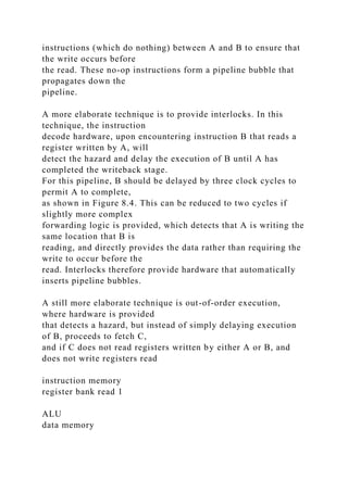
1. Consider the function compute variance listed below, which
computes the
variance of integer numbers stored in the array data.
1 int data[N];
2
3 int compute_variance() {
4 int sum1 = 0, sum2 = 0, result;
5 int i;
6
7 for(i=0; i < N; i++) {
8 sum1 += data[i];
9 }
10 sum1 /= N;
11
12 for(i=0; i < N; i++) {

13 sum2 += data[i] * data[i];
14 }
15 sum2 /= N;
16
17 result = (sum2 - sum1*sum1);
18
19 return result;
20 }
Suppose this program is executing on a 32-bit processor with a
direct-mapped cache
with parameters (m,S,E,B) = (32, 8, 1, 8). We make the
following additional
assumptions:
• An int is 4 bytes wide.
• sum1, sum2, result, and i are all stored in registers.
• data is stored in memory starting at address 0x0.
(a) Consider the case where N is 16. How many cache misses
will there be?
(b) Now suppose that N is 32. Recompute the number of cache
misses.
(c) Now consider executing for N = 16 on a 2-way set-
associative cache with
parameters (m,S,E,B) = (32, 8, 2, 4). In other words, the block
size is
halved, while there are two cache lines per set. How many cache
misses
would the code suffer?

EXERCISES
2. Recall from Section 9.2.3 that caches use the middle range of
address bits as the
set index and the high order bits as the tag. Why is this done?
How might cache
performance be affected if the middle bits were used as the tag
and the high order
bits were used as the set index?
3. Consider the C program and simplified memory map for a 16-
bit microcontroller
shown below. Assume that the stack grows from the top (area
D) and that the pro-
gram and static variables are stored in the bottom (area C) of
the data and program
memory region. Also, assume that the entire address space has
physical memory
associated with it.
interrupt vectors
data and program memory
0x0000
0x000F
0x0020
0xFFFF

A
C
D
memory-mapped I/O 0x0010
0x001FB
stack
program and static variables
1 #include <stdio.h>
2 #define FOO 0x0010
3 int n;
4 int* m;
5 void foo(int a) {
6 if (a > 0) {
7 n = n + 1;
8 foo(n);
9 }
10 }
11 int main() {
12 n = 0;
13 m = (int*)FOO;
14 foo(*m);
15 printf("n = %dn", n);
16 }
You may assume that in this system, an int is a 16-bit number,
that there is no op-
erating system and no memory protection, and that the program
has been compiled

and loaded into area C of the memory.
(a) For each of the variables n, m, and a, indicate where in
memory (region A, B,
C, or D) the variable will be stored.
(b) Determine what the program will do if the contents at
address 0x0010 is 0
upon entry.
(c) Determine what the program will do if the contents of
memory location 0x0010
is 1 upon entry.
4. Consider the following program:
1 int a = 2;
2 void foo(int b) {
3 printf("%d", b);
4 }
5 int main(void) {
6 foo(a);
7 a = 1;
8 }
Is it true or false that the value of a passed to foo will always be
2? Explain.
Assume that this is the entire program, that this program is

stored in persistent
memory, and that the program is executed on a bare-iron
microcontroller each time
a reset button is pushed.
10
Input and Output
10.1 I/O Hardware . . . . . . . . . . . . . . . . . . . . . . . . . . . . . 261
10.1.1 Pulse Width Modulation . . . . . . . . . . . . . . . . . . . . 262
10.1.2 General-Purpose Digital I/O . . . . . . . . . . . . . . . . . . 263
10.1.3 Serial Interfaces . . . . . . . . . . . . . . . . . . . . . . . . 267
10.1.4 Parallel Interfaces . . . . . . . . . . . . . . . . . . . . . . . . 270
10.1.5 Buses . . . . . . . . . . . . . . . . . . . . . . . . . . . . . . 271
10.2 Sequential Software in a Concurrent World . . . . . . . . . . . .
. 272
10.2.1 Interrupts and Exceptions . . . . . . . . . . . . . . . . . . . 273
Sidebar: Basics: Timers . . . . . . . . . . . . . . . . . . . . . . . . 275
10.2.2 Atomicity . . . . . . . . . . . . . . . . . . . . . . . . . . . . 276
10.2.3 Interrupt Controllers . . . . . . . . . . . . . . . . . . . . . . 277
10.2.4 Modeling Interrupts . . . . . . . . . . . . . . . . . . . . . . 278
10.3 Summary . . . . . . . . . . . . . . . . . . . . . . . . . . . . . . . . 283
Exercises . . . . . . . . . . . . . . . . . . . . . . . . . . . . . . . . . . . 284
Because cyber-physical systems integrate computing and
physical dynamics, the mech-
anisms in processors that support interaction with the outside
world are central to any
design. A system designer has to confront a number of issues.

Among these, the me-
chanical and electrical properties of the interfaces are
important. Incorrect use of parts,
such as drawing too much current from a pin, may cause a
system to malfunction or may
reduce its useful lifetime. In addition, in the physical world,
many things happen at once.
10. INPUT AND OUTPUT
Software, by contrast, is mostly sequential. Reconciling these
two disparate properties
is a major challenge, and is often the biggest risk factor in the
design of embedded sys-
tems. Incorrect interactions between sequential code and
concurrent events in the physical
world can cause dramatic system failures. In this chapter, we
deal with issues.
10.1 I/O Hardware
Embedded processors, be they microcontrollers, DSP
processors, or general-purpose pro-
cessors, typically include a number of input and output (I/O)
mechanisms on chip, ex-
posed to designers as pins of the chip. In this section, we review
some of the more
common interfaces provided, illustrating their properties
through the following running
example.
Example 10.1: Figure 10.1 shows an evaluation board for the
Luminary Micro
Stellaris R© microcontroller, which is an ARM CortexTM - M3

32-bit processor.
The microcontroller itself is in the center below the graphics
display. Many of the
pins of the microcontroller are available at the connectors
shown on either side of
the microcontroller and at the top and bottom of the board. Such
a board would
typically be used to prototype an embedded application, and in
the final product
it would be replaced with a custom circuit board that includes
only the hardware
required by the application. An engineer will develop software
for the board using
an integrated development environment (IDE) provided by the
vendor and load
the software onto flash memory to be inserted into the slot at
the bottom of the
board. Alternatively, software might be loaded onto the board
through the USB
interface at the top from the development computer.
The evaluation board in the above example is more than a
processor since it includes a
display and various hardware interfaces (switches and a
speaker, for example). Such a
board is often called a single-board computer or a
microcomputer board. We next
discuss a few of the interfaces provided by a microcontroller or
single-board computer.
For a more comprehensive description of the many kinds of I/O
interfaces in use, we
recommend Valvano (2007) and Derenzo (2003).

10.1. I/O HARDWARE
USB interface
JTAG and SWD interface
graphics
display
CAN bus interface
Ethernet interface
analog
(ADC)
inputs
micro-
controller
removable
�ash
memory
slot
PWM outputs
GPIO connectors
switches
connected
to GPIO pins

speaker
connected to
GPIO or PWM
Figure 10.1: Stellaris R© LM3S8962 evaluation board
(Luminary Micro R©, 2008a).
(Luminary Micro was acquired by Texas Instruments in 2009.)
10.1.1 Pulse Width Modulation
Pulse width modulation (PWM) is a technique for delivering a
variable amount of power
efficiently to external hardware devices. It can be used to
control for example the speed of
electric motors, the brightness of an LED light, and the
temperature of a heating element.
In general, it can deliver varying amounts of power to devices
that tolerate rapid and
abrupt changes in voltage and current.
PWM hardware uses only digital circuits, and hence is easy to
integrate on the same chip
with a microcontroller. Digital circuits, by design, produce only
two voltage levels, high
and low. A PWM signal rapidly switches between high and low
at some fixed frequency,
varying the amount of time that it holds the signal high. The
duty cycle is the proportion

of time that the voltage is high. If the duty cycle is 100%, then
the voltage is always high.
If the duty cycle is 0%, then the voltage is always low.
Many microcontrollers provide PWM peripheral devices (see
Figure 10.1). To use these,
a programmer typically writes a value to a memory-mapped
register to set the duty cycle
(the frequency may also be settable). The device then delivers
power to external hardware
in proportion to the specified duty cycle.
PWM is an effective way to deliver varying amounts of power,
but only to certain devices.
A heating element, for example, is a resistor whose temperature
increases as more cur-
rent passes through it. Temperature varies slowly, compared to
the frequency of a PWM
signal, so the rapidly varying voltage of the signal is averaged
out by the resistor, and the
temperature will be very close to constant for a fixed duty
cycle. Motors similarly aver-
age out rapid variations in input voltage. So do incandescent
and LED lights. Any device
whose response to changes in current or voltage is slow
compared to the frequency of the
PWM signal is a candidate for being controlled via PWM.
10.1.2 General-Purpose Digital I/O
Embedded system designers frequently need to connect
specialized or custom digital
hardware to embedded processors. Many embedded processors
have a number of general-
purpose I/O pins (GPIO), which enable the software to either
read or write voltage levels

representing a logical zero or one. If the processor supply
voltage is VDD, in active high
logic a voltage close to VDD represents a logical one, and a
voltage near zero represents
a logical zero. In active low logic, these interpretations are
reversed.
In many designs, a GPIO pin may be configured to be an output.
This enables software to
then write to a memory-mapped register to set the output
voltage to be either high or low.
By this mechanism, software can directly control external
physical devices.
However, caution is in order. When interfacing hardware to
GPIO pins, a designer needs
to understand the specifications of the device. In particular, the
voltage and current levels
vary by device. If a GPIO pin produces an output voltage of
VDD when given a logical
one, then the designer needs to know the current limitations
before connecting a device
to it. If a device with a resistance of R ohms is connected to it,
for example, then Ohm’s
law tells us that the output current will be
I = VDD/R .
10.1. I/O HARDWARE
It is essential to keep this current within specified tolerances.

Going outside these toler-
ances could cause the device to overheat and fail. A power
amplifier may be needed to
deliver adequate current. An amplifier may also be needed to
change voltage levels.
Example 10.2: The GPIO pins of the Luminary Micro Stellaris
R© microcon-
troller shown in Figure 10.1 may be configured to source or
sink varying amounts
of current up to 18 mA. There are restrictions on what
combinations of pins can
handle such relatively high currents. For example, Luminary
Micro R© (2008b)
states “The high-current GPIO package pins must be selected
such that there are
only a maximum of two per side of the physical package ... with
the total number
of high-current GPIO outputs not exceeding four for the entire
package.” Such
constraints are designed to prevent overheating of the device.
In addition, it may be important to maintain electrical isolation
between processor cir-
cuits and external devices. The external devices may have
messy (noisy) electrical char-
acteristics that will make the processor unreliable if the noise
spills over into the power
or ground lines of the processor. Or the external device may
operate in a very different
voltage or power regime compared to the processor. A useful
strategy is to divide a cir-
cuit into electrical domains, possibly with separate power
supplies, that have relatively
little influence on one another. Isolation devices such as opto-
isolators and transformers

may be used to enable communication across electrical domains.
The former convert an
electrical signal in one electrical domain into light, and detect
the light in the other elec-
trical domain and convert it back to an electrical signal. The
latter use inductive coupling
between electrical domains.
GPIO pins can also be configured as inputs, in which case
software will be able to react
to externally provided voltage levels. An input pin may be
Schmitt triggered, in which
case they have hysteresis, similar to the thermostat of Example
3.5. A Schmitt triggered
input pin is less vulnerable to noise. It is named after Otto H.
Schmitt, who invented it in
1934 while he was a graduate student studying the neural
impulse propagation in squid
nerves.
Example 10.3: The GPIO pins of the microcontroller shown in
Figure 10.1,
when configured as inputs, are Schmitt triggered.
In many applications, several devices may share a single
electrical connection. The de-
signer must take care to ensure that these devices do not
simultaneously drive the voltage
of this single electrical connection to different values, resulting

in a short circuit that can
cause overheating and device failure.
Example 10.4: Consider a factory floor where several
independent microcon-
trollers are all able to turn off a piece of machinery by asserting
a logical zero
on an output GPIO line. Such a design may provide additional
safety because
the microcontrollers may be redundant, so that failure of one
does not prevent
a safety-related shutdown from occurring. If all of these GPIO
lines are wired
together to a single control input of the piece of machinery,
then we have to take
precautions to ensure that the microcontrollers do not short each
other out. This
would occur if one microcontroller attempts to drive the shared
line to a high
voltage while another attempts to drive the same line to a low
voltage.
GPIO outputs may use open collector circuits, as shown in
Figure 10.2. In such a circuit,
writing a logical one into the (memory mapped) register turns
on the transistor, which
pulls the voltage on the output pin down to (near) zero. Writing
a logical zero into the
register turns off the transistor, which leaves the output pin
unconnected, or “open.”
A number of open collector interfaces may be connected as
shared line is connected to a pull-up resistor, which brings the
voltage of the line up to
VDD when all the transistors are turned off. If any one

transistor is turned on, then it will
bring the voltage of the entire line down to (near) zero without
creating a short circuit with
the other GPIO pins. Logically, all registers must have zeros in
them for the output to be
high. If any one of the registers has a one in it, then the output
will be low. Assuming
active high logic, the logical function being performed is NOR,
so such a circuit is called
a wired NOR. By varying the configuration, one can similarly
create wired OR or wired
AND.
10.1. I/O HARDWARE
microcontroller
register
drive
transistor
GPIO
pin
Figure 10.2: An open collector circuit for a GPIO pin.
microcontroller
microcontroller
microcontroller

register
drive
transistor
pull-up
resistor
VDD
GPIO pin
GPIO pin
GPIO pin
Figure 10.3: A number of open collector circuits wired together.
The term “open collector” comes from the name for the terminal
of a bipolar transistor. In
CMOS technologies, this type of interface will typically be
called an open drain interface.
It functions essentially in the same way.
Example 10.5: The GPIO pins of the microcontroller shown in
Figure 10.1,
when configured as outputs, may be specified to be open drain
circuits. They
may also optionally provide the pull-up resistor, which
conveniently reduces the
number of external discrete components required on a printed
circuit board.

DB-9 serial port DB-25 parallel port
USB IEEE 488
Figure 10.4: Connectors for serial and parallel interfaces.
GPIO outputs may also be realized with tristate logic, which
means that in addition to
producing an output high or low voltage, the pin may be simply
turned off. Like an open-
collector interface, this can facilitate sharing the same external
circuits among multiple
devices. Unlike an open-collector interface, a tristate design can
assert both high and low
voltages, rather than just one of the two.
10.1.3 Serial Interfaces
One of the key constraints faced by embedded processor
designers is the need to have
physically small packages and low power consumption. A
consequence is that the num-
ber of pins on the processor integrated circuit is limited. Thus,
each pin must be used
efficiently. In addition, when wiring together subsystems, the
number of wires needs to
be limited to keep the overall bulk and cost of the product in
check. Hence, wires must
also be used efficiently. One way to use pins and wires
efficiently is to send information
over them serially as sequences of bits. Such an interface is
called a serial interface.

A number of standards have evolved for serial interfaces so that
devices from different
manufacturers can (usually) be connected.
10.1. I/O HARDWARE
An old but persistent standard, RS-232, standardized by the
Electronics Industries Asso-
ciation (EIA), was first introduced in 1962 to connect teletypes
to modems. This standard
defines electrical signals and connector types; it persists
because of its simplicity and be-
cause of continued prevalence of aging industrial equipment
that uses it. The standard
defines how one device can transmit a byte to another device
asynchronously (meaning
that the devices do not share a clock signal). On older PCs, an
RS-232 connection may be
provided via a DB-9 connector, as shown in Figure 10.4. A
microcontroller will typically
use a universal asynchronous receiver/transmitter (UART) to
convert the contents of
an 8-bit register into a sequence of bits for transmission over an
RS-232 serial link.
For an embedded system designer, a major issue to consider is
that RS-232 interfaces can
be quite slow and may slow down the application software, if
the programmer is not very
careful.

Example 10.6: All variants of the Atmel AVR microcontroller
include a UART
that can be used to provide an RS-232 serial interface. To send
a byte over the
serial port, an application program may include the lines
1 while(!(UCSR0A & 0x20));
2 UDR0 = x;
where x is a variable of type uint8 t (a C data type specifying an
8-bit unsigned
integer). The symbols UCSR0A and UDR0 are defined in header
files provided in
the AVR IDE. They are defined to refer to memory locations
corresponding to
memory-mapped registers in the AVR architecture.
The first line above executes an empty while loop until the
serial transmit buffer
is empty. The AVR architecture indicates that the transmit
buffer is empty by
setting the sixth bit of the memory mapped register UCSR0A to
1. When that
bit becomes 1, the expression !(UCSR0A & 0x20) becomes 0
and the while
loop stops looping. The second line loads the value to be sent,
which is whatever
the variable x contains, into the memory-mapped register
UDR0.
Suppose you wish to send a sequence of 8 bytes stored in an
array x. You could
do this with the C code
1 for(i = 0; i < 8; i++) {

3 UDR0 = x[i];
4 }
How long would it take to execute this code? Suppose that the
serial port is set
to operate at 57600 baud, or bits per second (this is quite fast
for an RS-232
interface). Then after loading UDR0 with an 8-bit value, it will
take 8/57600
seconds or about 139 microseconds for the 8-bit value to be
sent. Suppose that
the frequency of the processor is operating at 18 MHz
(relatively slow for a mi-
crocontroller). Then except for the first time through the for
loop, each while
loop will need to consume approximately 2500 cycles, during
which time the
processor is doing no useful work.
To receive a byte over the serial port, a programmer may use
the following C
code:
2 return UDR0;
In this case, the while loop waits until the UART has received
an incoming

byte. The programmer must ensure that there will be an
incoming byte, or this
code will execute forever. If this code is again enclosed in a
loop to receive a
sequence of bytes, then the while loop will need to consume a
considerable
number of cycles each time it executes.
For both sending and receiving bytes over a serial port, a
programmer may use
an interrupt instead to avoid having an idle processor that is
waiting for the serial
communication to occur. Interrupts will be discussed below.
The RS-232 mechanism is very simple. The sender and receiver
first must agree on a
transmission rate (which is slow by modern standards). The
sender initiates transmission
of a byte with a start bit, which alerts the receiver that a byte is
coming. The sender then
clocks out the sequence of bits at the agreed-upon rate,
following them by one or two stop
bits. The receiver’s clock resets upon receiving the start bit and
is expected to track the
sender’s clock closely enough to be able to sample the incoming
signal sequentially and
recover the sequence of bits. There are many descendants of the
standard that support
higher rate communication, such as RS-422, RS-423, and more.
Newer devices designed to connect to personal computers
typically use universal serial
bus (USB) interfaces, standardized by a consortium of vendors.
USB 1.0 appeared in

10.1. I/O HARDWARE
1996 and supports a data rate of 12 Mbits/sec. USB 2.0
appeared in 2000 and supports
data rates up to 480 Mbits/sec. USB 3.0 appeared in 2008 and
supports data rates up to
4.8 Gbits/sec.
USB is electrically simpler than RS-232 and uses simpler, more
robust connectors, as
shown in Figure 10.4. But the USB standard defines much more
than electrical trans-
port of bytes, and more complicated control logic is required to
support it. Since modern
peripheral devices such as printers, disk drives, and audio and
video devices all include
microcontrollers, supporting the more complex USB protocol is
reasonable for these de-
vices.
Another serial interface that is widely implemented in
embedded processors is known
as JTAG (Joint Test Action Group), or more formally as the
IEEE 1149.1 standard test
access port and boundary-scan architecture. This interface
appeared in the mid 1980s
to solve the problem that integrated circuit packages and printed
circuit board technology
had evolved to the point that testing circuits using electrical
probes had become difficult or
impossible. Points in the circuit that needed to be accessed
became inaccessible to probes.

The notion of a boundary scan allows the state of a logical
boundary of a circuit (what
would traditionally have been pins accessible to probes) to be
read or written serially
through pins that are made accessible. Today, JTAG ports are
widely used to provide a
debug interface to embedded processors, enabling a PC-hosted
debugging environment
to examine and control the state of an embedded processor. The
JTAG port is used, for
example, to read out the state of processor registers, to set
breakpoints in a program, and
to single step through a program. A newer variant is serial wire
debug (SWD), which
provides similar functionality with fewer pins.
There are several other serial interfaces in use today, including
for example I2C (inter-
integrated circuit), SPI (serial peripheral interface bus), PCI
Express (peripheral compo-
nent interconnect express), FireWire, MIDI (musical instrument
digital interface), and
serial versions of SCSI (described below). Each of these has its
use. Also, network inter-
faces are typically serial.
10.1.4 Parallel Interfaces
A serial interface sends or receives a sequence of bits
sequentially over a single line. A
parallel interface uses multiple lines to simultaneously send
bits. Of course, each line
of a parallel interface is also a serial interface, but the logical
grouping and coordinated
action of these lines is what makes the interface a parallel
interface.

Historically, one of the most widely used parallel interfaces is
the IEEE-1284 printer port,
which on the IBM PC used a DB-25 connector, as shown in
Figure 10.4. This interface
originated in 1970 with the Centronics model 101 printer, and
hence is sometimes called
a Centronics printer port. Today, printers are typically
connected using USB or wireless
networks.
With careful programming, a group of GPIO pins can be used
together to realize a parallel
interface. In fact, embedded system designers sometimes find
themselves using GPIO
pins to emulate an interface not supported directly by their
hardware.
It seems intuitive that parallel interfaces should deliver higher
performance than serial
interfaces, because more wires are used for the interconnection.
However, this is not
necessarily the case. A significant challenge with parallel
interfaces is maintaining syn-
chrony across the multiple wires. This becomes more difficult
as the physical length of
the interconnection increases. This fact, combined with the
requirement for bulkier cables
and more I/O pins has resulted in many traditionally parallel

interfaces being replaced by
serial interfaces.
10.1.5 Buses
A bus is an interface shared among multiple devices, in contrast
to a point-to-point in-
terconnection linking exactly two devices. Busses can be serial
interfaces (such as USB)
or parallel interfaces. A widespread parallel bus is SCSI
(pronounced scuzzy, for small
computer system interface), commonly used to connect hard
drives and tape drives to
computers. Recent variants of SCSI interfaces, however, depart
from the traditional par-
allel interface to become serial interfaces. SCSI is an example
of a peripheral bus archi-
tecture, used to connect computers to peripherals such as sound
cards and disk drives.
Other widely used peripheral bus standards include the ISA bus
(industry standard archi-
tecture, used in the ubiquitous IBM PC architecture), PCI
(peripheral component inter-
face), and Parallel ATA (advanced technology attachment). A
somewhat different kind
of peripheral bus standard is IEEE-488, originally developed
more than 30 years ago to
connect automated test equipment to controlling computers.
This interface was designed
at Hewlett Packard and is also widely known as HP-IB (Hewlett
Packard interface bus)
and GPIB (general purpose interface bus). Many networks also
use a bus architecture.
Because a bus is shared among several devices, any bus

architecture must include a
media-access control (MAC) protocol to arbitrate competing
accesses. A simple MAC
10.2. SEQUENTIAL SOFTWARE IN A CONCURRENT
WORLD
protocol has a single bus master that interrogates bus slaves.
USB uses such a mech-
anism. An alternative is a time-triggered bus, where devices are
assigned time slots
during which they can transmit (or not, if they have nothing to
send). A third alternative
is a token ring, where devices on the bus must acquire a token
before they can use the
shared medium, and the token is passed around the devices
according to some pattern.
A fourth alternative is to use a bus arbiter, which is a circuit
that handles requests for
the bus according to some priorities. A fifth alternative is
carrier sense multiple access
(CSMA), where devices sense the carrier to determine whether
the medium is in use be-
fore beginning to use it, detect collisions that might occur when
they begin to use it, and
try again later when a collision occurs.
In all cases, sharing of the physical medium has implications on
the timing of applications.
Example 10.7: A peripheral bus provides a mechanism for

external devices to
communicate with a CPU. If an external device needs to transfer
a large amount
of data to the main memory, it may be inefficient and/or
disruptive to require the
CPU to perform each transfer. An alternative is direct memory
access (DMA).
In the DMA scheme used on the ISA bus, the transfer is
performed by a separate
device called a DMA controller which takes control of the bus
and transfers the
data. In some more recent designs, such as PCI, the external
device directly takes
control of the bus and performs the transfer without the help of
a dedicated DMA
controller. In both cases, the CPU is free to execute software
while the transfer is
occurring, but if the executed code needs access to the memory
or the peripheral
bus, then the timing of the program is disrupted by the DMA.
Such timing effects
can be difficult to analyze.
10.2 Sequential Software in a Concurrent World
As we saw in Example 10.6, when software interacts with the
external world, the tim-
ing of the execution of the software may be strongly affected.
Software is intrinsically
sequential, typically executing as fast as possible. The physical
world, however, is con-
current, with many things happening at once, and with the pace
at which they happen
determined by their physical properties. Bridging this mismatch
in semantics is one of

the major challenges that an embedded system designer faces. In
this section, we discuss
some of the key mechanisms for accomplishing this.
10.2.1 Interrupts and Exceptions
An interrupt is a mechanism for pausing execution of whatever
a processor is currently
doing and executing a pre-defined code sequence called an
interrupt service routine
(ISR) or interrupt handler. Three kinds of events may trigger an
interrupt. One is
a hardware interrupt, where some external hardware changes the
voltage level on an
interrupt request line. In the case of a software interrupt, the
program that is executing
triggers the interrupt by executing a special instruction or by
writing to a memory-mapped
register. A third variant is called an exception, where the
interrupt is triggered by internal
hardware that detects a fault, such as a segmentation fault.
For the first two variants, once the ISR completes, the program
that was interrupted re-
sumes where it left off. In the case of an exception, once the
ISR has completed, the pro-
gram that triggered the exception is not normally resumed.
Instead, the program counter
is set to some fixed location where, for example, the operating

system may terminate the
offending program.
Upon occurrence of an interrupt trigger, the hardware must first
decide whether to re-
spond. If interrupts are disabled, it will not respond. The
mechanism for enabling or
disabling interrupts varies by processor. Moreover, it may be
that some interrupts are
enabled and others are not. Interrupts and exceptions generally
have priorities, and an
interrupt will be serviced only if the processor is not already in
the middle of servicing
an interrupt with a higher priority. Typically, exceptions have
the highest priority and are
always serviced.
When the hardware decides to service an interrupt, it will
usually first disable interrupts,
push the current program counter and processor status
register(s) onto the stack, and
branch to a designated address that will normally contain a
jump to an ISR. The ISR must
store on the stack the values currently in any registers that it
will use, and restore their
values before returning from the interrupt, so that the
interrupted program can resume
where it left off. Either the interrupt service routine or the
hardware must also re-enable
interrupts before returning from the interrupt.

WORLD
Example 10.8: The ARM CortexTM - M3 is a 32-bit
microcontroller used in
industrial automation and other applications. It includes a
system timer called
SysTick. This timer can be used to trigger an ISR to execute
every 1ms. Suppose
for example that every 1ms we would like to count down from
some initial count
until the count reaches zero, and then stop counting down. The
following C code
defines an ISR that does this:
1 volatile uint timerCount = 0;
2 void countDown(void) {
3 if (timerCount != 0) {
4 timerCount--;
5 }
6 }
Here, the variable timerCount is a global variable, and it is
decremented each
time countDown() is invoked, until it reaches zero. We will
specify below
that this is to occur once per millisecond by registering
countDown() as an
ISR. The variable timerCount is marked with the C volatile
keyword, which
tells the compiler that the value of the variable will change at
unpredictable times
during execution of the program. This prevents the compiler
from performing
certain optimizations, such as caching the value of the variable
in a register and

reading it repeatedly. Using a C API provided by Luminary
Micro R© (2008c), we
can specify that countDown() should be invoked as an interrupt
service routine
once per millisecond as follows:
1 SysTickPeriodSet(SysCtlClockGet() / 1000);
2 SysTickIntRegister(&countDown);
3 SysTickEnable();
4 SysTickIntEnable();
The first line sets the number of clock cycles between “ticks” of
the SysTick
timer. The timer will request an interrupt on each tick.
SysCtlClockGet()
is a library procedure that returns the number of cycles per
second of the target
platform’s clock (e.g., 50,000,000 for a 50 MHz part). The
second line regis-
ters the ISR by providing a function pointer for the ISR (the
address of the
countDown() procedure). (Note: Some configurations do not
support run-
time registration of ISRs, as shown in this code. See the
documentation for your
particular system.) The third line starts the clock, enabling ticks
to occur. The
fourth line enables interrupts.

The timer service we have set up can be used, for example, to
perform some
function for two seconds and then stop. A program to do that is:
1 int main(void) {
2 timerCount = 2000;
3 ... initialization code from above ...
4 while(timerCount != 0) {
5 ... code to run for 2 seconds ...
6 }
7 }
Processor vendors provide many variants of the mechanisms
used in the previous exam-
ple, so you will need to consult the vendor’s documentation for
the particular processor
you are using. Since the code is not portable (it will not run
correctly on a different pro-
Basics: Timers
Microcontrollers almost always include some number of
peripheral devices called
timers. A programmable interval timer (PIT), the most common
type, simply counts
down from some value to zero. The initial value is set by
writing to a memory-mapped
register, and when the value hits zero, the PIT raises an
interrupt request. By writing to
a memory-mapped control register, a timer might be set up to
trigger repeatedly with-
out having to be reset by the software. Such repeated triggers
will be more precisely
periodic than what you would get if the ISR restarts the timer
each time it gets invoked.

This is because the time between when the count reaches zero in
the timer hardware
and the time when the counter gets restarted by the ISR is
difficult to control and vari-
able. For example, if the timer reaches zero at a time when
interrupts happen to be
disabled, then there will be a delay before the ISR gets invoked.
It cannot be invoked
before interrupts are re-enabled.
WORLD
cessor), it is wise to isolate such code from your application
logic and document carefully
what needs to be re-implemented to target a new processor.
10.2.2 Atomicity
An interrupt service routine can be invoked between any two
instructions of the main
program (or between any two instructions of a lower priority
ISR). One of the major chal-
lenges for embedded software designers is that reasoning about
the possible interleavings
of instructions can become extremely difficult. In the previous
example, the interrupt
service routine and the main program are interacting through a
shared variable, namely
timerCount. The value of that variable can change between any
two atomic opera-

tions of the main program. Unfortunately, it can be quite
difficult to know what operations
are atomic. The term “atomic” comes from the Greek work for
“indivisible,” and it is far
from obvious to a programmer what operations are indivisible.
If the programmer is writ-
ing assembly code, then it may be safe to assume that each
assembly language instruction
is atomic, but many ISAs include assembly level instructions
that are not atomic.
Example 10.9: The ARM instruction set includes a LDM
instruction, which
loads multiple registers from consecutive memory locations. It
can be interrupted
part way through the loads (ARM Limited, 2006).
At the level of a C program, it can be even more difficult to
know what operations are
atomic. Consider a single, innocent looking statement
timerCount = 2000;
On an 8-bit microcontroller, this statement may take more than
one instruction cycle to
execute (an 8-bit word cannot store both the instruction and the
constant 2000; in fact, the
constant alone does not fit in an 8-bit word). An interrupt could
occur part way through the
execution of those cycles. Suppose that the ISR also writes to
the variable timerCount.
In this case, the final value of the timerCount variable may be
composed of 8 bits set
in the ISR and the remaining bits set by the above line of C, for
example. The final
value could be very different from 2000, and also different from

the value specified in the
interrupt service routine. Will this bug occur on a 32-bit
microcontroller? The only way
to know for sure is to fully understand the ISA and the
compiler. In such circumstances,
there is no advantage to having written the code in C instead of
assembly language.
Bugs like this in a program are extremely difficult to identify
and correct. Worse, the
problematic interleavings are quite unlikely to occur, and hence
may not show up in test-
ing. For safety-critical systems, programmers have to make
every effort to avoid such
bugs. One way to do this is to build programs using higher-level
computation, as discussed in Chapter 6. Of course, the
implementation of those models
of computation needs to be correct, but presumably, that
implementation is constructed
by experts in concurrency, rather than by application engineers.
When working at the level of C and ISRs, a programmer must
carefully reason about
the order of operations. Although many interleavings are
possible, operations given as a
sequence of C statements must execute in order (more precisely,
they must behave as if

they had executed in order, even if out-of-order execution is
used).
Example 10.10: In example 10.8, the programmer can rely on
the statements
within main() executing in order. Notice that in that example,
the statement
timerCount = 2000;
appears before
SysTickIntEnable();
The latter statement enables the SysTick interrupt. Hence, the
former statement
cannot be interrupted by the SysTick interrupt.
10.2.3 Interrupt Controllers
An interrupt controller is the logic in the processor that handles
interrupts. It supports
some number of interrupts and some number of priority levels.
Each interrupt has an
interrupt vector, which is the address of an ISR or an index into
an array called the
interrupt vector table that contains the addresses of all the ISRs.
WORLD

Example 10.11: The Luminary Micro LM3S8962 controller,
shown in Figure
10.1, includes an ARM CortexTM - M3 core microcontroller
that supports 36 in-
terrupts with eight priority levels. If two interrupts are assigned
the same priority
number, then the one with the lower vector will have priority
over the one with
the higher vector.
When an interrupt is asserted by changing the voltage on a pin,
the response may be either
level triggered or edge triggered. For level-triggered interrupts,
the hardware asserting
the interrupt will typically hold the voltage on the line until it
gets an acknowledgement,
which indicates that the interrupt is being handled. For edge-
triggered interrupts, the
hardware asserting the interrupt changes the voltage for only a
short time. In both cases,
open collector lines can be used so that the same physical line
can be shared among
several devices (of course, the ISR will require some
mechanism to determine which
device asserted the interrupt, for example by reading a memory-
mapped register in each
device that could have asserted the interrupt).
Sharing interrupts among devices can be tricky, and careful
consideration must be given to
prevent low priority interrupts from blocking high priority
interrupts. Asserting interrupts
by writing to a designated address on a bus has the advantage
that the same hardware can
support many more distinct interrupts, but the disadvantage that
peripheral devices get

more complex. The peripheral devices have to include an
interface to the memory bus.
10.2.4 Modeling Interrupts
The behavior of interrupts can be quite difficult to fully
understand, and many catastrophic
system failures are caused by unexpected behaviors.
Unfortunately, the logic of interrupt
controllers is often described in processor documentation very
imprecisely, leaving many
possible behaviors unspecified. One way to make this logic
more precise is to model it as
an FSM.
Example 10.12: The program of Example 10.8, which performs
some action
for two seconds, is shown in Figure 10.5 together with two
finite state machines
volatile uint timerCount = 0;
void ISR(void) {
… disable interrupts
if(timerCount != 0) {
timerCount--;
}
… enable interrupts
}
int main(void) {

// initialization code
SysTickIntRegister(&ISR);
… // other init
timerCount = 2000;
while(timerCount != 0) {
… code to run for 2 seconds
}
}
… whatever comes next
E
D
A
B
C
Figure 10.5: State machine models and main program for a
program that does
something for two seconds and then continues to do something
else.
WORLD
that model the ISR and the main program. The states of the
FSMs correspond to
positions in the execution labeled A through E, as shown in the
program listing.
These positions are between C statements, so we are assuming

here that these
statements are atomic operations (a questionable assumption in
general).
We may wish to determine whether the program is assured of
always reaching
position C. In other words, can we assert with confidence that
the program will
eventually move beyond whatever computation it was to
perform for two sec-
onds? A state machine model will help us answer that question.
The key question now becomes how to compose these state
machines to correctly
model the interaction between the two pieces of sequential code
in the proce-
dures ISR and main. It is easy to see that asynchronous
composition is not the
right choice because the interleavings are not arbitrary. In
particular, main can
be interrupted by ISR, but ISR cannot be interrupted by main.
Asynchronous
composition would fail to capture this asymmetry.
Assuming that the interrupt is always serviced immediately
upon being requested,
we wish to have a model something like that shown in Figure
10.6. In that figure,
a two-state FSM models whether an interrupt is being serviced.
The transition
from Inactive to Active is triggered by a pure input assert,
which models the timer
hardware requesting interrupt service. When the ISR completes
its execution,
another pure input return triggers a return to the Inactive state.
Notice here that

the transition from Inactive to Active is a preemptive transition,
indicated by the
small circle at the start of the transition, suggesting that it
should be taken im-
mediately when assert occurs, and that it is a reset transition,
suggesting that the
state refinement of Active should begin in its initial state upon
entry.
If we combine Figures 10.5 and 10.6 we get the hierarchical
FSM in Figure 10.7.
Notice that the return signal is both an input and an output now.
It is an output
produced by the state refinement of Active, and it is an input to
the top-level FSM,
where it triggers a transition to Inactive. Having an output that
is also an input
provides a mechanism for a state refinement to trigger a
transition in its container
state machine.
To determine whether the program reaches state C, we can study
the flattened
state machine shown in Figure 10.8. Studying that machine
carefully, we see that
in fact there is no assurance that state C will be reached! If, for
example, assert
is present on every reaction, then C is never reached.

E
D
A
B
C
Figure 10.6: Sketch of a state machine model for the interaction
between an ISR
and the main program.
Could this happen in practice? With this program, it is
improbable, but not im-
possible. It could happen if the ISR itself takes longer to
execute than the time
between interrupts. Is there any assurance that this will not
happen? Unfortu-
nately, our only assurance is a vague notion that processors are
faster than that.
There is no guarantee.
In the above example, modeling the interaction between a main
program and an interrupt
service routine exposes a potential flaw in the program.
Although the flaw may be unlikely
to occur in practice in this example, the fact that the flaw is
present at all is disturbing.
In any case, it is better to know that the flaw is present, and to
decide that the risk is
acceptable, than to not know it is present.
Interrupt mechanisms can be quite complex. Software that uses
these mechanisms to
provide I/O to an external device is called a device driver.
Writing device drivers that

are correct and robust is a challenging engineering task
requiring a deep understanding
WORLD
Figure 10.7: Hierarchical state machine model for the
interaction between an ISR
and the main program.
Figure 10.8: Flattened version of the hierarchical state machine
in Figure 10.7.
of the architecture and considerable skill reasoning about
concurrency. Many failures in
computer systems are caused by unexpected interactions
between device drivers and other
programs.
10.3 Summary
This chapter has reviewed hardware and software mechanisms
used to get sensor data
into processors and commands from the processor to actuators.

The emphasis is on un-
derstanding the principles behind the mechanisms, with a
particular focus on the bridging
between the sequential world of software and the parallel
physical world.
EXERCISES
Exercises
1. Similar to Example 10.6, consider a C program for an Atmel
AVR that uses a UART
to send 8 bytes to an RS-232 serial interface, as follows:
1 for(i = 0; i < 8; i++) {
3 UDR0 = x[i];
4 }
Assume the processor runs at 50 MHz; also assume that initially
the UART is idle,
so when the code begins executing, UCSR0A & 0x20 == 0x20 is
true; further,
assume that the serial port is operating at 19,200 baud. How
many cycles are re-
quired to execute the above code? You may assume that the for
statement executes
in three cycles (one to increment i, one to compare it to 8, and
one to perform the
conditional branch); the while statement executes in 2 cycles
(one to compute

!(UCSR0A & 0x20) and one to perform the conditional branch);
and the assig-
ment to UDR0 executes in one cycle.
2. Figure 10.9 gives the sketch of a program for an Atmel AVR
microcontroller that
performs some function repeatedly for three seconds. The
function is invoked by
calling the procedure foo(). The program begins by setting up a
timer interrupt
to occur once per second (the code to do this setup is not
shown). Each time the
interrupt occurs, the specified interrupt service routine is called.
That routine decre-
ments a counter until the counter reaches zero. The main()
procedure initializes the
counter with value 3 and then invokes foo() until the counter
reaches zero.
(a) We wish to assume that the segments of code in the grey
boxes, labeled A, B,
and C, are atomic. State conditions that make this assumption
valid.
(b) Construct a state machine model for this program, assuming
as in part (a)
that A, B, and C, are atomic. The transitions in your state
machine should
be labeled with “guard/action”, where the action can be any of
A, B, C, or
nothing. The actions A, B, or C should correspond to the
sections of code in
the grey boxes with the corresponding labels. You may assume
these actions
are atomic.

(c) Is your state machine deterministic? What does it tell you
about how many
times foo() may be invoked? Do all the possible behaviors of
your model
correspond to what the programmer likely intended?
#include <avr/interrupt.h>
volatile uint16_t timer_count = 0;
// Interrupt service routine.
SIGNAL(SIG_OUTPUT_COMPARE1A) {
if(timer_count > 0) {
timer_count--;
}
}
// Main program.
int main(void) {
// Set up interrupts to occur
// once per second.
...
// Start a 3 second timer.
timer_count = 3;
// Do something repeatedly
// for 3 seconds.
while(timer_count > 0) {

foo();
}
}
A
B
C
Figure 10.9: Sketch of a C program that performs some function
by calling proce-
dure foo() repeatedly for 3 seconds, using a timer interrupt to
determine when to
stop.
EXERCISES
Note that there are many possible answers. Simple models are
preferred over elab-
orate ones, and complete ones (where everything is defined)
over incomplete ones.
Feel free to give more than one model.
3. In a manner similar to example 10.8, create a C program for
the ARM CortexTM -
M3 to use the SysTick timer to invoke a system-clock ISR with
a jiffy interval of
10 ms that records the time since system start in a 32-bit int.
How long can this
program run before your clock overflows?

4. Consider a dashboard display that displays “normal” when
brakes in the car operate
normally and “emergency” when there is a failure. The intended
behavior is that
once “emergency” has been displayed, “normal” will not again
be displayed. That
is, “emergency” remains on the display until the system is reset.
In the following code, assume that the variable display defines
what is displayed.
Whatever its value, that is what appears on the dashboard.
1 volatile static uint8_t alerted;
2 volatile static char* display;
3 void ISRA() {
4 if (alerted == 0) {
5 display = "normal";
6 }
7 }
8 void ISRB() {
9 display = "emergency";
10 alerted = 1;
11 }
12 void main() {
13 alerted = 0;
14 ...set up interrupts...
15 ...enable interrupts...
16 ...
17 }
Assume that ISRA is an interrupt service routine that is invoked
when the brakes
are applied by the driver. Assume that ISRB is invoked if a
sensor indicates that the

brakes are being applied at the same time that the accelerator
pedal is depressed.
Assume that neither ISR can interrupt itself, but that ISRB has
higher priority than
ISRA, and hence ISRB can interrupt ISRA, but ISRA cannot
interrupt ISRB.
Assume further (unrealistically) that each line of code is
atomic.
(a) Does this program always exhibit the intended behavior?
Explain. In the
remaining parts of this problem, you will construct various
models that will
either demonstrate that the behavior is correct or will illustrate
how it can be
incorrect.
(b) Construct a determinate extended state machine modeling
ISRA. Assume
that:
• alerted is a variable of type {0, 1} ⊂ uint8 t,
• there is a pure input A that when present indicates an interrupt
request for
ISRA, and
• display is an output of type char*.
(c) Give the size of the state space for your solution.

(d) Explain your assumptions about when the state machine in
(b) reacts. Is this
time triggered, event triggered, or neither?
(e) Construct a determinate extended state machine modeling
ISRB. This one has
a pure input B that when present indicates an interrupt request
for ISRB.
(f) Construct a flat (non-hierarchical) determinate extended
state machine de-
scribing the joint operation of the these two ISRs. Use your
model to argue
the correctness of your answer to part (a).
(g) Give an equivalent hierarchical state machine. Use your
model to argue the
correctness of your answer to part (a).
5. Suppose a processor handles interrupts as specified by the
following FSM:
EXERCISES
Here, we assume a more complicated interrupt controller than
that considered in
Example 10.12, where there are several possible interrupts and
an arbiter that de-
cides which interrupt to service. The above state machine shows
the state of one

interrupt. When the interrupt is asserted, the FSM transitions to
the Pending state,
and remains there until the arbiter provides a handle input. At
that time, the FSM
transitions to the Active state and produces an acknowledge
output. If another inter-
rupt is asserted while in the Active state, then it transitions to
Active and Pending.
When the ISR returns, the input return causes a transition to
either Inactive or Pend-
ing, depending on the starting point. The deassert input allows
external hardware
to cancel an interrupt request before it gets serviced.
Answer the following questions.
(a) If the state is Pending and the input is return, what is the
reaction?
(b) If the state is Active and the input is assert ∧ deassert, what
is the reaction?
(c) Suppose the state is Inactive and the input sequence in three
successive reac-
tions is:
i. assert ,
ii. deassert ∧ handle ,
iii. return .

What are all the possible states after reacting to these inputs?
Was the interrupt
handled or not?
(d) Suppose that an input sequence never includes deassert. Is it
true that every
assert input causes an acknowledge output? In other words, is
every interrupt
request serviced? If yes, give a proof. If no, give a
counterexample.
6. Suppose you are designing a processor that will support two
interrupts whose logic
is given by the FSM in Exercise 5. Design an FSM giving the
logic of an arbiter
that assigns one of these two interrupts higher priority than the
other. The inputs
should be the following pure signals:
assert1, return1, assert2, return2
to indicate requests and return from interrupt for interrupts 1
and 2, respectively.
The outputs should be pure signals handle1 and handle2.
Assuming the assert
inputs are generated by two state machines like that in Exercise
5, can you be sure
that this arbiter will handle every request that is made? Justify
your answer.
7. Consider the following program that monitors two sensors.
Here sensor1 and
sensor2 denote the variables storing the readouts from two
sensors. The actual

read is performed by the functions readSensor1() and
readSensor2(), re-
spectively, which are called in the interrupt service routine ISR.
1 char flag = 0;
2 volatile char* display;
3 volatile short sensor1, sensor2;
4
5 void ISR() {
6 if (flag) {
7 sensor1 = readSensor1();
8 } else {
9 sensor2 = readSensor2();
10 }
11 }
12
13 int main() {
14 // ... set up interrupts ...
15 // ... enable interrupts ...
16 while(1) {
17 if (flag) {
18 if isFaulty2(sensor2) {
19 display = "Sensor2 Faulty";
20 }
EXERCISES
21 } else {

22 if isFaulty1(sensor1) {
23 display = "Sensor1 Faulty";
24 }
25 }
26 flag = !flag;
27 }
28 }
Functions isFaulty1() and isFaulty2() check the sensor readings
for any
discrepancies, returning 1 if there is a fault and 0 otherwise.
Assume that the vari-
able display defines what is shown on the monitor to alert a
human operator
about faults. Also, you may assume that flag is modified only in
the body of
main.
(a) Is it possible for the ISR to update the value of sensor1
while the main
function is checking whether sensor1 is faulty? Why or why
not?
(b) Suppose a spurious error occurs that causes sensor1 or
sensor2 to be a
faulty value for one measurement. Is it possible for that this
code would not
report “Sensor1 faulty” or “Sensor2 faulty”?
(c) Assuming the interrupt source for ISR() is timer-driven,
what conditions
would cause this code to never check whether the sensors are
faulty?

(d) Suppose that instead being interrupt driven, ISR and main
are executed con-
currently, each in its own thread. Assume a microkernel that can
interrupt
any thread at any time and switch contexts to execute another
thread. In this
scenario, is it possible for the ISR to update the value of
sensor1 while the
main function is checking whether sensor1 is faulty? Why or
why not?
11
Multitasking
11.1 Imperative Programs . . . . . . . . . . . . . . . . . . . . . . . . . 294
Sidebar: Linked Lists in C . . . . . . . . . . . . . . . . . . . . . . . 297
11.2 Threads . . . . . . . . . . . . . . . . . . . . . . . . . . . . . . . . . 298
11.2.1 Creating Threads . . . . . . . . . . . . . . . . . . . . . . . . 298
11.2.2 Implementing Threads . . . . . . . . . . . . . . . . . . . . . 301
11.2.3 Mutual Exclusion . . . . . . . . . . . . . . . . . . . . . . . . 302
11.2.4 Deadlock . . . . . . . . . . . . . . . . . . . . . . . . . . . . 305
Sidebar: Operating Systems . . . . . . . . . . . . . . . . . . . . . . 306
11.2.5 Memory Consistency Models . . . . . . . . . . . . . . . . . 308
11.2.6 The Problem with Threads . . . . . . . . . . . . . . . . . . . 309
11.3 Processes and Message Passing . . . . . . . . . . . . . . . . . . . .
311
11.4 Summary . . . . . . . . . . . . . . . . . . . . . . . . . . . . . . . . 316
Exercises . . . . . . . . . . . . . . . . . . . . . . . . . . . . . . . . . . . 318

In this chapter, we discuss mid-level mechanisms that are used
in software to provide
concurrent execution of sequential code. There are a number of
reasons for executing
multiple sequential programs concurrently, but they all involve
timing. One reason is to
improve responsiveness by avoiding situations where long-
running programs can block a
program that responds to external stimuli, such as sensor data or
a user request. Improved
responsiveness reduces latency, the time between the occurrence
of a stimulus and the
response. Another reason is to improve performance by
allowing a program to run simul-
11. MULTITASKING
Concurrent model of computation
dataflow, time triggered, synchronous, etc.
Multitasking
processes, threads, message passing
Processor
interrupts, pipelining, multicore, etc.
Figure 11.1: Layers of abstraction for concurrency in programs.
taneously on multiple processors or cores. This is also a timing
issue, since it presumes
that it is better to complete tasks earlier than later. A third

reason is to directly control
the timing of external interactions. A program may need to
perform some action, such as
updating a display, at particular times, regardless of what other
tasks might be executing
at that time.
We have already discussed concurrency in a variety of contexts.
Figure 11.1 shows the re-
lationship between the subject of this chapter and those of other
chapters. Chapters 8 and
10 cover the lowest layer in Figure 11.1, which represents how
hardware provides con-
current mechanisms to the software designer. Chapters 5 and 6
cover the highest layer,
which consists of abstract models of concurrency, including
synchronous composition,
dataflow, and time-triggered models. This chapter bridges these
two layers. It describes
mechanisms that are implemented using the low-level
mechanisms and can provide infras-
tructure for realizing the high-level mechanisms. Collectively,
these mid-level techniques
are called multitasking, meaning the simultaneous execution of
multiple tasks.
Embedded system designers frequently use these mid-level
mechanisms directly to build
applications, but it is becoming increasingly common for
designers to use instead the
high-level mechanisms. The designer constructs a model using a
software tool that sup-
ports a model of computation (or several models of
computation). The model is then
automatically or semi-automatically translated into a program
that uses the mid-level or

11. MULTITASKING
1 #include <stdlib.h>
3 int x; // Value that gets updated.
4 typedef void notifyProcedure(int); // Type of notify proc.
5 struct element {
6 notifyProcedure* listener; // Pointer to notify procedure.
7 struct element* next; // Pointer to the next item.
8 };
9 typedef struct element element_t; // Type of list elements.
10 element_t* head = 0; // Pointer to start of list.
11 element_t* tail = 0; // Pointer to end of list.
12
13 // Procedure to add a listener.
14 void addListener(notifyProcedure* listener) {
15 if (head == 0) {
16 head = malloc(sizeof(element_t));
17 head->listener = listener;
18 head->next = 0;
19 tail = head;
20 } else {
21 tail->next = malloc(sizeof(element_t));
22 tail = tail->next;
23 tail->listener = listener;
24 tail->next = 0;
25 }
26 }

27 // Procedure to update x.
28 void update(int newx) {
29 x = newx;
30 // Notify listeners.
31 element_t* element = head;
32 while (element != 0) {
33 (*(element->listener))(newx);
34 element = element->next;
35 }
36 }
37 // Example of notify procedure.
38 void print(int arg) {
39 printf("%d ", arg);
40 }
Figure 11.2: A C program used in a series of examples in this
chapter.
11.1. IMPERATIVE PROGRAMS
low-level mechanisms. This translation process is variously
called code generation or
autocoding.
The mechanisms described in this chapter are typically provided
by an operating system,
a microkernel, or a library of procedures. They can be rather
tricky to implement cor-
rectly, and hence the implementation should be done by experts
(for some of the pitfalls,
see Boehm (2005)). Embedded systems application programmers

often find themselves
having to implement such mechanisms on bare iron (a processor
without an operating
system). Doing so correctly requires deep understanding of
concurrency issues.
This chapter begins with a brief description of models for
sequential programs, which
enable models of concurrent compositions of such sequential
programs. We then progress
to discuss threads, processes, and message passing, which are
three styles of composition
of sequential programs.
11.1 Imperative Programs
A programming language that expresses a computation as a
sequence of operations is
called an imperative language. C is an imperative language.
Example 11.1: In this chapter, we illustrate several key points
using the example
C program shown in Figure 11.2. This program implements a
commonly used
design pattern called the observer pattern (Gamma et al., 1994).
In this pattern,
an update procedure changes the value of a variable x.
Observers (which are
other programs or other parts of the program) will be notified
whenever x is
changed by calling a callback procedure. For example, the value
of x might be
displayed by an observer on a screen. Whenever the value
changes, the observer
needs to be notified so that it can update the display on the
screen. The following

main procedure uses the procedures defined in Figure 11.2:
1 int main(void) {
2 addListener(&print);
4 update(1);
6 update(2);
7 return 0;
8 }
11. MULTITASKING
This test program registers the print procedure as a callback
twice, then per-
forms an update (setting x = 1), then registers the print
procedure again, and
finally performs another update (setting x = 2). The print
procedure simply
prints the current value, so the output when executing this test
program is 1 1 2
2 2.
A C program specifies a sequence of steps, where each step
changes the state of the
memory in the machine. In C, the state of the memory in the
machine is represented by
the values of variables.
Example 11.2: In the program in Figure 11.2, the state of the
memory of the

machine includes the value of variable x (which is a global
variable) and a list of
elements pointed to by the variable head (another global
variable). The list itself
is represented as a linked list, where each element in the list
contains a function
pointer referring to a procedure to be called when x changes.
During execution of the C program, the state of the memory of
the machine will
need to include also the state of the stack, which includes any
local variables.
Using extended state machines, we can model the execution of
certain simple C programs,
assuming the programs have a fixed and bounded number of
variables. The variables of
the C program will be the variables of the state machine. The
states of the state machine
will represent positions in the program, and the transitions will
represent execution of the
program.
Example 11.3: Figure 11.3 shows a model of the update
procedure in Figure
11.2. The machine transitions from the initial Idle state when
the update proce-
dure is called. The call is signaled by the input arg being
present; its value will be
the int argument to the update procedure. When this transition is
taken, newx
(on the stack) will be assigned the value of the argument. In
addition, x (a global
variable) will be updated.

11.1. IMPERATIVE PROGRAMS
Figure 11.3: Model of the update procedure in Figure 11.2.
After this first transition, the machine is in state 31,
corresponding to the program
counter position just prior to the execution of line 31 in Figure
11.2. It then
unconditionally transitions to state 32 and sets the value of
element. From state
32, there are two possibilities; if element = 0, then the machine
transitions back
to Idle and produces the pure output return. Otherwise, it
transitions to 33.
On the transition from 33 to 34, the action is a procedure call to
the listener with
the argument being the stack variable newx. The transition from
34 back to 32
occurs upon receiving the pure input returnFromListener, which
indicates that the
listener procedure returns.
The model in Figure 11.3 is not the only model we could have
constructed of the update
procedure. In constructing such a model, we need to decide on
the level of detail, and we
need to decide which actions can be safely treated as atomic
operations. Figure 11.3 uses

11. MULTITASKING
Linked Lists in C
A linked list is a data structure for storing a list of elements that
varies in length during
execution of a program. Each element in the list contains a
payload (the value of the
element) and a pointer to the next element in the list (or a null
pointer if the element is
the last one). For the program in Figure 11.2, the linked list
data structure is defined
by:
1 typedef void notifyProcedure(int);
2 struct element {
3 notifyProcedure* listener;
4 struct element* next;
5 };
6 typedef struct element element_t;
7 element_t* head = 0;
8 element_t* tail = 0;
The first line declares that notifyProcedure is a type whose
value is a C procedure
that takes an int and returns nothing. Lines 2–5 declare a struct,
a composite data
type in C. It has two pieces, listener (with type
notifyProcedure*, which is
a function pointer, a pointer to a C procedure) and next (a
pointer to an instance of
the same struct). Line 6 declares that element t is a type
referring to an instance of

the structure element.
Line 7 declares head, a pointer to a list element. It is initialized
to 0, a value that
indicates an empty list. The addListener procedure in Figure
11.2 creates the first
list element using the following code:
3 head->next = 0;
4 tail = head;
Line 1 allocates memory from the heap using malloc to store a
list element and
sets head to point to that element. Line 2 sets the payload of the
element, and line 3
indicates that this is the last element in the list. Line 4 sets tail,
a pointer to the last
list element. When the list is not empty, the addListener
procedure will use the
tail pointer rather than head to append an element to the list.
11.2. THREADS
lines of code as a level of detail, but there is no assurance that a
line of C code executes
atomically (it usually does not).
In addition, accurate models of C programs are often not finite
state systems. Considering

only the code in Figure 11.2, a finite-state model is not
appropriate because the code
supports adding an arbitrary number of listeners to the list. If
we combine Figure 11.2
with the main procedure in Example 11.1, then the system is
finite state because only
three listeners are put on the list. An accurate finite-state
model, therefore, would need to
include the complete program, making modular reasoning about
the code very difficult.
The problems get much worse when we add concurrency to the
mix. We will show in
this chapter that accurate reasoning about C programs with mid-
level concurrency mech-
anisms such as threads is astonishingly difficult and error
prone. It is for this reason that
designers are tending towards the upper layer in Figure 11.1.
11.2 Threads
Threads are imperative programs that run concurrently and
share a memory space. They
can access each others’ variables. Many practitioners in the
field use the term “threads”
more narrowly to refer to particular ways of constructing
programs that share memory, but
here we will use the term broadly to refer to any mechanism
where imperative programs
run concurrently and share memory. In this broad sense, threads
exist in the form of
interrupts on almost all microprocessors, even without any
operating system at all (bare
iron).
11.2.1 Creating Threads

Most operating systems provide a higher-level mechanism than
interrupts to realize im-
perative programs that share memory. The mechanism is
provided in the form of a col-
lection of procedures that a programmer can use. Such
procedures typically conform to
a standardized API (application program interface), which
makes it possible to write
programs that are portable (they will run on multiple processors
and/or multiple operating
systems). Pthreads (or POSIX threads) is such an API; it is
integrated into many modern
operating systems. Pthreads defines a set of C programming
language types, functions and
constants. It was standardized by the IEEE in 1988 to unify
variants of Unix. In Pthreads,
11. MULTITASKING
1 #include <pthread.h>
3 void* printN(void* arg) {
4 int i;
5 for (i = 0; i < 10; i++) {
6 printf("My ID: %dn", *(int*)arg);
7 }
8 return NULL;
9 }
10 int main(void) {

11 pthread_t threadID1, threadID2;
12 void* exitStatus;
13 int x1 = 1, x2 = 2;
14 pthread_create(&threadID1, NULL, printN, &x1);
15 pthread_create(&threadID2, NULL, printN, &x2);
16 printf("Started threads.n");
17 pthread_join(threadID1, &exitStatus);
19 return 0;
20 }
Figure 11.4: Simple multithreaded C program using Pthreads.
a thread is defined by a C procedure and created by invoking
the pthread create
procedure.1
Example 11.4: A simple multithreaded C program using
Pthreads is shown in
Figure 11.4. The printN procedure (lines 3–9) — the procedure
that the thread
begins executing — is called the start routine; in this case, the
start routine
prints the argument passed to it 10 times and then exits, which
will cause the
thread to terminate. The main procedure creates two threads,
each of which will
execute the start routine. The first one, created on line 14, will
print the value
1. The second one, created on line 15, will print the value 2.
When you run this
1For brevity, in the examples in this text we do not check for
failures, as any well-written program using
Pthreads should. For example, pthread create will return 0 if it
succeeds, and a non-zero error code if

it fails. It could fail, for example, due to insufficient system
resources to create another thread. Any program
that uses pthread create should check for this failure and handle
it in some way. Refer to the Pthreads
documentation for details.
11.2. THREADS
program, values 1 and 2 will be printed in some interleaved
order that depends
on the thread scheduler. Typically, repeated runs will yield
different interleaved
orders of 1’s and 2’s.
The pthread create procedure creates a thread and returns
immediately. The
start routine may or may not have actually started running when
it returns. Lines
17 and 18 use pthread join to ensure that the main program does
not ter-
minate before the threads have finished. Without these two
lines, running the
program may not yield any output at all from the threads.
A start routine may or may not return. In embedded
applications, it is quite common to
define start routines that never return. For example, the start
routine might execute forever
and update a display periodically. If the start routine does not
return, then any other thread
that calls its pthread join will be blocked indefinitely.

As shown in Figure 11.4, the start routine can be provided with
an argument and can
return a value. The fourth argument to pthread create is the
address of the argument
to be passed to the start routine. It is important to understand
the memory model of C,
explained in Section 9.3.5, or some very subtle errors could
occur, as illustrated in the
next example.
Example 11.5: Suppose we attempt to create a thread inside a
procedure like
this:
1 pthread_t createThread(int x) {
2 pthread_t ID;
3 pthread_create(&ID, NULL, printN, &x);
4 return ID;
5 }
This code would be incorrect because the argument to the start
routine is given by
a pointer to a variable on the stack. By the time the thread
accesses the specified
memory address, the createThread procedure will likely have
returned and
the memory address will have been overwritten by whatever
went on the stack
next.

11. MULTITASKING
11.2.2 Implementing Threads
The core of an implementation of threads is a scheduler that
decides which thread to
execute next when a processor is available to execute a thread.
The decision may be
based on fairness, where the principle is to give every active
thread an equal opportunity
to run, on timing constraints, or on some measure of importance
or priority. Scheduling
algorithms are discussed in detail in Chapter 12. In this section,
we simply describe how
a thread scheduler will work without worrying much about how
it makes a decision on
which thread to execute.
The first key question is how and when the scheduler is
invoked. A simple technique
called cooperative multitasking does not interrupt a thread
unless the thread itself calls
a certain procedure or one of a certain set of procedures. For
example, the scheduler may
intervene whenever any operating system service is invoked by
the currently executing
thread. An operating system service is invoked by making a call
to a library procedure.
Each thread has its own stack, and when the procedure call is
made, the return address
will be pushed onto the stack. If the scheduler determines that
the currently executing
thread should continue to execute, then the requested service is
completed and the pro-
cedure returns as normal. If instead the scheduler determines
that the thread should be

suspended and another thread should be selected for execution,
then instead of returning,
the scheduler makes a record of the stack pointer of the
currently executing thread, and
then modifies the stack pointer to point to the stack of the
selected thread. It then returns
as normal by popping the return address off the stack and
resuming execution, but now in
a new thread.
The main disadvantage of cooperative multitasking is that a
program may execute for a
long time without making any operating system service calls, in
which case other threads
will be starved. To correct for this, most operating systems
include an interrupt service
routine that runs at fixed time intervals. This routine will
maintain a system clock, which
provides application programmers with a way to obtain the
current time of day and enables
periodic invocation of the scheduler via a timer interrupt. For an
operating system with a
system clock, a jiffy is the time interval at which the system-
clock ISR is invoked.
Example 11.6: The jiffy values in Linux versions have typically
varied between
1 ms and 10 ms.
11.2. THREADS

The value of a jiffy is determined by balancing performance
concerns with required timing
precision. A smaller jiffy means that scheduling functions are
performed more often,
which can degrade overall performance. A larger jiffy means
that the precision of the
system clock is coarser and that task switching occurs less
often, which can cause real-
time constraints to be violated. Sometimes, the jiffy interval is
dictated by the application.
Example 11.7: Game consoles will typically use a jiffy value
synchronized to
the frame rate of the targeted television system because the
major time-critical
task for such systems is to generate graphics at this frame rate.
For example,
NTSC is the analog television system historically used in most
of the Americas,
Japan, South Korea, Taiwan, and a few other places. It has a
frame rate of 59.94
Hz, so a suitable jiffy would be 1/59.94 or about 16.68 ms. With
the PAL (phase
alternating line) television standard, used in most of Europe and
much of the rest
of the world, the frame rate is 50 Hz, yielding a jiffy of 20 ms.
Analog television is steadily being replaced by digital formats
such as ATSC.
ATSC supports a number of frame rates ranging from just below
24 Hz to 60 Hz
and a number of resolutions. Assuming a standard-compliant
TV, a game console
designer can choose the frame rate and resolution consistent
with cost and quality
objectives.

In addition to periodic interrupts and operating service calls, the
scheduler might be in-
voked when a thread blocks for some reason. We discuss some
of the mechanisms for
such blocking next.
11.2.3 Mutual Exclusion
A thread may be suspended between any two atomic operations
to execute another thread
and/or an interrupt service routine. This fact can make it
extremely difficult to reason
about interactions among threads.
11. MULTITASKING
Example 11.8: Recall the following procedure from Figure 11.2:
14 void addListener(notifyProcedure* listener) {
15 if (head == 0) {
18 head->next = 0;
19 tail = head;
20 } else {
23 tail->listener = listener;
24 tail->next = 0;
25 }
26 }

Suppose that addListener is called from more than one thread.
Then what
could go wrong? First, two threads may be simultaneously
modifying the linked
list data structure, which can easily result in a corrupted data
structure. Suppose
for example that a thread is suspended just prior to executing
line 23. Suppose
that while the thread is suspended, another thread calls
addListener. When
the first thread resumes executing at line 23, the value of tail
has changed. It is
no longer the value that was set in line 22! Careful analysis
reveals that this could
result in a list where the second to last element of the list points
to a random ad-
dress for the listener (whatever was in the memory allocated by
malloc), and the
second listener that was added to the list is no longer on the list.
When update
is called, it will try to execute a procedure at the random
address, which could
result in a segmentation fault, or worse, execution of random
memory contents as
if they were instructions!
The problem illustrated in the previous example is known as a
race condition. Two
concurrent pieces of code race to access the same resource, and
the exact order in which
their accesses occurs affects the results of the program. Not all
race conditions are as
bad as the previous example, where some outcomes of the race
cause catastrophic failure.
One way to prevent such disasters is by using a mutual

exclusion lock (or mutex), as
illustrated in the next example.
11.2. THREADS
Example 11.9: In Pthreads, mutexes are implemented by
creating an instance
of a structure called a pthread mutex t. For example, we could
modify the
addListener procedure as follows:
pthread_mutex_t lock = PTHREAD_MUTEX_INITIALIZER;
void addListener(notifyProcedure* listener) {
pthread_mutex_lock(&lock);
if (head == 0) {
...
} else {
...
}
pthread_mutex_unlock(&lock);
}
The first line creates and initializes a global variable called
lock. The first line
within the addListener procedure acquires the lock. The
principle is that
only one thread can hold the lock at a time. The pthread mutex

lock pro-
cedure will block until the calling thread can acquire the lock.
In the above code, when addListener is called by a thread and
be-
gins executing, pthread mutex lock does not return until no
other thread
holds the lock. Once it returns, this calling thread holds the
lock. The
pthread mutex unlock call at the end releases the lock. It is a
serious error
in multithreaded programming to fail to release a lock.
A mutual exclusion lock prevents any two threads from
simultaneously accessing or mod-
ifying a shared resource. The code between the lock and unlock
is a critical section. At
any one time, only one thread can be executing code in such a
critical section. A pro-
grammer may need to ensure that all accesses to a shared
resource are similarly protected
by locks.
Example 11.10: The update procedure in Figure 11.2 does not
modify the list
of listeners, but it does read the list. Suppose that thread A calls
addListener
and gets suspended just after line 21, which does this:
11. MULTITASKING

Suppose that while A is suspended, another thread B calls
update, which in-
cludes the following code:
31 element_t* element = head;
32 while (element != 0) {
34 element = element->next;
35 }
What will happen on line 33 when element == tail->next? At
that point,
thread B will treat whatever random contents were in the
memory returned by
malloc on line 21 as a function pointer and attempt to execute a
procedure
pointed to by that pointer. Again, this will result in a
segmentation fault or worse.
The mutex added in Example 11.9 is not sufficient to prevent
this disaster. The
mutex does not prevent thread A from being suspended. Thus,
we need to protect
all accesses of the data structure with mutexes, which we can do
by modifying
update as follows
void update(int newx) {
x = newx;
// Notify listeners.
element_t* element = head;
while (element != 0) {

(*(element->listener))(newx);
element = element->next;
}
}
This will prevent the update procedure from reading the list
data structure while
it is being modified by any other thread.
11.2.4 Deadlock
As mutex locks proliferate in programs, the risk of deadlock
increases. A deadlock occurs
when some threads become permanently blocked trying to
acquire locks. This can occur,
for example, if thread A holds lock1 and then blocks trying to
acquire lock2, which
11.2. THREADS
Operating Systems
The computers in embedded systems often do not interact
directly with humans in the
same way that desktop or handheld computers do. As a
consequence, the collection
of services that they need from an operating system (OS) may
be very different. The

dominant general-purpose OSs for desktops today, Microsoft
Windows, Mac OS X,
and Linux, provide services that may or may not be required in
an embedded processor.
For example, many embedded applications do not require a
graphical user interface
(GUI), a file system, font management, or even a network stack.
Several operating systems have been developed specifically for
embedded applica-
tions, including Windows CE (WinCE) (from Microsoft),
VxWorks (from Wind River
Systems, acquired by Intel in 2009), QNX (from QNX Software
Systems, acquired in
2010 by Research in Motion (RIM)), Embedded Linux (an open
source community
effort), and FreeRTOS (another open source community effort).
These share many fea-
tures with general-purpose OSs, but typically have specialized
the kernel to become a
real-time operating system (RTOS). An RTOS provides bounded
latency on interrupt
servicing and a scheduler for processes that takes into account
real-time constraints.
Mobile operating systems are a third class of OS designed
specifically for hand-
held devices. The smart phone operating systems iOS (from
Apple) and Android (from
Google) dominate today, but there is a long history of such
software for cell phones and
PDAs. Examples include Symbian OS (an open-source effort
maintained by the Sym-
bian Foundation), BlackBerry OS (from RIM), Palm OS (from
Palm, Inc., acquired by
Hewlett Packard in 2010), and Windows Mobile (from

Microsoft). These OSs have
specialized support for wireless connectivity and media formats.
The core of any operating system is the kernel, which controls
the order in which
processes are executed, how memory is used, and how
information is communicated
to peripheral devices and networks (via device drivers). A
microkernel is a very
small operating system that provides only these services (or
even a subset of these
services). OSs may provide many other services, however.
These could include
user interface infrastructure (integral to Mac OS X and
Windows), virtual memory,
memory allocation and deallocation, memory protection (to
isolate applications from
the kernel and from each other), a file system, and services for
programs to interact
such as semaphores, mutexes, and message passing libraries.
11. MULTITASKING
is held by thread B, and then thread B blocks trying to acquire
lock1. Such deadly
embraces have no clean escape. The program needs to be
aborted.
Example 11.11: Suppose that both addListener and update in
Figure
11.2 are protected by a mutex, as in the two previous examples.

The update
procedure includes the line
which calls a procedure pointed to by the list element. It would
not be unrea-
sonable for that procedure to itself need to acquire a mutex
lock. Suppose for
example that the listener procedure needs to update a display. A
display is typ-
ically a shared resource, and therefore will likely have to be
protected with its
own mutex lock. Suppose that threadA calls update, which
reaches line 33 and
then blocks because the listener procedure tries to acquire a
different lock held by
thread B. Suppose then that thread B calls addListener.
Deadlock!
Deadlock can be difficult to avoid. In a classic paper, Coffman
et al. (1971) give necessary
conditions for deadlock to occur, any of which can be removed
to avoid deadlock. One
simple technique is to use only one lock throughout an entire
multithreaded program. This
technique does not lead to very modular programming, however.
Moreover, it can make it
difficult to meet real-time constraints because some shared
resources (e.g., displays) may
need to be held long enough to cause deadlines to be missed in
other threads.
In a very simple microkernel, we can sometimes use the
enabling and disabling of inter-
rupts as a single global mutex. Assume that we have a single

processor (not a multicore),
and that interrupts are the only mechanism by which a thread
may be suspended (i.e.,
they do not get suspended when calling kernel services or
blocking on I/O). With these
assumptions, disabling interrupts prevents a thread from being
suspended. In most OSs,
however, threads can be suspended for many reasons, so this
technique won’t work.
A third technique is to ensure that when there are multiple
mutex locks, every thread
acquires the locks in the same order. This can be difficult to
guarantee, however, for
several reasons (see Exercise 2). First, most programs are
written by multiple people, and
the locks acquired within a procedure are not part of the
signature of the procedure. So
this technique relies on very careful and consistent
documentation and cooperation across
11.2. THREADS
a development team. And any time a lock is added, then all
parts of the program that
acquire locks may have to be modified.
Second, it can make correct coding extremely difficult. If a
programmer wishes to call a
procedure that acquires lock1, which by convention in the
program is always the first

lock acquired, then it must first release any locks it holds. As
soon as it releases those
locks, it may be suspended, and the resource that it held those
locks to protect may be
modified. Once it has acquired lock1, it must then reacquire
those locks, but it will then
need to assume it no longer knows anything about the state of
the resources, and it may
have to redo considerable work.
There are many more ways to prevent deadlock. For example, a
particularly elegant tech-
nique synthesizes constraints on a scheduler to prevent deadlock
(Wang et al., 2009).
Nevertheless, most available techniques either impose severe
constraints on the program-
mer or require considerable sophistication to apply, which
suggests that the problem may
be with the concurrent programming model of threads.
11.2.5 Memory Consistency Models
As if race conditions and deadlock were not problematic
enough, threads also suffer from
potentially subtle problems with the memory model of the
programs. Any particular im-
plementation of threads offers some sort of memory consistency
model, which defines
how variables that are read and written by different threads
appear to those threads. Intu-
itively, reading a variable should yield the last value written to
the variable, but what does
“last” mean? Consider a scenario, for example, where all
variables are initialized with
value zero, and thread A executes the following two statements:

1 x = 1;
2 w = y;
while thread B executes the following two statements:
1 y = 1;
2 z = x;
Intuitively, after both threads have executed these statements,
we would expect that at
least one of the two variables w and z has value 1. Such a
guarantee is referred to as
sequential consistency (Lamport, 1979). Sequential consistency
means that the result of
any execution is the same as if the operations of all threads are
executed in some sequential
11. MULTITASKING
order, and the operations of each individual thread appear in
this sequence in the order
specified by the thread.
However, sequential consistency is not guaranteed by most (or
possibly all) implemen-
tations of Pthreads. In fact, providing such a guarantee is rather
difficult on modern
processors using modern compilers. A compiler, for example, is
free to re-order the in-
structions in each of these threads because there is no
dependency between them (that is

visible to the compiler). Even if the compiler does not reorder
them, the hardware might.
A good defensive tactic is to very carefully guard such accesses
to shared variables us-
ing mutual exclusion locks (and to hope that those mutual
exclusion locks themselves are
implemented correctly).
An authoritative overview of memory consistency issues is
provided by Adve and Ghara-
chorloo (1996), who focus on multiprocessors. Boehm (2005)
provides an analysis of the
memory consistency problems with threads on a single
processor.
11.2.6 The Problem with Threads
Multithreaded programs can be very difficult to understand.
Moreover, it can be difficult
to build confidence in the programs because problems in the
code may not show up in
testing. A program may have the possibility of deadlock, for
example, but nonetheless
run correctly for years without the deadlock ever appearing.
Programmers have to be
very cautious, but reasoning about the programs is sufficiently
difficult that programming
errors are likely to persist.
In the example of Figure 11.2, we can avoid the potential
deadlock of Example 11.11
using a simple trick, but the trick leads to a more insidious error
(an error that may
not occur in testing, and may not be noticed when it occurs,
unlike a deadlock, which is
almost always noticed when it occurs).

Example 11.12: Suppose we modify the update procedure as
follows:
void update(int newx) {
x = newx;
// Copy the list
element_t* headc = NULL;
element_t* tailc = NULL;
11.2. THREADS
element_t* element = head;
if (headc == NULL) {
headc = malloc(sizeof(element_t));
headc->listener = head->listener;
headc->next = 0;
tailc = headc;
} else {
tailc->next = malloc(sizeof(element_t));
tailc = tailc->next;
tailc->listener = element->listener;
tailc->next = 0;
}

}
// Notify listeners using the copy
element = headc;
(*(element->listener))(newx);
}
}
This implementation does not hold lock when it calls the
listener procedure.
Instead, it holds the lock while it constructs a copy of the list of
the listeners, and
then it releases the lock. After releasing the lock, it uses the
copy of the list of
listeners to notify the listeners.
This code, however, has a potentially serious problem that may
not be detected in
testing. Specifically, suppose that thread A calls update with
argument newx
= 0, indicating “all systems normal.” Suppose that A is
suspended just after
releasing the lock, but before performing the notifications.
Suppose that while
it is suspended, thread B calls update with argument newx = 1,
meaning
“emergency! the engine is on fire!” Suppose that this call to
update completes
before thread A gets a chance to resume. When thread A
resumes, it will notify
all the listeners, but it will notify them of the wrong value! If

one of the listeners
is updating a pilot display for an aircraft, the display will
indicate that all systems
are normal, when in fact the engine is on fire.
11. MULTITASKING
Many programmers are familiar with threads and appreciate the
ease with which they ex-
ploit underlying parallel hardware. It is possible, but not easy,
to construct reliable and
correct multithreaded programs. See for example Lea (1997) for
an excellent “how to”
guide to using threads in Java. By 2005, standard Java libraries
included concurrent data
structures and mechanisms based on threads (Lea, 2005).
Libraries like OpenMP (Chap-
man et al., 2007) also provide support for commonly used
multithreaded patterns such
as parallel loop constructs. However, embedded systems
programmers rarely use Java or
large sophisticated packages like OpenMP. And even if they
did, the same deadlock risks
and insidious errors would occur.
Threads have a number of difficulties that make it questionable
to expose them to pro-
grammers as a way to build concurrent programs (Ousterhout,
1996; Sutter and Larus,
2005; Lee, 2006; Hayes, 2007). In fact, before the 1990s,
threads were not used at all by

application programmers. It was the emergence of libraries like
Pthreads and languages
like Java and C# that exposed these mechanisms to application
programmers.
Nontrivial multithreaded programs are astonishingly difficult to
understand, and can yield
insidious errors, race conditions, and deadlock. Problems can
lurk in multithreaded pro-
grams through years of even intensive use of the programs.
These concerns are partic-
ularly important for embedded systems that affect the safety and
livelihood of humans.
Since virtually every embedded system involves concurrent
software, engineers that de-
sign embedded systems must confront the pitfalls.
11.3 Processes and Message Passing
Processes are imperative programs with their own memory
spaces. These programs can-
not refer to each others’ variables, and consequently they do not
exhibit the same dif-
ficulties as threads. Communication between the programs must
occur via mechanisms
provided by the operating system, microkernel, or a library.
Implementing processes correctly generally requires hardware
support in the form of a
memory management unit or MMU. The MMU protects the
memory of one process from
accidental reads or writes by another process. It typically also
provides address trans-
lation, providing for each process the illusion of a fixed
memory address space that is
the same for all processes. When a process accesses a memory

location in that address
space, the MMU shifts the address to refer to a location in the
portion of physical memory
allocated to that process.
11.3. PROCESSES AND MESSAGE PASSING
To achieve concurrency, processes need to be able to
communicate. Operating systems
typically provide a variety of mechanisms, often even including
the ability to create shared
memory spaces, which of course opens the programmer to all
the potential difficulties of
multithreaded programming.
One such mechanism that has fewer difficulties is a file system.
A file system is simply
a way to create a body of data that is persistent in the sense that
it outlives the process
that creates it. One process can create data and write it to a file,
and another process can
read data from the same file. It is up to the implementation of
the file system to ensure
that the process reading the data does not read it before it is
written. This can be done, for
example, by allowing no more than one process to operate on a
file at a time.
A more flexible mechanism for communicating between
processes is message passing.
Here, one process creates a chunk of data, deposits it in a

carefully controlled section of
memory that is shared, and then notifies other processes that the
message is ready. Those
other processes can block waiting for the data to become ready.
Message passing requires
some memory to be shared, but it is implemented in libraries
that are presumably written
by experts. An application programmer invokes a library
procedure to send a message or
to receive a message.
Example 11.13: A simple example of a message passing
program is shown in
Figure 11.5. This program uses a producer/consumer pattern,
where one thread
produces a sequence of messages (a stream), and another thread
consumes the
messages. This pattern can be used to implement the observer
pattern without
deadlock risk and without the insidious error discussed in the
previous section.
The update procedure would always execute in a different
thread from the ob-
servers, and would produce messages that are consumed by the
observers.
In Figure 11.5, the code executed by the producing thread is
given by the
producer procedure, and the code for the consuming thread by
the consumer
procedure. The producer invokes a procedure called send (to be
defined) on line
4 to send an integer-valued message. The consumer uses get
(also to be de-
fined) on line 10 to receive the message. The consumer is
assured that get does

not return until it has actually received the message. Notice that
in this case,
consumer never returns, so this program will not terminate on
its own.
An implementation of send and get using Pthreads is shown in
Figure 11.6.
This implementation uses a linked list similar to that in Figure
11.2, but where
11. MULTITASKING
1 void* producer(void* arg) {
2 int i;
3 for (i = 0; i < 10; i++) {
4 send(i);
5 }
6 return NULL;
7 }
8 void* consumer(void* arg) {
9 while(1) {
10 printf("received %dn", get());
11 }
12 return NULL;
13 }
14 int main(void) {
15 pthread_t threadID1, threadID2;
16 void* exitStatus;
17 pthread_create(&threadID1, NULL, producer, NULL);
18 pthread_create(&threadID2, NULL, consumer, NULL);

21 return 0;
22 }
Figure 11.5: Example of a simple message-passing application.
the payload is an int. Here, the linked list is implementing an
unbounded first-
in, first-out (FIFO) queue, where new elements are inserted at
the tail and old
elements are removed from the head.
Consider first the implementation of send. It uses a mutex to
ensure that send
and get are not simultaneously modifying the linked list, as
before. But in ad-
dition, it uses a condition variable to communicate to the
consumer process
that the size of the queue has changed. The condition variable
called sent
is declared and initialized on line 7. On line 23, the producer
thread calls
pthread cond signal, which will “wake up” another thread that is
blocked
on the condition variable, if there is such a thread.
To see what it means to “wake up” another thread, look at the
get procedure.
On line 31, if the thread calling get has discovered that the
current size of the

11.3. PROCESSES AND MESSAGE PASSING
1 #include <pthread.h>
2 struct element {int payload; struct element* next;};
3 typedef struct element element_t;
4 element_t *head = 0, *tail = 0;
5 int size = 0;
6 pthread_mutex_t mutex =
PTHREAD_MUTEX_INITIALIZER;
7 pthread_cond_t sent = PTHREAD_COND_INITIALIZER;
8
9 void send(int message) {
10 pthread_mutex_lock(&mutex);
11 if (head == 0) {
13 head->payload = message;
14 head->next = 0;
15 tail = head;
16 } else {
19 tail->payload = message;
20 tail->next = 0;
21 }
22 size++;
23 pthread_cond_signal(&sent);
24 pthread_mutex_unlock(&mutex);
25 }
26 int get() {
27 element_t* element;
28 int result;
29 pthread_mutex_lock(&mutex);
30 while (size == 0) {
31 pthread_cond_wait(&sent, &mutex);

32 }
33 result = head->payload;
34 element = head;
35 head = head->next;
36 free(element);
37 size--;
38 pthread_mutex_unlock(&mutex);
39 return result;
40 }
Figure 11.6: Message-passing procedures to send and get
messages.
11. MULTITASKING
queue is zero, then it calls pthread cond wait, which will block
the thread
until some other thread calls pthread cond signal.
Notice that the get procedure acquires the mutex before testing
the size vari-
able. Notice further on line 31 that pthread cond wait takes
&mutex as an
argument. In fact, while the thread is blocked on the wait, it
releases the mutex
lock temporarily. If it were not to do this, then the producer
thread would be
unable to enter its critical section, and therefore would be
unable to send a mes-
sage. The program would deadlock. Before pthread cond wait
returns, it

will re-acquire the mutex lock.
Programmers have to be very careful when calling pthread cond
wait, be-
cause the mutex lock is temporarily released during the call. As
a consequence,
the value of any shared variable after the call to pthread cond
wait may
not be the same as it was before the call (see Exercise 3).
Hence, the call to
pthread cond wait lies within a while loop (line 30) that
repeatedly tests
the size variable. This accounts for the possibility that there
could be multiple
threads simultaneously blocked on line 31 (which is possible
because of the tem-
porary release of the mutex). When a thread calls pthread cond
signal,
all threads that are waiting will be notified. But exactly one will
re-acquire the
mutex before the others and consume the sent message, causing
size to be reset
to zero. The other notified threads, when they eventually
acquire the mutex, will
see that size == 0 and will just resume waiting.
The condition variable used in the previous example is a
generalized form of a semaphore.
Semaphores are named after mechanical signals traditionally
used on railroad tracks to
signal that a section of track has a train on it. Using such
semaphores, it is possible to use
a single section of track for trains to travel in both directions
(the semaphore implements
mutual exclusion, preventing two trains from simultaneously
being on the same section

of track).
In the 1960s, Edsger W. Dijkstra, a professor in the Department
of Mathematics at the
Eindhoven University of Technology, Netherlands, borrowed
this idea to show how pro-
grams could safely share resources. A counting semaphore
(which Dijkstra called a PV
semaphore) is a variable whose value is a non-negative integer.
A value of zero is treated
as distinctly different from a value greater than zero. In fact,
the size variable in Ex-
ample 11.13 functions as such a semaphore. It is incremented by
sending a message,
11.4. SUMMARY
and a value of zero blocks the consumer until the value is non-
zero. Condition variables
generalize this idea by supporting arbitrary conditions, rather
than just zero or non-zero,
as the gating criterion for blocking. Moreover, at least in
Pthreads, condition variables
also coordinate with mutexes to make patterns like that in
Example 11.13 easier to write.
Dijkstra received the 1972 Turing Award for his work on
concurrent programming.
Using message passing in applications can be easier than
directly using threads and shared
variables. But even message passing is not without peril. The

implementation of the pro-
ducer/consumer pattern in Example 11.13, in fact, has a fairly
serious flaw. Specifically, it
imposes no constraints on the size of the message queue. Any
time a producer thread calls
send, memory will be allocated to store the message, and that
memory will not be deal-
located until the message is consumed. If the producer thread
produces messages faster
than the consumer consumes them, then the program will
eventually exhaust available
memory. This can be fixed by limiting the size of the buffer
(see Exercise 4), but what
size is appropriate? Choosing buffers that are too small can
cause a program to deadlock,
and choosing buffers that are too large is wasteful of resources.
This problem is not trivial
to solve (Lee, 2009b).
There are other pitfalls as well. Programmers may inadvertently
construct message-
passing programs that deadlock, where a set of threads are all
waiting for messages from
one another. In addition, programmers can inadvertently
construct message-passing pro-
grams that are nondeterminate, in the sense that the results of
the computation depend on
the (arbitrary) order in which the thread scheduler happens to
schedule the threads.
The simplest solution is for application programmers to use
higher-levels of abstraction
for concurrency, the top layer in Figure 11.1, as described in
Chapter 6. Of course, they
can only use that strategy if they have available a reliable
implementation of a higher-level

concurrent model of computation.
11.4 Summary
This chapter has focused on mid-level abstractions for
concurrent programs, above the
level of interrupts and parallel hardware, but below the level of
computation. Specifically, it has explained threads, which are
sequential programs that
execute concurrently and share variables. We have explained
mutual exclusion and the
use of semaphores. We have shown that threads are fraught with
peril, and that writing
correct multithreaded programs is extremely difficult. Message
passing schemes avoid
11. MULTITASKING
some of the difficulties, but not all, at the expense of being
somewhat more constraining
by prohibiting direct sharing of data. In the long run, designers
will be better off using
higher-levels of abstraction, as discussed in Chapter 6.
EXERCISES

Exercises
1. Give an extended state-machine model of the addListener
procedure in Figure
11.2 similar to that in Figure 11.3,
2. Suppose that two int global variables a and b are shared
among several threads.
Suppose that lock a and lock b are two mutex locks that guard
access to a and
b. Suppose you cannot assume that reads and writes of int
global variables are
atomic. Consider the following code:
1 int a, b;
2 pthread_mutex_t lock_a
3 = PTHREAD_MUTEX_INITIALIZER;
4 pthread_mutex_t lock_b
5 = PTHREAD_MUTEX_INITIALIZER;
6
7 void procedure1(int arg) {
8 pthread_mutex_lock(&lock_a);
9 if (a == arg) {
10 procedure2(arg);
11 }
12 pthread_mutex_unlock(&lock_a);
13 }
14
16 pthread_mutex_lock(&lock_b);
17 b = arg;
18 pthread_mutex_unlock(&lock_b);

19 }
Suppose that to ensure that deadlocks do not occur, the
development team has
agreed that lock b should always be acquired before lock a by
any thread that
acquires both locks. Note that the code listed above is not the
only code in the pro-
gram. Moreover, for performance reasons, the team insists that
no lock be acquired
unnecessarily. Consequently, it would not be acceptable to
modify procedure1
as follows:
2 pthread_mutex_lock(&lock_b);
4 if (a == arg) {
5 procedure2(arg);
6 }
11. MULTITASKING
8 pthread_mutex_unlock(&lock_b);
9 }
A thread calling procedure1 will acquire lock b unnecessarily
when a is not
equal to arg. 2 Give a design for procedure1 that minimizes
unnecessary

acquisitions of lock b. Does your solution eliminate unnecessary
acquisitions of
lock b? Is there any solution that does this?
3. The implementation of get in Figure 11.6 permits there to be
more than one thread
calling get.
However, if we change the code on lines 30-32 to:
1 if (size == 0) {
2 pthread_cond_wait(&sent, &mutex);
3 }
then this code would only work if two conditions are satisfied:
• pthread cond wait returns only if there is a matching call to
pthread cond signal, and
• there is only one consumer thread.
Explain why the second condition is required.
4. The producer/consumer pattern implementation in Example
11.13 has the draw-
back that the size of the queue used to buffer messages is
unbounded. A program
could fail by exhausting all available memory (which will cause
malloc to fail).
Construct a variant of the send and get procedures of Figure
11.6 that limits the
buffer size to 5 messages.
5. An alternative form of message passing called rendezvous is
similar to the pro-
ducer/consumer pattern of Example 11.13, but it synchronizes
the producer and

consumer more tightly. In particular, in Example 11.13, the
send procedure re-
turns immediately, regardless of whether there is any consumer
thread ready to
receive the message. In a rendezvous-style communication, the
send procedure
will not return until a consumer thread has reached a
corresponding call to get.
Consequently, no buffering of the messages is needed.
Construct implementations
of send and get that implement such a rendezvous.
2In some thread libraries, such code is actually incorrect, in that
a thread will block trying to acquire a
lock it already holds. But we assume for this problem that if a
thread attempts to acquire a lock it already
holds, then it is immediately granted the lock.
EXERCISES
6. Consider the following code.
1 int x = 0;
2 int a;
3 pthread_mutex_t lock_a =
PTHREAD_MUTEX_INITIALIZER;
4 pthread_cond_t go = PTHREAD_COND_INITIALIZER; //
used in part c
5
6 void proc1(){

8 a = 1;
10 <proc3>(); // call to either proc3a or proc3b
11 // depending on the question
12 }
13
14 void proc2(){
16 a = 0;
18 <proc3>();
19 }
20
21 void proc3a(){
22 if(a == 0){
23 x = x + 1;
24 } else {
25 x = x - 1;
26 }
27 }
28
29 void proc3b(){
31 if(a == 0){
32 x = x + 1;
33 } else {
34 x = x - 1;
35 }
37 }

Suppose proc1 and proc2 run in two separate threads and that
each procedure
is called in its respective thread exactly once. Variables x and a
are global and
shared between threads and x is initialized to 0. Further, assume
the increment and
decrement operations are atomic.
11. MULTITASKING
The calls to proc3 in proc1 and proc2 should be replaced with
calls to proc3a
and proc3b depending on the part of the question.
(a) If proc1 and proc2 call proc3a in lines 10 and 18, is the final
value of
global variable x guaranteed to be 0? Justify your answer.
(b) What if proc1 and proc2 call proc3b? Justify your answer.
(c) With proc1 and proc2 still calling proc3b, modify proc1 and
proc2
with condition variable go to guarantee the final value of x is 2.
Specifically,
give the lines where pthread cond wait and pthread cond signal
should be inserted into the code listing. Justify your answer
briefly. Make the
assumption that proc1 acquires lock a before proc2.
Also recall that
pthread cond wait(&go, &lock a);

will temporarily release lock a and block the calling thread until
pthread cond signal(&go);
is called in another thread, at which point the waiting thread
will be unblocked
and reacquire lock a.
(This problem is due to Matt Weber.)
12
Scheduling
12.1 Basics of Scheduling . . . . . . . . . . . . . . . . . . . . . . . . . .
323
12.1.1 Scheduling Decisions . . . . . . . . . . . . . . . . . . . . . . 323
12.1.2 Task Models . . . . . . . . . . . . . . . . . . . . . . . . . . 325
12.1.3 Comparing Schedulers . . . . . . . . . . . . . . . . . . . . . 327
12.1.4 Implementation of a Scheduler . . . . . . . . . . . . . . . . .
328
12.2 Rate Monotonic Scheduling . . . . . . . . . . . . . . . . . . . . . .
329
12.3 Earliest Deadline First . . . . . . . . . . . . . . . . . . . . . . . . .
334
12.3.1 EDF with Precedences . . . . . . . . . . . . . . . . . . . . . 337
12.4 Scheduling and Mutual Exclusion . . . . . . . . . . . . . . . . . .
339
12.4.1 Priority Inversion . . . . . . . . . . . . . . . . . . . . . . . . 339
12.4.2 Priority Inheritance Protocol . . . . . . . . . . . . . . . . . . 340

12.4.3 Priority Ceiling Protocol . . . . . . . . . . . . . . . . . . . . 342
12.5 Multiprocessor Scheduling . . . . . . . . . . . . . . . . . . . . . .
344
12.5.1 Scheduling Anomalies . . . . . . . . . . . . . . . . . . . . . 345
12.6 Summary . . . . . . . . . . . . . . . . . . . . . . . . . . . . . . . . 348
Sidebar: Further Reading . . . . . . . . . . . . . . . . . . . . . . . . 350
Exercises . . . . . . . . . . . . . . . . . . . . . . . . . . . . . . . . . . . 351
Chapter 11 has explained multitasking, where multiple
imperative tasks execute concur-
rently, either interleaved on a single processor or in parallel on
multiple processors. When
there are fewer processors than tasks (the usual case), or when
tasks must be performed at
12. SCHEDULING
a particular time, a scheduler must intervene. A scheduler
makes the decision about what
to do next at certain points in time, such as the time when a
processor becomes available.
Real-time systems are collections of tasks where in addition to
any ordering constraints
imposed by precedences between the tasks, there are also timing
constraints. These con-
straints relate the execution of a task to real time, which is
physical time in the envi-
ronment of the computer executing the task. Typically, tasks
have deadlines, which are
values of physical time by which the task must be completed.

More generally, real-time
programs can have all manner of timing constraints, not just
deadlines. For example,
a task may be required to be executed no earlier than a
particular time; or it may be re-
quired to be executed no more than a given amount of time after
another task is executed;
or it may be required to execute periodically with some
specified period. Tasks may be
dependent on one another, and may cooperatively form an
application. Or they may be
unrelated except that they share processor resources. All of
these situations require a
scheduling strategy.
12.1 Basics of Scheduling
In this section, we discuss the range of possibilities for
scheduling, the properties of tasks
that a scheduler uses to guide the process, and the
implementation of schedulers in an
operating system or microkernel.
12.1.1 Scheduling Decisions
A scheduler decides what task to execute next when faced with
a choice in the execu-
tion of a concurrent program or set of programs. In general, a
scheduler may have more
than one processor available to it (for example in a multicore
system). A multiproces-
sor scheduler needs to decide not only which task to execute
next, but also on which
processor to execute it. The choice of processor is called
processor assignment.

A scheduling decision is a decision to execute a task, and it has
the following three
parts:
• assignment: which processor should execute the task;
• ordering: in what order each processor should execute its
tasks; and
• timing: the time at which each task executes.
12.1. BASICS OF SCHEDULING
Each of these three decisions may be made at design time,
before the program begins
executing, or at run time, during the execution of the program.
Depending on when the decisions are made, we can distinguish
a few different types of
schedulers (Lee and Ha, 1989). A fully-static scheduler makes
all three decisions at
design time. The result of scheduling is a precise specification
for each processor of what
to do when. A fully-static scheduler typically does not need
semaphores or locks. It
can use timing instead to enforce mutual exclusion and
precedence constraints. However,
fully-static schedulers are difficult to realize with most modern
microprocessors because
the time it takes to execute a task is difficult to predict
precisely, and because tasks will
typically have data-dependent execution times (see Chapter 16).

A static order scheduler performs the task assignment and
ordering at design time, but
defers until run time the decision of when in physical time to
execute a task. That deci-
sion may be affected, for example, by whether a mutual
exclusion lock can be acquired,
or whether precedence constraints have been satisfied. In static
order scheduling, each
processor is given its marching orders before the program
begins executing, and it simply
executes those orders as quickly as it can. It does not, for
example, change the order of
tasks based on the state of a semaphore or a lock. A task itself,
however, may block on a
semaphore or lock, in which case it blocks the entire sequence
of tasks on that processor.
A static order scheduler is often called an off-line scheduler.
A static assignment scheduler performs the assignment at design
time and everything
else at run time. Each processor is given a set of tasks to
execute, and a run-time sched-
uler decides during execution what task to execute next.
A fully-dynamic scheduler performs all decisions at run time.
When a processor be-
comes available (e.g., it finishes executing a task, or a task
blocks acquiring a mutex), the
scheduler makes a decision at that point about what task to
execute next on that processor.
Both static assignment and fully-dynamic schedulers are often
called on-line schedulers.
There are, of course, other scheduler possibilities. For example,
the assignment of a task
may be done once for a task, at run time just prior to the first

execution of the task. For
subsequent runs of the same task, the same assignment is used.
Some combinations do not
make much sense. For example, it does not make sense to
determine the time of execution
of a task at design time and the order at run time.
A preemptive scheduler may make a scheduling decision during
the execution of a task,
assigning a new task to the same processor. That is, a task may
be in the middle of exe-
cuting when the scheduler decides to stop that execution and
begin execution of another
12. SCHEDULING
task. The interruption of the first task is called preemption. A
scheduler that always lets
tasks run to completion before assigning another task to execute
on the same processor is
called a non-preemptive scheduler.
In preemptive scheduling, a task may be preempted if it
attempts to acquire a mutual
exclusion lock and the lock is not available. When this occurs,
the task is said to be
blocked on the lock. When another task releases the lock, the
blocked task may resume.
Moreover, a task may be preempted when it releases a lock.
This can occur for example
if there is a higher priority task that is blocked on the lock. We

will assume in this chapter
well-structured programs, where any task that acquires a lock
eventually releases it.
12.1.2 Task Models
For a scheduler to make its decisions, it needs some information
about the structure of the
program. A typical assumption is that the scheduler is given a
finite set T of tasks. Each
task may be assumed to be finite (it terminates in finite time),
or not. A typical operating
system scheduler does not assume that tasks terminate, but real-
time schedulers often do.
A scheduler may make many more assumptions about tasks, a
few of which we discuss in
this section. The set of assumptions is called the task model of
the scheduler.
Some schedulers assume that all tasks to be executed are known
before scheduling begins,
and some support arrival of tasks, meaning tasks become known
to the scheduler as other
tasks are being executed. Some schedulers support scenarios
where each task τ ∈ T
executes repeatedly, possibly forever, and possibly periodically.
A task could also be
sporadic, which means that it repeats, and its timing is
irregular, but that there is a lower
bound on the time between task executions. In situations where
a task τ ∈ T executes
repeatedly, we need to make a distinction between the task τ
and the task executions
τ1, τ2, · · · . If each task executes exactly once, then no such
distinction is necessary.

Task executions may have precedence constraints, a requirement
that one execution pre-
cedes another. If execution i must precede j, we can write i < j.
Here, i and j may be
distinct executions of the same task, or executions of different
tasks.
A task execution i may have some preconditions to start or
resume execution. These
are conditions that must be satisfied before the task can execute.
When the preconditions
are satisfied, the task execution is said to be enabled.
Precedences, for example, specify
preconditions to start a task execution. Availability of a lock
may be a precondition for
resumption of a task.
o
i
ei
ri si fi di
i
Figure 12.1: Summary of times associated with a task execution.
We next define a few terms that are summarized in Figure 12.1.

For a task execution i, we define the release time ri (also called
the arrival time) to be
the earliest time at which a task is enabled. We define the start
time si to be the time at
which the execution actually starts. Obviously, we require that
si ≥ ri .
We define the finish time fi to be the time at which the task
completes execution. Hence,
fi ≥ si .
The response time oi is given by
oi = fi − ri .
The response time, therefore, is the time that elapses between
when the task is first enabled
and when it completes execution.
The execution time ei of τi is defined to be the total time that
the task is actually exe-
cuting. It does not include any time that the task may be
blocked or preempted. Many
scheduling strategies assume (often unrealistically) that the
execution time of a task is
12. SCHEDULING

known and fixed. If the execution time is variable, it is common
to assume (often unre-
alistically) that the worst-case execution time (WCET) is
known. Determining execution
times of software can be quite challenging, as discussed in
Chapter 16.
The deadline di is the time by which a task must be completed.
Sometimes, a deadline
is a real physical constraint imposed by the application, where
missing the deadline is
considered an error. Such a deadline is called a hard deadline.
Scheduling with hard
deadlines is called hard real-time scheduling.
Often, a deadline reflects a design decision that need not be
enforced strictly. It is better
to meet the deadline, but missing the deadline is not an error.
Generally it is better to not
miss the deadline by much. This case is called soft real-time
scheduling.
A scheduler may use priority rather than (or in addition to) a
deadline. A priority-based
scheduler assumes each task is assigned a number called a
priority, and the scheduler will
always choose to execute the task with the highest priority
(which is often represented by
the lowest priority number). A fixed priority is a priority that
remains constant over all
executions of a task. A dynamic priority is allowed to change
during execution.
A preemptive priority-based scheduler is a scheduler that
supports arrivals of tasks and
at all times is executing the enabled task with the highest

priority. A non-preemptive
priority-based scheduler is a scheduler that uses priorities to
determine which task to
execute next after the current task execution completes, but
never interrupts a task during
execution to schedule another task.
12.1.3 Comparing Schedulers
The choice of scheduling strategy is governed by considerations
that depend on the goals
of the application. A rather simple goal is that all task
executions meet their deadlines,
fi ≤ di. A schedule that accomplishes this is called a feasible
schedule. A scheduler
that yields a feasible schedule for any task set (that conforms to
its task model) for which
there is a feasible schedule is said to be optimal with respect to
feasibility.
A criterion that might be used to compare scheduling algorithms
is the achievable pro-
cessor utilization. The utilization is the percentage of time that
the processor spends
executing tasks (vs. being idle). This metric is most useful for
tasks that execute peri-
odically. A scheduling algorithm that delivers a feasible
schedule whenever processor
utilization is less than or equal to 100% is obviously optimal
with respect to feasibility. It

only fails to deliver a feasible schedule in circumstances where
all scheduling algorithms
will fail to deliver a feasible schedule.
Another criterion that might be used to compare schedulers is
the maximum lateness,
defined for a set of task executions T as
Lmax = max
i∈ T
(fi − di) .
For a feasible schedule, this number is zero or negative. But
maximum lateness can also
be used to compare infeasible schedules. For soft real-time
problems, it may be tolerable
for this number to be positive, as long as it does not get too
large.
A third criterion that might be used for a finite set T of task
executions is the total com-
pletion time or makespan, defined by
M = max
i∈ T
fi −min
i∈ T
ri .
If the goal of scheduling is to minimize the makespan, this is
really more of a performance

goal rather than a real-time requirement.
12.1.4 Implementation of a Scheduler
A scheduler may be part of a compiler or code generator (for
scheduling decisions made at
design time), part of an operating system or microkernel (for
scheduling decisions made
at run time), or both (if some scheduling decisions are made at
design time and some at
run time).
A run-time scheduler will typically implement tasks as threads
(or as processes, but the
distinction is not important here). Sometimes, the scheduler
assumes these threads com-
plete in finite time, and sometimes it makes no such
assumption. In either case, the sched-
uler is a procedure that gets invoked at certain times. For very
simple, non-preemptive
schedulers, the scheduling procedure may be invoked each time
a task completes. For
preemptive schedulers, the scheduling procedure is invoked
when any of several things
occur:
• A timer interrupt occurs, for example at a jiffy interval.
• An I/O interrupt occurs.
• An operating system service is invoked.
• A task attempts to acquire a mutex.

12. SCHEDULING
• A task tests a semaphore.
For interrupts, the scheduling procedure is called by the
interrupt service routine (ISR).
In the other cases, the scheduling procedure is called by the
operating system procedure
that provides the service. In both cases, the stack contains the
information required to
resume execution. However, the scheduler may choose not to
simply resume execution.
I.e., it may choose not to immediately return from the interrupt
or service procedure. It
may choose instead to preempt whatever task is currently
running and begin or resume
another task.
To accomplish this preemption, the scheduler needs to record
the fact that the task is
preempted (and, perhaps, why it is preempted), so that it can
later resume this task. It can
then adjust the stack pointer to refer to the state of the task to
be started or resumed. At
that point, a return is executed, but instead of resuming
execution with the task that was
preempted, execution will resume for another task.
Implementing a preemptive scheduler can be quite challenging.
It requires very careful
control of concurrency. For example, interrupts may need to be
disabled for significant
parts of the process to avoid ending up with a corrupted stack.
This is why scheduling
is one of the most central functions of an operating system
kernel or microkernel. The

quality of the implementation strongly affects system reliability
and stability.
12.2 Rate Monotonic Scheduling
Consider a scenario with T = {τ1, τ2, · · · , τn} of n tasks,
where the tasks must execute
periodically. Specifically, we assume that each task τi must
execute to completion exactly
once in each time interval pi. We refer to pi as the period of the
task. Thus, the deadline
for the j-th execution of τi is ri,1+jpi, where ri,1 is the release
time of the first execution.
Liu and Layland (1973) showed that a simple preemptive
scheduling strategy called rate
monotonic (RM) scheduling is optimal with respect to
feasibility among fixed priority
uniprocessor schedulers for the above task model. This
scheduling strategy gives higher
priority to a task with a smaller period.
The simplest form of the problem has just two tasks, T = {τ1,
τ2} with execution times
e1 and e2 and periods p1 and p2, as depicted in Figure 12.2. In
the figure, the execution
time e2 of task τ2 is longer than the period p1 of task τ1. Thus,
if these two tasks are to
execute on the same processor, then it is clear that a non-
preemptive scheduler will not

12.2. RATE MONOTONIC SCHEDULING
e
2
p
2
e
1
p
1
τ1,1 τ1,2
τ2,2τ2,1
τ1,7τ1,6τ1,5τ1,4τ1,3τ1
τ2
Figure 12.2: Two periodic tasks T = {τ1, τ2} with execution
times e1 and e2 and
periods p1 and p2.
e
2
p
2
p
1
+

τ1
τ2
Figure 12.3: Two periodic tasks T = {τ1, τ2} with a preemptive
schedule that
gives higher priority to τ1.
yield a feasible schedule. If task τ2 must execute to completion
without interruption, then
task τ1 will miss some deadlines.
A preemptive schedule that follows the rate monotonic principle
is shown in Figure 12.3.
In that figure, task τ1 is given higher priority, because its
period is smaller. So it executes
at the beginning of each period interval, regardless of whether
τ2 is executing. If τ2 is
executing, then τ1 preempts it. The figure assumes that the time
it takes to perform the
12. SCHEDULING
preemption, called the context switch time, is negligible.1 This
schedule is feasible,
whereas if τ2 had been given higher priority, then the schedule
would not be feasible.
For the two task case, it is easy to show that among all
preemptive fixed priority sched-

ulers, RM is optimal with respect to feasibility, under the
assumed task model with neg-
ligible context switch time. This is easy to show because there
are only two fixed priority
schedules for this simple case, the RM schedule, which gives
higher priority to task τ1,
and the non-RM schedule, which gives higher priority to task
τ2. To show optimality, we
simply need to show that if the non-RM schedule is feasible,
then so is the RM schedule.
1The assumption that context switch time is negligible is
problematic in practice. On processors with
caches, a context switch often causes substantial cache-related
delays. In addition, the operating system
overhead for context switching can be substantial.
τ1
τ2
τ1
τ2
τ1
τ2
τ1
τ2
o
2

Figure 12.4: Response time o2 of task τ2 is worst when its cycle
starts at the
same time that the cycle of τ1 starts.
12.2. RATE MONOTONIC SCHEDULING
e
2
p
2
e
1
p
1
τ1
τ2
Figure 12.5: The non-RM schedule gives higher priority to τ2. It
is feasible if and
only if e1 + e2 ≤ p1 for this scenario.
Before we can do this, we need to consider the possible
alignments of task executions that
can affect feasibility. As shown in Figure 12.4, the response
time of the lower priority
task is worst when its starting phase matches that of higher

priority tasks. That is, the
worst-case scenario occurs when all tasks start their cycles at
the same time. Hence, we
only need to consider this scenario.
Under this worst-case scenario, where release times align, the
non-RM schedule is feasi-
ble if and only if
e1 + e2 ≤ p1 . (12.1)
This scenario is illustrated in Figure 12.5. Since task τ1 is
preempted by τ2, for τ1 to not
miss its deadline, we require that e2 ≤ p1 − e1, so that τ2 leaves
enough time for τ1 to
execute before its deadline.
e
2
p
2
e
1
p
1
τ1
τ2
Figure 12.6: The RM schedule gives higher priority to τ1. For
the RM schedule to
be feasible, it is sufficient, but not necessary, for e1 + e2 ≤ p1.

12. SCHEDULING
To show that RM is optimal with respect to feasibility, all we
need to do is show that if the
non-RM schedule is feasible, then the RM schedule is also
feasible. Examining Figure
12.6, it is clear that if equation (12.1) is satisfied, then the RM
schedule is feasible. Since
these are the only two fixed priority schedules, the RM schedule
is optimal with respect to
feasibility. The same proof technique can be generalized to an
arbitrary number of tasks,
yielding the following theorem (Liu and Layland, 1973):
Theorem 12.1. Given a preemptive, fixed priority scheduler and
a finite set of re-
peating tasks T = {τ1, τ2, · · · , τn} with associated periods p1,
p2, · · · , pn and no
precedence constraints, if any priority assignment yields a
feasible schedule, then the
rate monotonic priority assignment yields a feasible schedule.
RM schedules are easily implemented with a timer interrupt
with a time interval equal to
the greatest common divisor of the periods of the tasks. They
can also be implemented
with multiple timer interrupts.
It turns out that RM schedulers cannot always achieve 100%
utilization. In particular,

RM schedulers are constrained to have fixed priority. This
constraint results in situations
where a task set that yields a feasible schedule has less than
100% utilization and yet
cannot tolerate any increase in execution times or decrease in
periods. This means that
there are idle processor cycles that cannot be used without
causing deadlines to be missed.
An example is studied in Exercise 3.
Fortunately, Liu and Layland (1973) show that this effect is
bounded. First note that the
utilization of n independent tasks with execution times ei and
periods pi can be written
µ =
n∑
i=1
ei
pi
.
If µ = 1, then the processor is busy 100% of the time. So
clearly, if µ > 1 for any task
set, then that task set has no feasible schedule. Liu and Layland
(1973) show that if µ is
less than or equal to a utilization bound given by
µ ≤ n(21/n − 1), (12.2)
then the RM schedule is feasible.
To understand this (rather remarkable) result, consider a few
cases. First, if n = 1 (there
is only one task), then n(21/n − 1) = 1, so the result tells us that

if utilization is 100% or
12.3. EARLIEST DEADLINE FIRST
less, then the RM schedule is feasible. This is obvious, of
course, because with only one
task, µ = e1/p1, and clearly the deadline can only be met if e1 ≤
p1.
If n = 2, then n(21/n− 1) ≈ 0.828. Thus, if a task set with two
tasks does not attempt to
use more than 82.8% of the available processor time, then the
RM schedule will meet all
deadlines.
As n gets large, the utilization bound approaches ln(2) ≈ 0.693.
That is
lim
n→∞
n(21/n − 1) = ln(2) ≈ 0.693.
This means that if a task set with any number of tasks does not
attempt to use more than
69.3% of the available processor time, then the RM schedule
will meet all deadlines.
In the next section, we relax the fixed-priority constraint and
show that dynamic priority
schedulers can do better than fixed priority schedulers, in the

sense that they can achieve
higher utilization. The cost is a somewhat more complicated
implementation.
12.3 Earliest Deadline First
Given a finite set of non-repeating tasks with deadlines and no
precedence constraints,
a simple scheduling algorithm is earliest due date (EDD), also
known as Jackson’s
algorithm (Jackson, 1955). The EDD strategy simply executes
the tasks in the same
order as their deadlines, with the one with the earliest deadline
going first. If two tasks
have the same deadline, then their relative order does not
matter.
Theorem 12.2. Given a finite set of non-repeating tasks T = {τ1,
τ2, · · · , τn} with
associated deadlines d1, d2, · · · , dn and no precedence
constraints, an EDD schedule
is optimal in the sense that it minimizes the maximum lateness,
compared to all other
possible orderings of the tasks.
Proof. This theorem is easy to prove with a simple interchange
argument. Consider
an arbitrary schedule that is not EDD. In such a schedule,
because it is not EDD, there
must be two tasks τi and τj where τi immediately precedes τj ,
but dj < di. This is
depicted here:

12. SCHEDULING
0 fi
task i
fj dj di
task j
Since the tasks are independent (there are no precedence
constraints), reversing the
order of these two tasks yields another valid schedule, depicted
here:
0 f ’i
task i
f ’j dj di
task j
We can show that the new schedule has a maximum lateness no
greater than that of
the original schedule. If we repeat the above interchange until
there are no more tasks
eligible for such an interchange, then we have constructed the
EDD schedule. Since
this schedule has a maximum lateness no greater than that of the
original schedule, the
EDD schedule has the minimum maximum lateness of all
schedules.

To show that the second schedule has a maximum lateness no
greater than that of the
first schedule, first note that if the maximum lateness is
determined by some task other
than τi or τj , then the two schedules have the same maximum
lateness, and we are
done. Otherwise, it must be that the maximum lateness of the
first schedule is
Lmax = max(fi − di, fj − dj) = fj − dj ,
where the latter equality is obvious from the picture and follows
from the facts that
fi ≤ fj and dj < di.
The maximum lateness of the second schedule is given by
L′max = max(f
′
i − di, f ′j − dj) .
Consider two cases:
Case 1: L′max = f ′i − di. In this case, since f ′i = fj , we have
L′max = fj − di ≤ fj − dj ,
where the latter inequality follows because dj < di. Hence,
L′max ≤ Lmax.

Case 2: L′max = f ′j − dj . In this case, since f ′j ≤ fj , we have
L′max ≤ fj − dj ,
and again L′max ≤ Lmax.
In both cases, the second schedule has a maximum lateness no
greater than that of the
first schedule. QED.
EDD is also optimal with respect to feasibility, because it
minimizes the maximum late-
ness. However, EDD does not support arrival of tasks, and
hence also does not sup-
port periodic or repeated execution of tasks. Fortunately, EDD
is easily extended to
support these, yielding what is known as earliest deadline first
(EDF) or Horn’s al-
gorithm (Horn, 1974).
Theorem 12.3. Given a set of n independent tasks T = {τ1, τ2, ·
· · , τn} with asso-
ciated deadlines d1, d2, · · · , dn and arbitrary arrival times, any
algorithm that at any
instant executes the task with the earliest deadline among all
arrived tasks is optimal
with respect to minimizing the maximum lateness.
The proof of this uses a similar interchange argument.
Moreover, the result is easily
extended to support an unbounded number of arrivals. We leave
it as an exercise.
Note that EDF is a dynamic priority scheduling algorithm. If a
task is repeatedly executed,

it may be assigned a different priority on each execution. This
can make it more complex
to implement. Typically, for periodic tasks, the deadline used is
the end of the period of
the task, though it is certainly possible to use other deadlines
for tasks.
Although EDF is more expensive to implement than RM, in
practice its performance is
generally superior (Buttazzo, 2005b). First, RM is optimal with
respect to feasibility
only among fixed priority schedulers, whereas EDF is optimal
w.r.t. feasibility among
dynamic priority schedulers. In addition, EDF also minimizes
the maximum lateness.
Also, in practice, EDF results in fewer preemptions (see
Exercise 2), which means less
overhead for context switching. This often compensates for the
greater complexity in
the implementation. In addition, unlike RM, any EDF schedule
with less than 100%
12. SCHEDULING
0
1
d1= 2
d2= 5

d3= 4
d6= 6
d5= 5
d4= 3
642
3 2 4 5 6EDF
1 2 4 3 5 6LDF
1 2 4 3 5 6EDF*
Figure 12.7: An example of a precedence graph for six tasks and
the schedule
under three scheduling policies. Execution times for all tasks
are one time unit.
utilization can tolerate increases in execution times and/or
reductions in periods and still
be feasible.
12.3.1 EDF with Precedences
Theorem 12.2 shows that EDF is optimal (it minimizes
maximum lateness) for a task
set without precedences. What if there are precedences? Given a
finite set of tasks,
precedences between them can be represented by a precedence
graph.
Example 12.1: Consider six tasks T = {1, · · · , 6}, each with
execution time

ei = 1, with precedences as shown in Figure 12.7. The diagram
means that task
1 must execute before either 2 or 3 can execute, that 2 must
execute before either
4 or 5, and that 3 must execute before 6. The deadline for each
task is shown in
the figure. The schedule labeled EDF is the EDF schedule. This
schedule is not
feasible. Task 4 misses its deadline. However, there is a feasible
schedule. The
schedule labeled LDF meets all deadlines.
The previous example shows that EDF is not optimal if there are
precedences. In 1973,
Lawler (1973) gave a simple algorithm that is optimal with
precedences, in the sense that it
minimizes the maximum lateness. The strategy is very simple.
Given a fixed, finite set of
tasks with deadlines, Lawler’s strategy constructs the schedule
backwards, choosing first
the last task to execute. The last task to execute is the one on
which no other task depends
that has the latest deadline. The algorithm proceeds to construct
the schedule backwards,
each time choosing from among the tasks whose dependents
have already been scheduled
the one with the latest deadline. For the previous example, the
resulting schedule, labeled

LDF in Figure 12.7, is feasible. Lawler’s algorithm is called
latest deadline first (LDF).
LDF is optimal in the sense that it minimizes the maximum
lateness, and hence it is
also optimal with respect to feasibility. However, it does not
support arrival of tasks.
Fortunately, there is a simple modification of EDF, proposed by
Chetto et al. (1990).
EDF* (EDF with precedences), supports arrivals and minimizes
the maximal lateness. In
this modification, we adjust the deadlines of all the tasks.
Suppose the set of all tasks is T .
For a task execution i ∈ T , let D(i) ⊂ T be the set of task
executions that immediately
depend on i in the precedence graph. For all executions i ∈ T ,
we define a modified
deadline
d′i = min(di, min
j∈ D(i)
(d′j − ej)) .
EDF* is then just like EDF except that it uses these modified
deadlines.
Example 12.2: In Figure 12.7, we see that the EDF* schedule is
the same as the
LDF schedule. The modified deadlines are as follows:
d′1 = 1, d
′
2 = 2, d
′

3 = 4, d
′
4 = 3, d
′
5 = 5, d
′
6 = 6 .
The key is that the deadline of task 2 has changed from 5 to 2,
reflecting the fact
that its successors have early deadlines. This causes EDF* to
schedule task 2
before task 3, which results in a feasible schedule.
12. SCHEDULING
EDF* can be thought of as a technique for rationalizing
deadlines. Instead of accepting
arbitrary deadlines as given, this algorithm ensures that the
deadlines take into account
deadlines of successor tasks. In the example, it makes little
sense for task 2 to have a later
deadline, 5, than its successors. So EDF* corrects this anomaly
before applying EDF.
12.4 Scheduling and Mutual Exclusion
Although the algorithms given so far are conceptually simple,

the effects they have in
practice are far from simple and often surprise system
designers. This is particularly true
when tasks share resources and use mutual exclusion to guard
access to those resources.
12.4.1 Priority Inversion
In principle, a priority-based preemptive scheduler is executing
at all times the high-
priority enabled task. However, when using mutual exclusion, it
is possible for a task to
become blocked during execution. If the scheduling algorithm
does not account for this
possibility, serious problems can occur.
Example 12.3: The Mars Pathfinder, shown in Figure 12.8,
landed on Mars on
July 4th, 1997. A few days into the mission, the Pathfinder
began sporadically
missing deadlines, causing total system resets, each with loss of
data. Engineers
on the ground diagnosed the problem as priority inversion,
where a low priority
meteorological task was holding a lock and blocking a high-
priority task, while
medium priority tasks executed. (Source: What Really
Happened on Mars?
Mike Jones, RISKS-19.49 on the comp.programming.threads
newsgroup, Dec.
07, 1997, and What Really Happened on Mars? Glenn Reeves,
Mars Pathfinder
Flight Software Cognizant Engineer, email message, Dec. 15,
1997.)
Priority inversion is a scheduling anomaly where a high-priority

task is blocked while
unrelated lower-priority tasks are executing. The phenomenon is
illustrated in Figure 12.9.
In the figure, task 3, a low priority task, acquires a lock at time
1. At time 2, it is preempted
by task 1, a high-priority task, which then at time 3 blocks
trying to acquire the same lock.
http://research.microsoft.com/en-
us/um/people/mbj/Mars_Pathfinder/Mars_Pathfinder.html
http://research.microsoft.com/en-
us/um/people/mbj/Mars_Pathfinder/Authoritative_Account.html
12.4. SCHEDULING AND MUTUAL EXCLUSION
Before task 3 reaches the point where it releases the lock,
however, it gets preempted by
an unrelated task 2, which has medium priority. Task 2 can run
for an unbounded amount
of time, and effectively prevents the higher-priority task 1 from
executing. This is almost
certainly not desirable.
12.4.2 Priority Inheritance Protocol
In 1990, Sha et al. (1990) gave a solution to the priority
inversion problem called priority
inheritance. In their solution, when a task blocks attempting to
acquire a lock, then the
task that holds the lock inherits the priority of the blocked task.
Thus, the task that holds
the lock cannot be preempted by a task with lower priority than

the one attempting to
acquire the lock.
Figure 12.8: The Mars Pathfinder and a view of the surface of
Mars from the
camera of the lander (image from the Wikipedia Commons).
http://commons.wikimedia.org/wiki/Main_Page
12. SCHEDULING
Example 12.4: Figure 12.10 illustrates priority inheritance. In
the figure, when
task 1 blocks trying to acquire the lock held by task 3, task 3
resumes executing,
0 2 4 6 8 10
task 1
task 2
task 3
ac
q
u
ir
e
lo

ck
p
re
em
p
t
b
lo
ck
p
re
em
p
t
re
le
as
e
d
o
n
e

task 1 blocked
Figure 12.9: Illustration of priority inversion. Task 1 has
highest priority, task 3
lowest. Task 3 acquires a lock on a shared object, entering a
critical section. It
gets preempted by task 1, which then tries to acquire the lock
and blocks. Task
2 preempts task 3 at time 4, keeping the higher priority task 1
blocked for an
unbounded amount of time. In effect, the priorities of tasks 1
and 2 get inverted,
since task 2 can keep task 1 waiting arbitrarily long.
0 2 4 6 8 10
task 1
task 2
task 3
ac
q
u
ir
e
lo
ck
p
re

em
p
t
b
lo
ck
re
le
as
e
d
o
n
e
task 1 blocked
at priority of 1
d
o
n
e
task 2 preempted
Figure 12.10: Illustration of the priority inheritance protocol.
Task 1 has highest

priority, task 3 lowest. Task 3 acquires a lock on a shared
object, entering a
critical section. It gets preempted by task 1, which then tries to
acquire the lock
and blocks. Task 3 inherits the priority of task 1, preventing
preemption by task 2.
12.4. SCHEDULING AND MUTUAL EXCLUSION
0 2 4 6
task 1
task 2
ac
q
u
ir
e
lo
ck
a
p
re
em

p
t
block on a
acquire lock b
a
b
block on ba
Figure 12.11: Illustration of deadlock. The lower priority task
starts first and ac-
quires lock a, then gets preempted by the higher priority task,
which acquires lock
b and then blocks trying to acquire lock a. The lower priority
task then blocks
trying to acquire lock b, and no further progress is possible.
but now with the higher priority of task 1. Thus, when task 2
becomes enabled at
time 4, it does not preempt task 3. Instead, task 3 runs until it
releases the lock at
time 5. At that time, task 3 reverts to its original (low) priority,
and task 1 resumes
executing. Only when task 1 completes is task 2 able to execute.
12.4.3 Priority Ceiling Protocol
Priorities can interact with mutual exclusion locks in even more
interesting ways. In
particular, in 1990, Sha et al. (1990) showed that priorities can
be used to prevent certain

kinds of deadlocks.
Example 12.5: Figure 12.11 illustrates a scenario in which two
tasks deadlock.
In the figure, task 1 has higher priority. At time 1, task 2
acquires lock a. At time
2, task 1 preempts task 2, and at time 3, acquires lock b. While
holding lock b, it
attempts to acquire lock a. Since a is held by task 2, it blocks.
At time 4, task 2
12. SCHEDULING
0 2 4 6
task 1
task 2
lo
ck
a
p
re
em
p
t

prevented from locking b
by priority ceiling protocol
a
b
a b
unlock b, then a
a
Figure 12.12: Illustration of the priority ceiling protocol. In this
version, locks a and
b have priority ceilings equal to the priority of task 1. At time
3, task 1 attempts
to lock b, but it cannot because task 2 currently holds lock a,
which has priority
ceiling equal to the priority of task 1.
resumes executing. At time 5, it attempts to acquire lock b,
which is held by task
1. Deadlock!
The deadlock in the previous example can be prevented by a
clever technique called the
priority ceiling protocol (Sha et al., 1990). In this protocol,
every lock or semaphore is
assigned a priority ceiling equal to the priority of the highest-
priority task that can lock it.
A task τ can acquire a lock a only if the task’s priority is
strictly higher than the priority
ceilings of all locks currently held by other tasks. Intuitively, if
we prevent task τ from

acquiring lock a, then we ensure that task τ will not hold lock a
while later trying to
acquire other locks held by other tasks. This prevents certain
deadlocks from occurring.
Example 12.6: The priority ceiling protocol prevents the
deadlock of Example
12.5, as shown in Figure 12.12. In the figure, when task 1
attempts to acquire
lock b at time 3, it is prevented from doing so. At that time,
lock a is currently
held by another task (task 2). The priority ceiling assigned to
lock a is equal to
the priority of task 1, since task 1 is the highest priority task
that can acquire lock
a. Since the priority of task 1 is not strictly higher than this
priority ceiling, task
12.5. MULTIPROCESSOR SCHEDULING
1 is not permitted to acquire lock b. Instead, task 1 becomes
blocked, allowing
task 2 to run to completion. At time 4, task 2 acquires lock b
unimpeded, and at
time 5, it releases both locks. Once it has released both locks,
task 1, which has
higher priority, is no longer blocked, so it resumes executing,
preempting task 2.
Of course, implementing the priority ceiling protocol requires
being able to determine in

advance which tasks acquire which locks. A simple conservative
strategy is to examine
the source code for each task and inventory the locks that are
acquired in the code. This is
conservative because a particular program may or may not
execute any particular line of
code, so just because a lock is mentioned in the code does not
necessarily mean that the
task will attempt to acquire the lock.
12.5 Multiprocessor Scheduling
Scheduling tasks on a single processor is hard enough.
Scheduling them on multiple pro-
cessors is even harder. Consider the problem of scheduling a
fixed finite set of tasks with
precedences on a finite number of processors with the goal of
minimizing the makespan.
This problem is known to be NP-hard. Nonetheless, effective
and efficient scheduling
strategies exist. One of the simplest is known as the Hu level
scheduling algorithm. It
assigns a priority to each task τ based on the level, which is the
greatest sum of exe-
cution times of tasks on a path in the precedence graph from τ
to another task with no
dependents. Tasks with larger levels have higher priority than
tasks with smaller levels.
Example 12.7: For the precedence graph in Figure 12.7, task 1
has level 3,
tasks 2 and 3 have level 2, and tasks 4, 5, and 6 have level 1.
Hence, a Hu level
scheduler will give task 1 highest priority, tasks 2 and 3
medium priority, and
tasks 4, 5, and 6 lowest priority.

Hu level scheduling is one of a family of critical path methods
because it emphasizes the
path through the precedence graph with the greatest total
execution time. Although it is
12. SCHEDULING
not optimal, it is known to closely approximate the optimal
solution for most graphs (Kohler,
1975; Adam et al., 1974).
Once priorities are assigned to tasks, a list scheduler sorts the
tasks by priorities and
assigns them to processors in the order of the sorted list as
processors become available.
Example 12.8: A two-processor schedule constructed with the
Hu level schedul-
ing algorithm for the precedence graph shown in Figure 12.7 is
given in Fig-
ure 12.13. The makespan is 4.
12.5.1 Scheduling Anomalies
Among the worst pitfalls in embedded systems design are
scheduling anomalies, where
unexpected or counterintuitive behaviors emerge due to small
changes in the operating
conditions of a system. We have already illustrated two such
anomalies, priority inversion

and deadlock. There are many others. The possible extent of the
problems that can
arise are well illustrated by the so-called Richard’s anomalies
(Graham, 1969). These
show that multiprocessor schedules are non-montonic, meaning
that improvements in
performance at a local level can result in degradations in
performance at a global level,
and brittle, meaning that small changes can have big
consequences.
Richard’s anomalies are summarized in the following theorem.
0
1
42
3 5 6Processor A:
2 4Processor B:
Figure 12.13: A two-processor parallel schedule for the tasks
with precedence
graph shown in Figure 12.7.
12.5. MULTIPROCESSOR SCHEDULING
0 4 8 12 16

proc1
proc2
proc3
2 6 10 14
3
2
1
4
9
5 7
86
time
e1 = 3
e2 = 2
e3 = 2
e4 = 2
e9 = 9
e8 = 4

e7 = 4
e6 = 4
e5 = 4
Figure 12.14: A precedence graph with nine tasks, where the
lower numbered
tasks have higher priority than the higher numbered tasks.
Theorem 12.4. If a task set with fixed priorities, execution
times, and precedence con-
straints is scheduled on a fixed number of processors in
accordance with the priorities,
then increasing the number of processors, reducing execution
times, or weakening
precedence constraints can increase the schedule length.
Proof. The theorem can be proved with the example in Figure
12.14. The example
has nine tasks with execution times as shown in the figure. We
assume the tasks
are assigned priorities so that the lower numbered tasks have
higher priority than the
higher numbered tasks. Note that this does not correspond to a
critical path priority
assignment, but it suffices to prove the theorem. The figure
shows a three-processor
schedule in accordance with the priorities. Notice that the
makespan is 12.

12. SCHEDULING
First, consider what happens if the execution times are all
reduced by one time unit. A
schedule conforming to the priorities and precedences is shown
below:
0 4 8 12 16
proc1
proc2
proc3
2 6 10 14
3
2
1
4 9
5
7
8
6
time
Notice that the makespan has increased to 13, even though the

total amount of compu-
tation has decreased significantly. Since computation times are
rarely known exactly,
this form of brittleness is particularly troubling.
Consider next what happens if we add a fourth processor and
keep everything else the
same as in the original problem. A resulting schedule is shown
below:
0 4 8 12 16
proc1
proc2
proc3
2 6 10 14
3
2
1
4
95
7
8
6

time
proc4
Again, the makespan has increased (to 15 this time) even though
we have added 33%
more processing power than originally available.
Consider finally what happens if we weaken the precedence
constraints by removing
the precedences between task 4 and tasks 7 and 8. A resulting
schedule is shown
below:
0 4 8 12 16
proc1
proc2
proc3
2 6 10 14
3
2
1
4
9
5

7
8
6
time
12.6. SUMMARY
0 4 8 12
proc1
proc2
2 6 10
3
1
4 5
time
2
proc1
proc2 3

1
4 5
2
0 4 8 122 6 10
time
Figure 12.15: Anomaly due to mutual exclusion locks, where a
reduction in the
execution time of task 1 results in an increased makespan.
The makespan has now increased to 16, even though weakening
precedence constraints
increases scheduling flexibility. A simple priority-based
scheduling scheme such as
this does not take advantage of the weakened constraints.
This theorem is particularly troubling when we realize that
execution times for software
are rarely known exactly (see Chapter 16). Scheduling policies
will be based on approxi-
mations, and behavior at run time may be quite unexpected.
Another form of anomaly arises when there are mutual
exclusion locks. An illustration is
given in Figure 12.15. In this example, five tasks are assigned
to two processors using a
static assignment scheduler. Tasks 2 and 4 contend for a mutex.
If the execution time of
task 1 is reduced, then the order of execution of tasks 2 and 4
reverses, which results in
an increased execution time. This kind of anomaly is quite
common in practice.

12.6 Summary
Embedded software is particularly sensitive to timing effects
because it inevitably inter-
acts with external physical systems. A designer, therefore,
needs to pay considerable
attention to the scheduling of tasks. This chapter has given an
overview of some of the
12. SCHEDULING
basic techniques for scheduling real-time tasks and parallel
scheduling. It has explained
some of the pitfalls, such as priority inversion and scheduling
anomalies. A designer that
is aware of the pitfalls is better equipped to guard against them.
12.6. SUMMARY
Further Reading
Scheduling is a well-studied topic, with many basic results
dating back to the 1950s.
This chapter covers only the most basic techniques and omits
several important top-

ics. For real-time scheduling textbooks, we particularly
recommend Buttazzo (2005a),
Stankovic and Ramamritham (1988), and Liu (2000), the latter
of which has particu-
larly good coverage of scheduling of sporadic tasks. An
excellent overview article is
Sha et al. (2004). A hands-on practical guide can be found in
Klein et al. (1993). For
an excellent overview of the evolution of fixed-priority
scheduling techniques through
2003, see Audsley et al. (2005). For soft real-time scheduling,
we recommend study-
ing time utility functions, introduced by Douglas Jensen in 1977
as a way to overcome
the limited expressiveness in classic deadline constraints in
real-time systems (see, for
example, Jensen et al. (1985); Ravindran et al. (2007)).
There are many more scheduling strategies than those described
here. For example,
deadline monotonic (DM) scheduling modifies rate monotonic
to allow periodic tasks
to have deadlines less than their periods (Leung and Whitehead,
1982). The Spring
algorithm is a set of heuristics that support arrivals, precedence
relations, resource
constraints, non-preemptive properties, and importance levels
(Stankovic and Ramam-
ritham, 1987, 1988).
An important topic that we do not cover is feasibility analysis,
which provides tech-
niques for analyzing programs to determine whether feasible
schedules exist. Much
of the foundation for work in this area can be found in Harter
(1987) and Joseph and

Pandya (1986).
Multiprocessor scheduling is also a well-studied topic, with
many core results orig-
inating in the field of operations research. Classic texts on the
subject are Conway
et al. (1967) and Coffman (1976). Sriram and Bhattacharyya
(2009) focus on embed-
ded multiprocessors and include innovative techniques for
reducing synchronization
overhead in multiprocessor schedules.
It is also worth noting that a number of projects have introduced
programming lan-
guage constructs that express real-time behaviors of software.
Most notable among
these is Ada, a language developed under contract from the US
Department of De-
fense (DoD) from 1977 to 1983. The goal was to replace the
hundreds of programming
languages then used in DoD projects with a single, unified
language. An excellent dis-
cussion of language constructs for real time can be found in Lee
and Gehlot (1985) and
Wolfe et al. (1993).
12. SCHEDULING
Exercises
1. This problem studies fixed-priority scheduling. Consider two

tasks to be executed
periodically on a single processor, where task 1 has period p1 =
4 and task 2 has
period p2 = 6.
(a) Let the execution time of task 1 be e1 = 1. Find the
maximum value for the
execution time e2 of task 2 such that the RM schedule is
feasible.
(b) Again let the execution time of task 1 be e1 = 1. Let non-
RMS be a fixed-
priority schedule that is not an RM schedule. Find the maximum
value for the
execution time e2 of task 2 such that non-RMS is feasible.
(c) For both your solutions to (a) and (b) above, find the
processor utilization.
Which is better?
(d) For RM scheduling, are there any values for e1 and e2 that
yield 100% utiliza-
tion? If so, give an example.
2. This problem studies dynamic-priority scheduling. Consider
two tasks to be exe-
cuted periodically on a single processor, where task 1 has
period p1 = 4 and task
2 has period p2 = 6. Let the deadlines for each invocation of the
tasks be the end
of their period. That is, the first invocation of task 1 has
deadline 4, the second
invocation of task 1 has deadline 8, and so on.
(a) Let the execution time of task 1 be e1 = 1. Find the
maximum value for the

execution time e2 of task 2 such that EDF is feasible.
(b) For the value of e2 that you found in part (a), compare the
EDF schedule
against the RM schedule from Exercise 1 (a). Which schedule
has less pre-
emption? Which schedule has better utilization?
3. This problem compares RM and EDF schedules. Consider two
tasks with periods
p1 = 2 and p2 = 3 and execution times e1 = e2 = 1. Assume that
the deadline for
each execution is the end of the period.
(a) Give the RM schedule for this task set and find the
processor utilization.
How does this utilization compare to the Liu and Layland
utilization bound of
(12.2)?
(b) Show that any increase in e1 or e2 makes the RM schedule
infeasible. If you
hold e1 = e2 = 1 and p2 = 3 constant, is it possible to reduce p1
below 2
EXERCISES
and still get a feasible schedule? By how much? If you hold e1
= e2 = 1
and p1 = 2 constant, is it possible to reduce p2 below 3 and still
get a feasible

schedule? By how much?
(c) Increase the execution time of task 2 to be e2 = 1.5, and give
an EDF sched-
ule. Is it feasible? What is the processor utilization?
4. This problem, formulated by Hokeun Kim, also compares RM
and EDF schedules.
Consider two tasks to be executed periodically on a single
processor, where task 1
has period p1 = 4 and task 2 has period p2 = 10. Assume task 1
has execution
time e1 = 1, and task 2 has execution time e2 = 7.
(a) Sketch a rate-monotonic schedule (for 20 time units, the
least common multi-
ple of 4 and 10). Is the schedule feasible?
(b) Now suppose task 1 and 2 contend for a mutex lock,
assuming that the lock
is acquired at the beginning of each execution and released at
the end of each
execution. Also, suppose that acquiring or releasing locks takes
zero time
and the priority inheritance protocol is used. Is the rate-
monotonic schedule
feasible?
(c) Assume still that tasks 1 and 2 contend for a mutex lock, as
in part (b). Sup-
pose that task 2 is running an anytime algorithm, which is an
algorithm that
can be terminated early and still deliver useful results. For
example, it might
be an image processing algorithm that will deliver a lower
quality image when

terminated early. Find the maximum value for the execution
time e2 of task
2 such that the rate-monotonic schedule is feasible. Construct
the resulting
schedule, with the reduced execution time for task 2, and sketch
the schedule
for 20 time units. You may assume that execution times are
always positive
integers.
(d) For the original problem, where e1 = 1 and e2 = 7, and there
is no mutex
lock, sketch an EDF schedule for 20 time units. For tie-breaking
among task
executions with the same deadline, assume the execution of task
1 has higher
priority than the execution of task 2. Is the schedule feasible?
(e) Now consider adding a third task, task 3, which has period
p3 = 5 and ex-
ecution time e3 = 2. In addition, assume as in part (c) that we
can adjust
execution time of task 2.
Find the maximum value for the execution time e2 of task 2
such that the
EDF schedule is feasible and sketch the schedule for 20 time
units. Again,
12. SCHEDULING
you may assume that the execution times are always positive

integers. For
tie-breaking among task executions with the same deadline,
assume task i has
higher priority than task j if i < j.)
5. This problem compares fixed vs. dynamic priorities, and is
based on an example by
Burns and Baruah (2008). Consider two periodic tasks, where
task τ1 has period
p1 = 2, and task τ2 has period p2 = 3. Assume that the execution
times are e1 = 1
and e2 = 1.5. Suppose that the release time of execution i of
task τ1 is given by
r1,i = 0.5 + 2(i− 1)
for i = 1, 2, · · · . Suppose that the deadline of execution i of
task τ1 is given by
d1,i = 2i.
Correspondingly, assume that the release times and deadlines
for task τ2 are
r2,i = 3(i− 1)
and
d2,i = 3i.
(a) Give a feasible fixed-priority schedule.
(b) Show that if the release times of all executions of task τ1
are reduced by 0.5,
then no fixed-priority schedule is feasible.
(c) Give a feasible dynamic-priority schedule with the release

times of task τ1
reduced to
r1,i = 2(i− 1).
6. This problem studies scheduling anomalies. Consider the task
precedence graph
depicted in Figure 12.16 with eight tasks. In the figure, ei
denotes the execution
time of task i. Assume task i has higher priority than task j if i
< j. There is no
preemption. The tasks must be scheduled respecting all
precedence constraints and
priorities. We assume that all tasks arrive at time t = 0.
(a) Consider scheduling these tasks on two processors. Draw the
schedule for
these tasks and report the makespan.
(b) Now consider scheduling these tasks on three processors.
Draw the schedule
for these tasks and report the makespan. Is the makespan bigger
or smaller
than that in part (a) above?
EXERCISES
e1= 3
e2= 2

e3= 2
e8= 5
e7 = 10
e4 = 5
e5 = 5
e6 = 5
Figure 12.16: Precedence Graph for Exercise 6.
(c) Now consider the case when the execution time of each task
is reduced by
1 time unit. Consider scheduling these tasks on two processors.
Draw the
schedule for these tasks and report the makespan. Is the
makespan bigger or
smaller than that in part (a) above?
7. This problem studies the interaction between real-time
scheduling and mutual ex-
clusion, and was formulated by Kevin Weekly.
Consider the following excerpt of code:
1 pthread_mutex_t X; // Resource X: Radio communication
2 pthread_mutex_t Y; // Resource Y: LCD Screen
3 pthread_mutex_t Z; // Resource Z: External Memory (slow)
4
5 void ISR_A() { // Safety sensor Interrupt Service Routine
6 pthread_mutex_lock(&Y);
7 pthread_mutex_lock(&X);
8 display_alert(); // Uses resource Y

9 send_radio_alert(); // Uses resource X
10 pthread_mutex_unlock(&X);
11 pthread_mutex_unlock(&Y);
12 }
13
14 void taskB() { // Status recorder task
15 while (1) {
16 static time_t starttime = time();
17 pthread_mutex_lock(&X);
18 pthread_mutex_lock(&Z);
19 stats_t stat = get_stats();
20 radio_report( stat ); // uses resource X
12. SCHEDULING
21 record_report( stat ); // uses resource Z
22 pthread_mutex_unlock(&Z);
23 pthread_mutex_unlock(&X);
24 sleep(100-(time()-starttime)); // schedule next excecution
25 }
26 }
27
28 void taskC() { // UI Updater task
29 while(1) {
30 pthread_mutex_lock(&Z);
31 pthread_mutex_lock(&Y);
32 read_log_and_display(); // uses resources Y and Z
33 pthread_mutex_unlock(&Y);

34 pthread_mutex_unlock(&Z);
35 }
36 }
You may assume that the comments fully disclose the resource
usage of the proce-
dures. That is, if a comment says ”uses resource X”, then the
relevant procedure
uses only resource X. The scheduler running aboard the system
is a priority-based
preemptive scheduler, where taskB is higher priority than taskC.
In this problem,
ISR A can be thought of as an asynchronous task with the
highest priority.
The intended behavior is for the system to send out a radio
report every 100ms and
for the UI to update constantly. Additionally, if there is a safety
interrupt, a radio
report is sent immediately and the UI alerts the user.
(a) Occasionally, when there is a safety interrupt, the system
completely stops
working. In a scheduling diagram (like Figure 12.11 in the text),
using the
tasks {A,B,C}, and resources {X,Y,Z}, explain the cause of this
behavior.
Execution times do not have to be to scale in your diagram.
Label your dia-
gram clearly. You will be graded in part on the clarity of your
answer, not just
on its correctness.
(b) Using the priority ceiling protocol, show the scheduling
diagram for the same
sequence of events that you gave in part (a). Be sure to show all

resource locks
and unlocks until all tasks are finished or reached the end of an
iteration. Does
execution stop as before?
(c) Without changing the scheduler, how could the code in
taskB be reordered to
fix the issue? Using an exhaustive search of all task/resource
locking scenar-
ios, prove that this system will not encounter deadlock. (Hint:
There exists
EXERCISES
a proof enumerating 6 cases, based on reasoning that the 3 tasks
each have 2
possible resources they could block on.)
Part III
Analysis and Verification
This part of this text studies analysis of embedded systems, with
emphasis on methods
for specifying desired and undesired behaviors and verifying
that an implementation con-

forms to its specification. Chapter 13 covers temporal logic, a
formal notation that can
express families of input/output behaviors and the evolution of
the state of a system over
time. This notation can be used to specify unambiguously
desired and undesired behav-
iors. Chapter 14 explains what it means for one specification to
be equivalent to another,
and what it means for a design to implement a specification.
Chapter 15 shows how to
check algorithmically whether a design correctly implements a
specification. Chapter 16
illustrates how to analyze designs for quantitative properties,
with emphasis on execu-
tion time analysis for software. Such analysis is essential to
achieving real-time behavior
in software. Chapter 17 introduces the basics of security and
privacy with a focus on
concepts relevant to embedded, cyber-physical systems.
13
Invariants and
Temporal Logic
13.1 Invariants . . . . . . . . . . . . . . . . . . . . . . . . . . . . . . . . 359
13.2 Linear Temporal Logic . . . . . . . . . . . . . . . . . . . . . . . .
362
13.2.1 Propositional Logic Formulas . . . . . . . . . . . . . . . . . 362
13.2.2 LTL Formulas . . . . . . . . . . . . . . . . . . . . . . . . . 364
Sidebar: Probing Further: Alternative Temporal Logics . . . . . . .
. 367
13.2.3 Using LTL Formulas . . . . . . . . . . . . . . . . . . . . . . 369

13.3 Summary . . . . . . . . . . . . . . . . . . . . . . . . . . . . . . . . 370
Sidebar: Safety and Liveness Properties . . . . . . . . . . . . . . . .
371
Exercises . . . . . . . . . . . . . . . . . . . . . . . . . . . . . . . . . . . 372
Every embedded system must be designed to meet certain
requirements. Such system
requirements are also called properties or specifications. The
need for specifications is
aptly captured by the following quotation (paraphrased from
Young et al. (1985)):
“A design without specifications cannot be right or wrong, it
can only be
surprising!”
In present engineering practice, it is common to have system
requirements stated in a nat-
ural language such as English. As an example, consider the
SpaceWire communication
13. INVARIANTS AND TEMPORAL LOGIC
protocol that is gaining adoption with several national space
agencies (European Cooper-
ation for Space Standardization, 2002). Here are two properties
reproduced from Section
8.5.2.2 of the specification document, stating conditions on the
behavior of the system
upon reset:
1. “The ErrorReset state shall be entered after a system reset,

after link operation has
been terminated for any reason or if there is an error during link
initialization.”
2. “Whenever the reset signal is asserted the state machine shall
move immediately to
the ErrorReset state and remain there until the reset signal is
de-asserted.”
It is important to precisely state requirements to avoid
ambiguities inherent in natural
languages. For example, consider the first property of the
SpaceWire protocol stated
above. Observe that there is no mention of when the ErrorReset
state is to be entered. The
systems that implement the SpaceWire protocol are
synchronous, meaning that transitions
of the state machine occur on ticks of a system clock. Given
this, must the ErrorReset
state be entered on the very next tick after one of the three
conditions becomes true or on
some subsequent tick of the clock? As it turns out, the
document intends the system to
make the transition to ErrorReset on the very next tick, but this
is not made precise by the
English language description.
This chapter will introduce techniques to specify system
properties mathematically and
precisely. A mathematical specification of system properties is
also known as a formal
specification. The specific formalism we will use is called
temporal logic. As the name
suggests, temporal logic is a precise mathematical notation with
associated rules for rep-
resenting and reasoning about timing-related properties of

systems. While temporal logic
has been used by philosophers and logicians since the times of
Aristotle, it is only in the
last thirty years that it has found application as a mathematical
notation for specifying
system requirements.
One of the most common kinds of system property is an
invariant. It is also one of
the simplest forms of a temporal logic property. We will first
introduce the notion of an
invariant and then generalize it to more expressive
specifications in temporal logic.
13.1 Invariants
An invariant is a property that holds for a system if it remains
true at all times during
operation of the system. Put another way, an invariant holds for
a system if it is true in the
13.1. INVARIANTS
initial state of the system, and it remains true as the system
evolves, after every reaction,
in every state.
In practice, many properties are invariants. Both properties of
the SpaceWire proto-
col stated above are invariants, although this might not be
immediately obvious. Both

SpaceWire properties specify conditions that must remain true
always. Below is an ex-
ample of an invariant property of a model that we have
encountered in Chapter 3.
Example 13.1: Consider the model of a traffic light controller
given in Fig-
ure 3.10 and its environment as modeled in Figure 3.11.
Consider the system
formed by the asynchronous composition of these two state
machines. An obvi-
ous property that the composed system must satisfy is that there
is no pedestrian
crossing when the traffic light is green (when cars are allowed
to move). This
property must always remain true of this system, and hence is a
system invariant.
It is also desirable to specify invariant properties of software
and hardware implemen-
tations of embedded systems. Some of these properties specify
correct programming
practice on language constructs. For example, the C language
property
“The program never dereferences a null pointer”
is an invariant specifying good programming practice. Typically
dereferencing a null
pointer in a C program results in a segmentation fault, possibly
leading to a system crash.
Similarly, several desirable properties of concurrent programs
are invariants, as illustrated
in the following example.
Example 13.2: Consider the following property regarding an

absence of dead-
lock:
If a thread A blocks while trying to acquire a mutex lock, then
the
threadB that holds that lock must not be blocked attempting to
acquire
a lock held by A.
This property is required to be an invariant on any
multithreaded program con-
structed from threadsA andB. The property may or may not hold
for a particular
program. If it does not hold, there is risk of deadlock.
Many system invariants also impose requirements on program
data, as illustrated in the
example below.
Example 13.3: Consider the following example of a software
task from the open
source Paparazzi unmanned aerial vehicle (UAV) project
(Nemer et al., 2006):
1 void altitude_control_task(void) {
2 if (pprz_mode == PPRZ_MODE_AUTO2
3 || pprz_mode == PPRZ_MODE_HOME) {
4 if (vertical_mode == VERTICAL_MODE_AUTO_ALT) {
5 float err = estimator_z - desired_altitude;

6 desired_climb
7 = pre_climb + altitude_pgain * err;
8 if (desired_climb < -CLIMB_MAX) {
9 desired_climb = -CLIMB_MAX;
10 }
11 if (desired_climb > CLIMB_MAX) {
12 desired_climb = CLIMB_MAX;
13 }
14 }
15 }
16 }
For this example, it is required that the value of the desired
climb vari-
able at the end of altitude control task remains within the range
[-
CLIMB MAX, CLIMB MAX]. This is an example of a special
kind of invariant, a
postcondition, that must be maintained every time altitude
control task
returns. Determining whether this is the case requires analyzing
the control flow
of the program.
13.2. LINEAR TEMPORAL LOGIC
13.2 Linear Temporal Logic
We now give a formal description of temporal logic and
illustrate with examples of how

it can be used to specify system behavior. In particular, we
study a particular kind of tem-
poral logic known as linear temporal logic, or LTL. There are
other forms of temporal
logic, some of which are briefly surveyed in sidebars.
Using LTL, one can express a property over a single, but
arbitrary execution of a system.
For instance, one can express the following kinds of properties
in LTL:
• Occurrence of an event and its properties. For example, one
can express the prop-
erty that an event A must occur at least once in every trace of
the system, or that it
must occur infinitely many times.
• Causal dependency between events. An example of this is the
property that if an
event A occurs in a trace, then event B must also occur.
• Ordering of events. An example of this kind of property is one
specifying that every
occurrence of event A is preceded by a matching occurrence of
B.
We now formalize the above intuition about the kinds of
properties expressible in linear
temporal logic. In order to perform this formalization, it is
helpful to fix a particular
formal model of computation. We will use the theory of finite-
state machines, introduced
in Chapter 3.
Recall from Section 3.6 that an execution trace of a finite-state
machine is a sequence of

the form
q0, q1, q2, q3, . . . ,
where qj = (xj , sj , yj), sj is the state, xj is the input valuation,
and yj is the output
valuation at reaction j.
13.2.1 Propositional Logic Formulas
First, we need to be able to talk about conditions at each
reaction, such as whether an
input or output is present, what the value of an input or output
is, or what the state is.
Let an atomic proposition be such a statement about the inputs,
outputs, or states. It is a
predicate (an expression that evaluates to true or false).
Examples of atomic propositions
that are relevant for the state machines in Figure 13.1 are:
true Always true.
false Always false.
x True if input x is present.
x = present True if input x is present.
y = absent True if y is absent.
b True if the FSM is in state b

In each case, the expression is true or false at a reaction qi. The
proposition b is true at a
reaction qi if qi = (x, b, y) for any valuations x and y, which
means that the machine is
in state b at the start of the reaction. I.e., it refers to the current
state, not the next state.
A propositional logic formula or (more simply) proposition is a
predicate that combines
atomic propositions using logical connectives: conjunction
(logical AND, denoted ∧ ),
disjunction (logical OR, denoted ∨ ), negation (logical NOT,
denoted ¬), and implies
(logical implication, denoted =⇒ ). Propositions for the state
machines in Figure 13.1
include any of the above atomic proposition and expressions
using the logical connectives
together with atomic propositions. Here are some examples:
x ∧ y True if x and y are both present.
x ∨ y True if either x or y is present.
x = present ∧ y = absent True if x is present and y is absent.
¬y True if y is absent.
a =⇒ y True if whenever the FSM is in state a, the
output y will be made present by the reaction
Figure 13.1: Two finite-state machines used to illustrate LTL
formulas.

Note that if p1 and p2 are propositions, the proposition p1 =⇒
p2 is true if and only
if ¬p2 =⇒ ¬p1. In other words, if we wish to establish that p1
=⇒ p2 is true, it
is equally valid to establish that ¬p2 =⇒ ¬p1 is true. In logic,
the latter expression is
called the contrapositive of the former.
Note further that p1 =⇒ p2 is true if p1 is false. This is easy to
see by considering
the contrapositive. The proposition ¬p2 =⇒ ¬p1 is true
regardless of p2 if ¬p1 is true.
Thus, another proposition that is equivalent to p1 =⇒ p2 is
¬p1 ∨ p2 .
13.2.2 LTL Formulas
An LTL formula, unlike the above propositions, applies to an
entire trace
q0, q1, q2, . . . ,
rather than to just one reaction qi. The simplest LTL formulas
look just like the proposi-
tions above, but they apply to an entire trace rather than just a
single element of the trace.
If p is a proposition, then by definition, we say that LTL
formula φ = p holds for the
trace q0, q1, q2, . . . if and only if p is true for q0. It may seem
odd to say that the formula
holds for the entire trace even though the proposition only holds
for the first element of
the trace, but we will see that LTL provides ways to reason

about the entire trace.
By convention, we will denote LTL formulas by φ, φ1, φ2, etc.
and propositions by p, p1,
p2, etc.
Given a state machine M and an LTL formula φ, we say that φ
holds for M if φ holds for
all possible traces of M . This typically requires considering all
possible inputs.
Example 13.4: The LTL formula a holds for Figure 13.1(b),
because all traces
begin in state a. It does not hold for Figure 13.1(a).
The LTL formula x =⇒ y holds for both machines. In both
cases, in the first
reaction, if x is present, then y will be present.
To demonstrate that an LTL formula is false for an FSM, it is
sufficient to give one trace for
which it is false. Such a trace is called a counterexample. To
show that an LTL formula
is true for an FSM, you must demonstrate that it is true for all
traces, which is often much
harder (although not so much harder when the LTL formula is a
simple propositional logic
formula, because in that case we only have to consider the first
element of the trace).

Example 13.5: The LTL formula y is false for both FSMs in
Figure 13.1. In
both cases, a counterexample is a trace where x is absent in the
first reaction.
In addition to propositions, LTL formulas can also have one or
more special temporal
operators. These make LTL much more interesting, because they
enable reasoning about
entire traces instead of just making assertions about the first
element of a trace. There are
four main temporal operators, which we describe next.
G Operator
The property Gφ (which is read as “globally φ”) holds for a
trace if φ holds for every
suffix of that trace. (A suffix is a tail of a trace beginning with
some reaction and including
all subsequent reactions.)
In mathematical notation, Gφ holds for the trace if and only if,
for all j ≥ 0, formula φ
holds in the suffix qj , qj+1, qj+2, . . ..
Example 13.6: In Figure 13.1(b), G(x =⇒ y) is true for all traces
of the ma-
chine, and hence holds for the machine. G(x∧ y) does not hold
for the machine,
because it is false for any trace where x is absent in any
reaction. Such a trace
provides a counterexample.
If φ is a propositional logic formula, then Gφ simply means that
φ holds in every reaction.

We will see, however, that when we combine the G operator
with other temporal logic
operators, we can make much more interesting statements about
traces and about state
machines.
F Operator
The property Fφ (which is read as “eventually φ” or “finally φ”)
holds for a trace if φ
holds for some suffix of the trace.
Formally, Fφ holds for the trace if and only if, for some j ≥ 0,
formula φ holds in the
suffix qj , qj+1, qj+2, . . ..
Example 13.7: In Figure 13.1(a), Fb is trivially true because the
machine starts
in state b, hence, for all traces, the proposition b holds for the
trace itself (the very
first suffix).
More interestingly, G(x =⇒ Fb) holds for Figure 13.1(a). This is
because if x
is present in any reaction, then the machine will eventually be
in state b. This is
true even in suffixes that start in state a.

Notice that parentheses can be important in interpreting an LTL
formula. For
example, (Gx) =⇒ (Fb) is trivially true because Fb is true for all
traces (since
the initial state is b).
Notice that F¬φ holds if and only if ¬Gφ. That is, stating that φ
is eventually false is the
same as stating that φ is not always true.
X Operator
The property Xφ (which is read as “next state φ” ) holds for a
trace q0, q1, q2, . . . if and
only if φ holds for the trace q1, q2, q3, . . ..
Example 13.8: In Figure 13.1(a), x =⇒ Xa holds for the state
machine,
because if x is present in the first reaction, then the next state
will be a. G(x =⇒
Probing Further: Alternative Temporal Logics
Amir Pnueli (1977) was the first to formalize temporal logic as
a way of specifying
program properties. For this he won the 1996 ACM Turing
Award, the highest honor
in Computer Science. Since his seminal paper, temporal logic
has become widespread

as a way of specifying properties for a range of systems,
including hardware, software,
and cyber-physical systems.
In this chapter, we have focused on LTL, but there are several
alternatives. LTL
formulas apply to individual traces of an FSM, and in this
chapter, by convention, we
assert than an LTL formula holds for an FSM if it holds for all
possible traces of the
FSM. A more general logic called computation tree logic
(CTL∗ ) explicitly provides
quantifiers over possible traces of an FSM (Emerson and Clarke
(1980); Ben-Ari et al.
(1981)). For example, we can write a CTL∗ expression that
holds for an FSM if there
exists any trace that satisfies some property, rather than
insisting that the property must
hold for all traces. CTL∗ is called a branching-time logic
because whenever a reaction
of the FSM has a nondeterministic choice, it will
simultaneously consider all options.
LTL, by contrast, considers only one trace at a time, and hence
it is called a linear-time
logic. Our convention of asserting that an LTL formula holds
for an FSM if it holds for
all traces cannot be expressed directly in LTL, because LTL
does not include quantifiers
like “for all traces.” We have to step outside the logic to apply
this convention. With
CTL∗ , this convention is expressible directly in the logic.
Several other temporal logic variants have found practical use.
For instance, real-
time temporal logics (e.g., timed computation tree logic or
TCTL), is used for rea-

soning about real-time systems (Alur et al., 1991; Alur and
Henzinger, 1993) where
the passage of time is not in discrete steps, but is continuous.
Similarly, probabilistic
temporal logics are useful for reasoning about probabilistic
models such as Markov
chains or Markov decision processes (see, for example, Hansson
and Jonsson (1994)),
and signal temporal logic has proved effective for reasoning
about real-time behavior
of hybrid systems (Maler and Nickovic, 2004).
Techniques for inferring temporal logic properties from traces,
also known as spec-
ification mining, have also proved useful in industrial practice
(see Jin et al. (2015)).
Xa) does not hold for the state machine because it does not hold
for any suffix
that begins in state a. In Figure 13.1(b), G(b =⇒ Xa) holds for
the state
machine.
U Operator
The property φ1Uφ2 (which is read as “φ1 until φ2”) holds for a
trace if φ2 holds for
some suffix of that trace, and φ1 holds until φ2 becomes true.

Formally, φ1Uφ2 holds for the trace if and only if there exists j
≥ 0 such that φ2 holds
in the suffix qj , qj+1, qj+2, . . . and φ1 holds in suffixes qi,
qi+1, qi+2, . . ., for all i s.t.
0 ≤ i < j. φ1 may or may not hold for qj , qj+1, qj+2, . . ..
Example 13.9: In Figure 13.1(b), aUx is true for any trace for
which Fx holds.
Since this does not include all traces, aUx does not hold for the
state machine.
Some authors define a weaker form of the U operator that does
not require φ2 to hold.
Using our definition, this can be written
(Gφ1) ∨ (φ1Uφ2) .
This holds if either φ1 always holds (for any suffix) or, if φ2
holds for some suffix, then
φ1 holds for all previous suffixes. This can equivalently be
written
(F¬φ1) =⇒ (φ1Uφ2) .
Example 13.10: In Figure 13.1(b), (G¬x)∨ (aUx) holds for the
state machine.
13.2.3 Using LTL Formulas

Consider the following English descriptions of properties and
their corresponding LTL
formalizations:
Example 13.11: “Whenever the robot is facing an obstacle,
eventually it moves
at least 5 cm away from the obstacle.”
Let p denote the condition that the robot is facing an obstacle,
and q denote the
condition where the robot is at least 5 cm away from the
obstacle. Then, this
property can be formalized in LTL as
G (p =⇒ Fq) .
Example 13.12: Consider the SpaceWire property:
“Whenever the reset signal is asserted the state machine shall
move immediately
to the ErrorReset state and remain there until the reset signal is
de-asserted.”
Let p be true when the reset signal is asserted, and q be true
when the state of the
FSM is ErrorReset. Then, the above English property is
formalized in LTL as:
G (p =⇒ X(qU¬p)) .
In the above formalization, we have interpreted “immediately”
to mean that the
state changes to ErrorReset in the very next time step.
Moreover, the above LTL
formula will fail to hold for any execution where the reset
signal is asserted and
not eventually de-asserted. It was probably the intent of the

standard that the reset
signal should be eventually de-asserted, but the English
language statement does
not make this clear.
Example 13.13: Consider the traffic light controller in Figure
3.10. A property
of this controller is that the outputs always cycle through sigG,
sigY and sigR. We
13.3. SUMMARY
can express this in LTL as follows:
G { (sigG =⇒ X((¬sigR ∧ ¬sigG)U sigY ))
∧ (sigY =⇒ X((¬sigG ∧ ¬sigY )U sigR))
∧ (sigR =⇒ X((¬sigY ∧ ¬sigR)U sigG)) } .
The following LTL formulas express commonly useful
properties.
(a) Infinitely many occurrences: This property is of the form
GFp, meaning that it is
always the case that p is true eventually. Put another way, this
means that p is true
infinitely often.
(b) Steady-state property: This property is of the form FGp,
read as “from some point
in the future, p holds at all times.” This represents a steady-
state property, indicating

that after some point in time, the system reaches a steady state
in which p is always
true.
(c) Request-response property: The formula G (p =⇒ Fq) can be
interpreted to
mean that a request p will eventually produce a response q.
13.3 Summary
Dependability and correctness are central concerns in embedded
systems design. Formal
specifications, in turn, are central to achieving these goals. In
this chapter, we have studied
temporal logic, one of the main approaches for writing formal
specifications. This chapter
has provided techniques for precisely stating properties that
must hold over time for a
system. It has specifically focused on linear temporal logic,
which is able to express
many safety and liveness properties of systems.
Safety and Liveness Properties
System properties may be safety or liveness properties.
Informally, a safety property
is one specifying that “nothing bad happens” during execution.
Similarly, a liveness
property specifies that “something good will happen” during

execution.
More formally, a property p is a safety property if a system
execution does not
satisfy p if and only if there exists a finite-length prefix of the
execution that cannot
be extended to an infinite execution satisfying p. We say p is a
liveness property if
every finite-length execution trace can be extended to an
infinite execution that satisfies
p. See Lamport (1977) and Alpern and Schneider (1987) for a
theoretical treatment of
safety and liveness.
The properties we have seen in Section 13.1 are all examples of
safety properties.
Liveness properties, on the other hand, specify performance or
progress requirements
on a system. For a state machine, a property of the form Fφ is a
liveness property. No
finite execution can establish that this property is not satisfied.
The following is a slightly more elaborate example of a liveness
property:
“Whenever an interrupt is asserted, the corresponding interrupt
service
routine (ISR) is eventually executed.”
In temporal logic, if p1 is the property that an interrupt is
asserted, and p2 is the property
that the interrupt service routine is executed, then this property
can be written
G(p1 =⇒ Fp2) .

Note that both safety and liveness properties can constitute
system invariants. For
example, the above liveness property on interrupts is also an
invariant; p1 =⇒ Fp2
must hold in every state.
Liveness properties can be either bounded or unbounded. A
bounded liveness prop-
erty specifies a time bound on something desirable happening
(which makes it a safety
property). In the above example, if the ISR must be executed
within 100 clock cycles
of the interrupt being asserted, the property is a bounded
liveness property; otherwise,
if there is no such time bound on the occurrence of the ISR, it is
an unbounded live-
ness property. LTL can express a limited form of bounded
liveness properties using the
X operator, but it does not provide any mechanism for
quantifying time directly.
EXERCISES
Exercises
1. For each of the following questions, give a short answer and
justification.
(a) TRUE or FALSE: If GFp holds for a state machine A, then
so does FGp.
(b) TRUE or FALSE: G(Gp) holds for a trace if and only if Gp

holds.
2. Consider the following state machine:
(Recall that the dashed line represents a default transition.) For
each of the fol-
lowing LTL formulas, determine whether it is true or false, and
if it is false, give a
counterexample:
(a) x =⇒ Fb
(b) G(x =⇒ F(y = 1))
(c) (Gx) =⇒ F(y = 1)
(d) (Gx) =⇒ GF(y = 1)
(e) G((b ∧ ¬x) =⇒ FGc)
(f) G((b ∧ ¬x) =⇒ Gc)
(g) (GF¬x) =⇒ FGc
3. Consider the synchronous feedback composition studied in
Exercise 6 of Chapter
6. Determine whether the following statement is true or false:
The following temporal logic formula is satisfied by the
sequence w for every pos-
sible behavior of the composition and is not satisfied by any
sequence that is not a
behavior of the composition:
(Gw) ∨ (wU(G¬w)) .

Justify your answer. If you decide it is false, then provide a
temporal logic formula
for which the assertion is true.
4. This problem is concerned with specifying in linear temporal
logic tasks to be per-
formed by a robot. Suppose the robot must visit a set of n
locations l1, l2, . . . , ln.
Let pi be an atomic formula that is true if and only if the robot
visits location li.
Give LTL formulas specifying the following tasks:
(a) The robot must eventually visit at least one of the n
locations.
(b) The robot must eventually visit all n locations, but in any
order.
(c) The robot must eventually visit all n locations, in the order
l1, l2, . . . , ln.
5. Consider a system M modeled by the hierarchical state
machine of Figure 13.2,
which models an interrupt-driven program. M has two modes:
Inactive, in which
the main program executes, and Active, in which the interrupt
service routine (ISR)
executes. The main program and ISR read and update a common
variable timer-
Count.
(a) Specify the following property φ in linear temporal logic,

choosing suitable
atomic propositions:
φ: The main program eventually reaches program location C.
(b) Does M satisfy the above LTL property? Justify your answer
by constructing
the product FSM. If M does not satisfy the property, under what
conditions
would it do so? Assume that the environment of M can assert
the interrupt at
any time.
6. Express the postcondition of Example 13.3 as an LTL
formula. State your assump-
tions clearly.
7. Consider the program fragment shown in Figure 11.6, which
provides procedures
for threads to communicate asynchronously by sending
messages to one another.
Please answer the following questions about this code. Assume
the code is running
on a single processor (not a multicore machine). You may also
assume that only
the code shown accesses the static variables that are shown.
EXERCISES
Figure 13.2: Hierarchical state machine modeling a program and
its interrupt

service routine.
(a) Let s be an atomic proposition asserting that send releases
the mutex (i.e.
executes line 24). Let g be an atomic proposition asserting that
get releases
the mutex (i.e. executes line 38). Write an LTL formula
asserting that g cannot
occur before s in an execution of the program. Does this
formula hold for the
first execution of any program that uses these procedures?
(b) Suppose that a program that uses the send and get
procedures in Figure
11.6 is aborted at an arbitrary point in its execution and then
restarted at the
beginning. In the new execution, it is possible for a call to get
to return
before any call to send has been made. Describe how this could
come about.
What value will get return?
(c) Suppose again that a program that uses the send and get
procedures above
is aborted at an arbitrary point in its execution and then
restarted at the begin-
ning. In the new execution, is it possible for deadlock to occur,
where neither

a call to get nor a call to send can return? If so, describe how
this could
come about and suggest a fix. If not, give an argument.
14
Equivalence and Refinement
14.1 Models as Specifications . . . . . . . . . . . . . . . . . . . . . . . .
377
14.2 Type Equivalence and Refinement . . . . . . . . . . . . . . . . . .
378
Sidebar: Abstraction and Refinement . . . . . . . . . . . . . . . . . .
378
14.3 Language Equivalence and Containment . . . . . . . . . . . . . .
381
Sidebar: Finite Sequences and Accepting States . . . . . . . . . . . .
384
Sidebar: Regular Languages and Regular Expressions . . . . . . . .
385
Sidebar: Probing Further: Omega Regular Languages . . . . . . . .
386
14.4 Simulation . . . . . . . . . . . . . . . . . . . . . . . . . . . . . . . 387
14.4.1 Simulation Relations . . . . . . . . . . . . . . . . . . . . . . 389
14.4.2 Formal Model . . . . . . . . . . . . . . . . . . . . . . . . . . 391
14.4.3 Transitivity . . . . . . . . . . . . . . . . . . . . . . . . . . . 392
14.4.4 Non-Uniqueness of Simulation Relations . . . . . . . . . . .
393
14.4.5 Simulation vs. Language Containment . . . . . . . . . . . . .

393
14.5 Bisimulation . . . . . . . . . . . . . . . . . . . . . . . . . . . . . . 395
14.6 Summary . . . . . . . . . . . . . . . . . . . . . . . . . . . . . . . . 398
Exercises . . . . . . . . . . . . . . . . . . . . . . . . . . . . . . . . . . . 399
This chapter discusses some fundamental ways to compare state
machines and other
modal models, such as trace equivalence, trace containment,
simulation, and bisimula-
tion. These mechanisms can be used to check conformance of a
state machine against a
specification.
14. EQUIVALENCE AND REFINEMENT
14.1 Models as Specifications
The previous chapter provided techniques for unambiguously
stating properties that a
system must have to be functioning properly and safely. These
properties were expressed
using linear temporal logic, which can concisely describe
requirements that the trace of
a finite-state machine must satisfy. An alternative way to give
requirements is to provide
a model, a specification, that exhibits expected behavior of the
system. Typically, the
specification is quite abstract, and it may exhibit more
behaviors than a useful implemen-
tation of the system would. But the key to being a useful
specification is that it explicitly
excludes undesired or dangerous behaviors.

Example 14.1: A simple specification for a traffic light might
state: “The lights
should always be lighted in the order green, yellow, red. It
should never, for ex-
ample, go directly from green to red, or from yellow to green.”
This requirement
can be given as a temporal logic formula (as is done in Example
13.13) or as an
abstract model (as is done in Figure 3.12).
The topic of this chapter is on the use of abstract models as
specifications, and on how
such models relate to an implementation of a system and to
temporal logic formulas.
Example 14.2: We will show how to demonstrate that the traffic
light model
shown in Figure 3.10 is a valid implementation of the
specification in Figure
3.12. Moreover, all traces of the model in Figure 3.10 satisfy
the temporal logic
formula in Example 13.13, but not all traces of the specification
in Figure 3.12
do. Hence, these two specifications are not the same.
This chapter is about comparing models, and about being able to
say with confidence that
one model can be used in place of another. This enables an
engineering design process
where we start with abstract descriptions of desired and
undesired behaviors, and suc-
cessively refine our models until we have something that is
detailed enough to provide

14.2. TYPE EQUIVALENCE AND REFINEMENT
a complete implementation. It also tells when it is safe to
change an implementation,
replacing it with another that might, for example, reduce the
implementation cost.
14.2 Type Equivalence and Refinement
We begin with a simple relationship between two models that
compares only the data
types of their communication with their environment.
Specifically, the goal is to ensure
that a model B can be used in any environment where a model A
can be used without
causing any conflicts about data types. We will require that B
can accept any inputs that
Abstraction and Refinement
This chapter focuses on relationships between models known as
abstraction and re-
finement. These terms are symmetric in that the statement
“model A is an abstraction
of model B” means the same thing as “model B is a refinement
of model A.” As a
general rule, the refinement model B has more detail than the
abstraction A, and the
abstraction is simpler, smaller, or easier to understand.
An abstraction is sound (with respect to some formal system of
properties) if proper-
ties that are true of the abstraction are also true of the

refinement. The formal system of
properties could be, for example, a type system, linear temporal
logic, or the languages
of state machines. If the formal system is LTL, then if every
LTL formula that holds
for A also holds for B, then A is a sound abstraction of B. This
is useful when it is
easier to prove that a formula holds for A than to prove that it
holds for B, for example
because the state space of B may be much larger than the state
space of A.
An abstraction is complete (with respect to some formal system
of properties) if
properties that are true of the refinement are also true of the
abstraction. For example,
if the formal system of properties is LTL, thenA is a complete
abstraction ofB if every
LTL formula that holds for B also holds for A. Useful
abstractions are usually sound
but not complete, because it is hard to make a complete
abstraction that is significantly
simpler or smaller.
Consider for example a programB in an imperative language
such as C that has mul-
tiple threads. We might construct an abstraction A that ignores
the values of variables
and replaces all branches and control structures with
nondeterministic choices. The
abstraction clearly has less information than the program, but it
may be sufficient for
proving some properties about the program, for example a
mutual exclusion property.

A can accept from the environment, and that any environment
that can accept any output
A can produce can also accept any output that B can produce.
To make the problem concrete, assume an actor model for A and
B, as shown in Figure
14.1. In that figure, A has three ports, two of which are input
ports represented by the
set PA = {x,w}, and one of which is an output port represented
by the set QA = {y}.
These ports represent communication between A and its
environment. The inputs have
type Vx and Vw, which means that at a reaction of the actor, the
values of the inputs will
be members of the sets Vx or Vw.
If we want to replace A by B in some environment, the ports
and their types impose four
constraints:
1. The first constraint is thatB does not require some input
signal that the environment
does not provide. If the input ports of B are given by the set PB
, then this is
guaranteed by
PB ⊆ PA. (14.1)
B

A
x: Vx
w: Vw
y: Vy
x: V'x
z: V'z
y: V'y
PA = { x, w }
PB = { x }
QA = { y }
QB = { y, z }
(1) PB ⊆ PA
(2) QA ⊆ QB
(3) ∀ p ∈ PB, Vp ⊆ V ′p
(4) ∀ q ∈ QA, V ′q ⊆ Vq
Figure 14.1: Summary of type refinement. If the four constraints
on the right are
satisfied, then B is a type refinement of A.

14.2. TYPE EQUIVALENCE AND REFINEMENT
The ports ofB are a subset of the ports ofA. It is harmless forA
to have more input
ports than B, because if B replaces A in some environment, it
can simply ignore
any input signals that it does not need.
2. The second constraint is thatB produces all the output signals
that the environment
may require. This is ensured by the constraint
QA ⊆ QB, (14.2)
where QA is the set of output ports of A, and QB is the set of
output ports of B. It
is harmless for B to have additional output ports because an
environment capable
of working with A does not expect such outputs and hence can
ignore them.
The remaining two constraints deal with the types of the ports.
Let the type of an input
port p ∈ PA be given by Vp. This means that an acceptable
input value v on p satisfies
v ∈ Vp. Let V ′p denote the type of an input port p ∈ PB .
3. The third constraint is that if the environment provides a
value v ∈ Vp on an input
port p that is acceptable to A, then if p is also an input port of
B, then the value
is also acceptable to B; i.e., v ∈ V ′p . This constraint can be
written compactly as

follows,
∀ p ∈ PB, Vp ⊆ V ′p . (14.3)
Let the type of an output port q ∈ QA be Vq, and the type of the
corresponding output
port q ∈ QB be V ′q .
4. The fourth constraint is that ifB produces a value v ∈ V ′q on
an output port q, then if
q is also an output port of A, then the value must be acceptable
to any environment
in which A can operate. In other words,
∀ q ∈ QA, V ′q ⊆ Vq. (14.4)
The four constraints of equations (14.1) through (14.4) are
summarized in Figure 14.1.
When these four constraints are satisfied, we say that B is a
type refinement of A. If B
is a type refinement of A, then replacing A by B in any
environment will not cause type
system problems. It could, of course, cause other problems,
since the behavior of B may
not be acceptable to the environment, but that problem will be
dealt with in subsequent
sections.

If B is a type refinement of A, and A is a type refinement of B,
then we say that A and
B are type equivalent. They have the same input and output
ports, and the types of the
ports are the same.
Example 14.3: LetA represent the nondeterministic traffic light
model in Figure
3.12 and B represent the more detailed deterministic model in
Figure 3.10. The
ports and their types are identical for both machines, so they are
type equivalent.
Hence, replacing A with B or vice versa in any environment will
not cause type
system problems.
Notice that since Figure 3.12 ignores the pedestrian input, it
might seem rea-
sonable to omit that port. Let A′ represent a variant of Figure
3.12 without the
pedestrian input. It is not safe to replace A′ with B in all
environments, because
B requires an input pedestrian signal, but A′ can be used in an
environment that
provides no such input.
14.3 Language Equivalence and Containment
To replace a machine A with a machine B, looking at the data
types of the inputs and
outputs alone is usually not enough. If A is a specification and
B is an implementation,
then normally A imposes more constraints than just data types.
If B is an optimization of
A (e.g., a lower cost implementation or a refinement that adds
functionality or leverages

new technology), then B normally needs to conform in some
way with the functionality
of A.
In this section, we consider a stronger form of equivalence and
refinement. Specifically,
equivalence will mean that given a particular sequence of input
valuations, the two ma-
chines produce the same output valuations.
14.3. LANGUAGE EQUIVALENCE AND CONTAINMENT
Example 14.4: The garage counter of Figure 3.4, discussed in
Example 3.4, is
type equivalent to the extended state machine version in Figure
3.8. The actor
model is shown below:
Counter
up : pure
down : pure
count : {0, …, M }
However, these two machines are equivalent in a much stronger
sense than simply
type equivalence. These two machines behave in exactly the
same way, as viewed
from the outside. Given the same input sequence, the two
machines will produce

the same output sequence.
Consider a port p of a state machine with type Vp. This port
will have a sequence of values
from the set Vp ∪ {absent}, one value at each reaction. We can
represent this sequence as
a function of the form
sp : N→ Vp ∪ {absent}.
This is the signal received on that port (if it is an input) or
produced on that port (if it is
an output). Recall that a behavior of a state machine is an
assignment of such a signal to
each port of such a machine. Recall further that the language
L(M) of a state machineM
is the set of all behaviors for that state machine. Two machines
are said to be language
equivalent if they have the same language.
Example 14.5: A behavior of the garage counter is a sequence of
present and
absent valuations for the two inputs, up and down, paired with
the corresponding
output sequence at the output port, count. A specific example is
given in Example
3.16. This is a behavior of both Figures 3.4 and 3.8. All
behaviors of Figure
3.4 are also behaviors of 3.8 and vice versa. These two
machines are language
equivalent.
In the case of a nondeterministic machine M , two distinct
behaviors may share the same
input signals. That is, given an input signal, there is more than
one possible output se-

Figure 14.2: Three state machines where (a) and (b) have the
same language,
and that language is contained by that of (c).
quence. The language L(M) includes all possible behaviors. Just
like deterministic ma-
chines, two nondeterministic machines are language equivalent
if they have the same
language.
Suppose that for two state machines A and B, L(A) ⊂ L(B).
That is, B has behaviors
that A does not have. This is called language containment. A is
said to be a language
refinement of B. Just as with type refinement, language
refinement makes an assertion
about the suitability of A as a replacement for B. If every
behavior of B is acceptable to
an environment, then every behavior of A will also be
acceptable to that environment. A
can substitute for B.

Finite Sequences and Accepting States
A complete execution of the FSMs considered in this text is
infinite. Suppose that we
are interested in only the finite executions. To do this, we
introduce the notion of an
accepting state, indicated with a double outline as in state b in
the example below:
Let La(M) denote the subset of the language L(M) that results
from executions that
terminate in an accepting state. Equivalently, La(M) includes
only those behaviors in
L(M) with an infinite tail of stuttering reactions that remain in
an accepting state. All
such executions are effectively finite, since after a finite
number of reactions, the inputs
and outputs will henceforth be absent, or in LTL, FG¬p for
every port p.
We call La(M) the language accepted by an FSM M . A behavior
in La(M)
specifies for each port p a finite string, or a finite sequence of
values from the type
Vp. For the above example, the input strings (1), (1, 0, 1), (1, 0,
1, 0, 1), etc., are all
in La(M). So are versions of these with an arbitrary finite
number of absent values
between any two present values. When there is no ambiguity,
we can write these
strings 1, 101, 10101, etc.
In the above example, in all behaviors inLa(M), the output is
present a finite number
of times, in the same reactions when the input is present.

The state machines in this text are receptive, meaning that at
each reaction, each
input port p can have any value in its type Vp or be absent.
Hence, the language L(M)
of the machine above includes all possible sequences of input
valuations. La(M) ex-
cludes any of these that do not leave the machine in an
accepting state. For example,
any input sequence with two 1’s in a row and the infinite
sequence (1, 0, 1, 0, · · · ) are
in L(M) but not in La(M).
Note that it is sometimes useful to consider language
containment when referring
to the language accepted by the state machine, rather than the
language that gives all
behaviors of the state machine.
Accepting states are also called final states, since for any
behavior in La(M), it is
the last state of the machine. Accepting states are further
explored in Exercise 2.
Regular Languages and Regular Expressions
A language is a set of sequences of values from some set called
its alphabet. A
language accepted by an FSM is called a regular language. A
classic example of a

language that is not regular has sequences of the form 0n1n, a
sequence of n zeros
followed by n ones. It is easy to see that no finite state machine
can accept this lan-
guage because the machine would have to count the zeros to
ensure that the number
of ones matches. And the number of zeros is not bounded. On
the other hand, the
input sequences accepted by the FSM in the box on page 384,
which have the form
10101 · · · 01, are regular.
A regular expression is a notation for describing regular
languages. A central fea-
ture of regular expressions is the Kleene star (or Kleene
closure), named after the
American mathematician Stephen Kleene (who pronounced his
name KLAY-nee). The
notation V ∗ , where V is a set, means the set of all finite
sequences of elements from V .
For example, if V = {0, 1}, then V ∗ is a set that includes the
empty sequence (often
written λ), and every finite sequence of zeros and ones.
The Kleene star may be applied to sets of sequences. For
example, if A = {00, 11},
then A∗ is the set of all finite sequences where zeros and ones
always appear in pairs.
In the notation of regular expressions, this is written (00|11)*,
where the vertical
bar means “or.” What is inside the parentheses defines the set
A.
Regular expressions are sequences of symbols from an alphabet
and sets of se-
quences. Suppose our alphabet is A = {a,b, · · · ,z}, the set of

lower-case charac-
ters. Then grey is a regular expression denoting a single
sequence of four charac-
ters. The expression grey|gray denotes a set of two sequences.
Parentheses can be
used to group sequences or sets of sequences. For example,
(grey)|(gray) and
gr(e|a)y mean the same thing.
Regular expressions also provide convenience notations to make
them more compact
and readable. For example, the + operator means “one or more,”
in contrast to the
Kleene star, which means “zero or more.” For example, a+
specifies the sequences a,
aa, aaa, etc.; it is the same as a(a*). The ? operator species
“zero or one.” For
example, colou?r specifies a set with two sequences, color and
colour; it is the
same as colo(λ|u)r, where λ denotes the empty sequence.
Regular expressions are commonly used in software systems for
pattern matching.
A typical implementation provides many more convenience
notations than the ones
illustrated here.
Example 14.6: Machines M1 and M2 in Figure 14.2 are
language equiva-

lent. Both machines produce output 1, 1, 0, 1, 1, 0, · · · ,
possibly interspersed with
absent if the input is absent in some reactions.
Machine M3, however, has more behaviors. It can produce any
output sequence
thatM1 andM2 can produce, but it can also produce other
outputs given the same
inputs. Thus, M1 and M2 are both language refinements of M3.
Language containment assures that an abstraction is sound with
respect to LTL formulas
about input and output sequences. That is, if A is a language
refinement of B, then any
LTL formula about inputs and outputs that holds for B also
holds for A.
Example 14.7: Consider again the machines in Figure 14.2. M3
might be a
specification. For example, if we require that any two output
values 0 have at
Probing Further: Omega Regular Languages
The regular languages discussed in the boxes on pages 384 and
385 contain only finite
sequences. But embedded systems most commonly have infinite
executions. To extend
the idea of regular languages to infinite runs, we can use a
Büchi automaton, named
after Julius Richard Büchi, a Swiss logician and mathematician.
A Büchi automaton is
a possibly nondeterministic FSM that has one or more accepting
states. The language
accepted by the FSM is defined to be the set of behaviors that
visit one or more of the

accepting states infinitely often; in other words, these behaviors
satisfy the LTL formula
GF(s1 ∨ · · · ∨ sn), where s1, · · · , sn are the accepting states.
Such a language is
called an omega-regular language or ω-regular language, a
generalization of regular
languages. The reason for using ω in the name is because ω is
used to construct infinite
sequences, as explained in the box on page 500.
As we will see in Chapter 15, many model checking questions
can be expressed by
giving a Büchi automaton and then checking to see whether the
ω-regular language it
defines contains any sequences.
least one intervening 1, then M3 is a suitable specification of
this requirement.
This requirement can be written as an LTL formula as follows:
G((y = 0)⇒ X((y 6= 0)U(y = 1))).
If we prove that this property holds for M3, then we have
implicitly proved that
it also holds for M1 and M2.
We will see in the next section that language containment is not
sound with respect to LTL
formulas that refer to states of the state machines. In fact,

language containment does not
require the state machines to have the same states, so an LTL
formula that refers to the
states of one machine may not even apply to the other machine.
A sound abstraction that
references states will require simulation.
Language containment is sometimes called trace containment,
but here the term “trace”
refers only to the observable trace, not to the execution trace.
As we will see next, things
get much more subtle when considering execution traces.
14.4 Simulation
Two nondeterministic FSMs may be language equivalent but
still have observable differ-
ences in behavior in some environments. Language equivalence
merely states that given
the same sequences of input valuations, the two machines are
capable of producing the
same sequences of output valuations. However, as they execute,
they make choices al-
lowed by the nondeterminism. Without being able to see into
the future, these choices
could result in one of the machines getting into a state where it
can no longer match the
outputs of the other.
When faced with a nondeterministic choice, each machine is
free to use any policy to
make that choice. Assume that the machine cannot see into the
future; that is, it cannot
anticipate future inputs, and it cannot anticipate future choices
that any other machine
will make. For two machines to be equivalent, we will require

that each machine be able
to make choices that allow it to match the reaction of the other
machine (producing the
same outputs), and further allow it to continue to do such
matching in the future. It turns
out that language equivalence is not strong enough to ensure
that this is possible.
14.4. SIMULATION
Example 14.8: Consider the two state machines in Figure 14.3.
Suppose that
M2 is acceptable in some environment (every behavior it can
exhibit in that envi-
ronment is consistent with some specification or design intent).
Is it safe for M1
to replace M2? The two machines are language equivalent. In
all behaviors, the
output is one of two finite strings, 01 or 00, for both machines.
So it would seem
that M1 can replace M2. But this is not necessarily the case.
Suppose we compose each of the two machines with its own
copy of the environ-
ment that finds M2 acceptable. In the first reaction where x is
present, M1 has no
choice but to take the transition to state b and produce the
output y = 0. However,
M2 must choose between f and h. Whichever choice it makes,
M2 matches the
output y = 0 of M1 but enters a state where it is no longer able

to always match
the outputs of M1. If M1 can observe the state of M2 when
making its choice,
then in the second reaction where x is present, it can choose a
transition that M2
can never match. Such a policy for M1 ensures that the behavior
of M1, given
the same inputs, is never the same as the behavior of M2.
Hence, it is not safe to
replace M2 with M1.
On the other hand, if M1 is acceptable in some environment, is
it safe for M2
to replace M1? What it means for M1 to be acceptable in the
environment is
that whatever decisions it makes are acceptable. Thus, in the
second reaction
where x is present, both outputs y = 1 and y = 0 are acceptable.
In this second
reaction, M2 has no choice but to produce one or the other these
outputs, and it
will inevitably transition to a state where it continues to match
the outputs of M1
(henceforth forever absent). Hence it is safe for M2 to replace
M1.
In the above example, we can think of the machines as
maliciously trying to make M1
look different from M2. Since they are free to use any policy to
make choices, they are
free to use policies that are contrary to our goal to replace M2
with M1. Note that the ma-
chines do not need to know the future; it is sufficient to simply
have good visibility of the
present. The question that we address in this section is: under
what circumstances can we

assure that there is no policy for making nondeterministic
choices that can make machine
M1 observably different from M2? The answer is a stronger
form of equivalence called
bisimulation and a refinement relation called simulation. We
begin with the simulation
relation.
Figure 14.3: Two state machines that are language equivalent
but where M2 does
not simulate M1 (M1 does simulate M2).
14.4.1 Simulation Relations
First, notice that the situation given in Example 14.8 is not
symmetric. It is safe for M2
to replace M1, but not the other way around. Hence, M2 is a
refinement of M1, in a sense
that we will now establish. M1, on the other hand, is not a
refinement of M2.
The particular kind of refinement we now consider is a
simulation refinement. The
following statements are all equivalent:
• M2 is a simulation refinement of M1.
• M1 simulates M2.

• M1 is a simulation abstraction of M2.
Simulation is defined by a matching game. To determine
whether M1 simulates M2,
we play a game where M2 gets to move first in each round. The
game starts with both
machines in their initial states. M2 moves first by reacting to an
input valuation. If this
involves a nondeterministic choice, then it is allowed to make
any choice. Whatever it
choses, an output valuation results and M2’s turn is over.
14.4. SIMULATION
It is now M1’s turn to move. It must react to the same input
valuation that M2 reacted
to. If this involves a nondeterministic choice, then it must make
a choice that matches
the output valuation of M2. If there are multiple such choices, it
must select one without
knowledge of the future inputs or future moves of M2. Its
strategy should be to choose
one that enables it to continue to match M2, regardless of what
future inputs arrive or
future decisions M2 makes.
Machine M1 “wins” this matching game (M1 simulates M2) if it
can always match the
output symbol of machine M2 for all possible input sequences.
If in any reaction M2 can
produce an output symbol that M1 cannot match, then M1 does

not simulate M2.
Example 14.9: In Figure 14.3, M1 simulates M2 but not vice
versa. To see this,
first play the game with M2 moving first in each round. M1 will
always be able
to match M2. Then play the game with M1 moving first in each
round. M2 will
not always be able to match M1. This is true even though the
two machines are
language equivalent.
Interestingly, if M1 simulates M2, it is possible to compactly
record all possible games
over all possible inputs. Let S1 be the states of M1 and S2 be
the states of M2. Then a
simulation relation S ⊆ S2 × S1 is a set of pairs of states
occupied by the two machines
in each round of the game for all possible inputs. This set
summarizes all possible plays
of the game.
Example 14.10: In Figure 14.3,
S1 = {a, b, c, d}
and
S2 = {e, f, g, h, i}.
The simulation relation showing that M1 simulates M2 is
S = {(e, a), (f, b), (h, b), (g, c), (i, d)}

First notice that the pair (e, a) of initial states is in the relation,
so the relation
includes the state of the two machines in the first round. In the
second round,
M2 may be in either f or h, and M1 will be in b. These two
possibilities are also
accounted for. In the third round and beyond, M2 will be in
either g or i, and M1
will be in c or d.
There is no simulation relation showing that M2 simulates M1,
because it does
not.
A simulation relation is complete if it includes all possible
plays of the game. It must
therefore account for all reachable states of M2, the machine
that moves first, because
M2’s moves are unconstrained. Since M1’s moves are
constrained by the need to match
M2, it is not necessary to account for all of its reachable states.
14.4.2 Formal Model
Using the formal model of nondeterministic FSMs given in
Section 3.5.1, we can formally
define a simulation relation. Let
M1 = (States1, Inputs,Outputs, possibleUpdates1, initialState1),
and
M2 = (States2, Inputs,Outputs, possibleUpdates2, initialState2).

Assume the two machines are type equivalent. If either machine
is deterministic, then its
possibleUpdates function always returns a set with only one
element in it. IfM1 simulates
M2, the simulation relation is given as a subset of States2 ×
States1. Note the ordering
here; the machine that moves first in the game, M2, the one
being simulated, is first in
States2 × States1.
To consider the reverse scenario, ifM2 simulatesM1, then the
relation is given as a subset
of States1 × States2. In this version of the game M1 must move
first.
We can state the “winning” strategy mathematically. We say
that M1 simulates M2 if
there is a subset S ⊆ States2 × States1 such that
1. (initialState2, initialState1) ∈ S, and
14.4. SIMULATION
2. If (s2, s1) ∈ S, then ∀ x ∈ Inputs, and
∀ (s′2, y2) ∈ possibleUpdates2(s2, x),
there is a (s′1, y1) ∈ possibleUpdates1(s1, x) such that:
(a) (s′2, s
′
1) ∈ S, and

(b) y2 = y1.
This set S, if it exists, is called the simulation relation. It
establishes a correspondence
between states in the two machines. If it does not exist, then M1
does not simulate M2.
14.4.3 Transitivity
Simulation is transitive, meaning that ifM1 simulatesM2 andM2
simulatesM3, thenM1
simulates M3. In particular, if we are given simulation relations
S2,1 ⊆ States2 × States1
(M1 simulates M2) and S3,2 ⊆ States3 × States2 (M2 simulates
M3), then
S3,1 = {(s3, s1) ∈ States3 × States1 | there exists s2 ∈ States2
where
(s3, s2) ∈ S3,2 and (s2, s1) ∈ S2,1}
Example 14.11: For the machines in Figure 14.2, it is easy to
show that (c)
simulates (b) and that (b) simulates (a). Specifically, the
simulation relations are
Sa,b = {(a, ad), (b, be), (c, cf), (d, ad), (e, be), (f, cf)}.
and
Sb,c = {(ad, ad), (be, bcef), (cf, bcef)}.
By transitivity, we can conclude that (c) simulates (a), and that
the simulation
relation is
Sa,c = {(a, ad), (b, bcef), (c, bcef), (d, ad), (e, bcef), (f, bcef)},

which further supports the suggestive choices of state names.
14.4.4 Non-Uniqueness of Simulation Relations
When a machine M1 simulates another machine M2, there may
be more than one simu-
lation relation.
Example 14.12: In Figure 14.4, it is easy to check that M1
simulates M2. Note
that M1 is nondeterministic, and in two of its states it has two
distinct ways of
matching the moves of M2. It can arbitrarily choose from
among these possibili-
ties to match the moves. If from state b it always chooses to
return to state a, then
the simulation relation is
S2,1 = {(ac, a), (bd, b)}.
Otherwise, if from state c it always chooses to return to state b,
then the simulation
relation is
S2,1 = {(ac, a), (bd, b), (ac, c)}.
Otherwise, the simulation relation is

S2,1 = {(ac, a), (bd, b), (ac, c), (bd, d)}.
All three are valid simulation relations, so the simulation
relation is not unique.
14.4.5 Simulation vs. Language Containment
As with all abstraction-refinement relations, simulation is
typically used to relate a simpler
specificationM1 to a more complicated realizationM2. WhenM1
simulatesM2, then the
language of M1 contains the language of M2, but the guarantee
is stronger than language
containment. This fact is summarized in the following theorem.
Theorem 14.1. Let M1 simulate M2. Then
L(M2) ⊆ L(M1).
14.4. SIMULATION
Figure 14.4: Two state machines that simulate each other, where
there is more
than one simulation relation.
Proof. This theorem is easy to prove. Consider a behavior (x, y)
∈ L(M2). We need
to show that (x, y) ∈ L(M1).
Let the simulation relation be S. Find all possible execution
traces for M2

((x0, s0, y0), (x1, s1, y1), (x2, s2, y2), · · · ),
that result in behavior (x, y). (If M2 is deterministic, then there
will be only one
execution trace.) The simulation relation assures us that we can
find an execution trace
for M1
((x0, s
′
0, y0), (x1, s
′
1, y1), (x2, s
′
2, y2), · · · ),
where (si, s′i) ∈ S, such that given input valuation xi, M1
produces yi. Thus,
(x, y) ∈ L(M1).
One use of this theorem is to show that M1 does not simulate
M2 by showing that M2 has
behaviors that M1 does not have.
Example 14.13: For the examples in Figure 14.2, M2 does not
simulate M3. To

see this, just note that the language of M2 is a strict subset of
the language of M3,
L(M2) ⊂ L(M3),
meaning that M3 has behaviors that M2 does not have.
It is important to understand what the theorem says, and what it
does not say. It does not
say, for example, that if L(M2) ⊆ L(M1) thenM1 simulatesM2.
In fact, this statement is
not true, as we have already shown with the examples in Figure
14.3. These two machines
have the same language. The two machines are observably
different despite the fact that
their input/output behaviors are the same.
Of course, if M1 and M2 are deterministic and M1 simulates
M2, then their languages
are identical and M2 simulates M1. Thus, the simulation
relation differs from language
containment only for nondeterministic FSMs.
14.5 Bisimulation
It is possible to have two machines M1 and M2 where M1
simulates M2 and M2 simu-
lates M1, and yet the machines are observably different. Note
that by the theorem in the
previous section, the languages of these two machines must be
identical.
Example 14.14: Consider the two machines in Figure 14.5.
These two machines
simulate each other, with simulation relations as follows:

S2,1 = {(e, a), (f, b), (h, b), (j, b), (g, c), (i, d), (k, c), (m, d)}
(M1 simulates M2), and
S1,2 = {(a, e), (b, j), (c, k), (d,m)}
(M2 simulates M1). However, there is a situation in which the
two machines will
be observably different. In particular, suppose that the policies
for making the
14.5. BISIMULATION
Figure 14.5: An example of two machines where M1 simulates
M2, and M2 sim-
ulates M1, but they are not bisimilar.
nondeterministic choices for the two machines work as follows.
In each reaction,
they flip a coin to see which machine gets to move first. Given
an input valuation,
that machine makes a choice of move. The machine that moves
second must be
able to match all of its possible choices. In this case, the
machines can end up in a
state where one machine can no longer match all the possible
moves of the other.
Specifically, suppose that in the first move M2 gets to move
first. It has three
possible moves, and M1 will have to match all three. Suppose it

chooses to move
to f or h. In the next round, if M1 gets to move first, then M2
can no longer match
all of its possible moves.
Notice that this argument does not undermine the observation
that these machines
simulate each other. If in each round,M2 always moves first,
thenM1 will always
be able to match its every move. Similarly, if in each round M1
moves first, then
M2 can always match its every move (by always choosing to
move to j in the
first round). The observable difference arises from the ability to
alternate which
machines moves first.
To ensure that two machines are observably identical in all
environments, we need a
stronger equivalence relation called bisimulation. We say that
M1 is bisimilar to M2 (or
M1 bisimulates M2) if we can play the matching game modified
so that in each round
either machine can move first.
As in Section 14.4.2, we can use the formal model of
nondeterministic FSMs to define a
bisimulation relation. Let

M1 = (States1, Inputs,Outputs, possibleUpdates1, initialState1),
and
M2 = (States2, Inputs,Outputs, possibleUpdates2, initialState2).
Assume the two machines are type equivalent. If either machine
is deterministic, then
its possibleUpdates function always returns a set with only one
element in it. If M1
bisimulates M2, the simulation relation is given as a subset of
States2 × States1. The
ordering here is not important because if M1 bisimulates M2,
then M2 bisimulates M1.
We say that M1 bisimulates M2 if there is a subset S ⊆ States2
× States1 such that
1. (initialState2, initialState1) ∈ S, and
(a) (s′2, s
′
1) ∈ S, and
(b) y2 = y1, and
(a) (s′2, s
′
1) ∈ S, and

(b) y2 = y1.
This set S, if it exists, is called the bisimulation relation. It
establishes a correspondence
between states in the two machines. If it does not exist, then M1
does not bisimulate M2.
14.6. SUMMARY
14.6 Summary
In this chapter, we have considered three increasingly strong
abstraction-refinement re-
lations for FSMs. These relations enable designers to determine
when one design can
safely replace another, or when one design correctly implements
a specification. The first
relation is type refinement, which considers only the existence
of input and output ports
and their data types. The second relation is language
refinement, which considers the
sequences of valuations of inputs and outputs. The third relation
is simulation, which
considers the state trajectories of the machines. In all three
cases, we have provided both
a refinement relation and an equivalence relation. The strongest
equivalence relation is
bisimulation, which ensures that two nondeterministic FSMs are
indistinguishable from
each other.

Exercises
1. In Figure 14.6 are four pairs of actors. For each pair,
determine whether
• A and B are type equivalent,
• A is a type refinement of B,
• B is a type refinement of A, or
• none of the above.
x:{0,1}
A Bw:{0,1}
y: pure y: pure
(a)
x:{0,1}
A Bw:{0,1}
y: pure
(b)
x:{0,1}
A Bw:{0,1}
y: pure

(c)
x:{0,1}
A Bw:{0,1}
y: {0, 1}
(d)
Figure 14.6: Four pairs of actors whose type refinement
relationships are ex-
plored in Exercise 1.
EXERCISES
2. In the box on page 384, a state machine M is given that
accepts finite inputs x of
the form (1), (1, 0, 1), (1, 0, 1, 0, 1), etc.
(a) Write a regular expression that describes these inputs. You
may ignore stut-
tering reactions.
(b) Describe the output sequences in La(M) in words, and give a
regular expres-
sion for those output sequences. You may again ignore
stuttering reactions.
(c) Create a state machine that accepts output sequences of the
form (1), (1, 0, 1),

(1, 0, 1, 0, 1), etc. (see box on page 384). Assume the input x is
pure and that
whenever the input is present, a present output is produced.
Give a determin-
istic solution if there is one, or explain why there is no
deterministic solution.
What input sequences does your machine accept?
3. The state machine in Figure 14.7 has the property that it
outputs at least one 1
between any two 0’s. Construct a two-state nondeterministic
state machine that
simulates this one and preserves that property. Give the
simulation relation. Are
the machines bisimilar?
4. Consider the FSM in Figure 14.8, which recognizes an input
code. The state ma-
chine in Figure 14.9 also recognizes the same code, but has
more states than the
one in Figure 14.8. Show that it is equivalent by giving a
bisimulation relation with
the machine in Figure 14.8.
5. Consider the state machine in Figure 14.10. Find a bisimilar
state machine with
only two states, and give the bisimulation relation.
Figure 14.7: Machine that outputs at least one 1 between any
two 0’s.

Figure 14.8: A machine that implements a code recognizer. It
outputs recognize
at the end of every input subsequence 1100; otherwise it outputs
absent .
Figure 14.9: A machine that implements a recognizer for the
same code as in
Figure 14.8, but has more states.
EXERCISES
6. You are told that state machine A has one input x, and one
output y, both with type
{1, 2}, and that it has states {a, b, c, d}. You are told nothing
further. Do you have
enough information to construct a state machine B that
simulates A? If so, give
such a state machine, and the simulation relation.
7. Consider a state machine with a pure input x, and output y of
type {0, 1}. Assume
the states are
States = {a, b, c, d, e, f},
and the initial state is a. The update function is given by the
following table (ignor-
ing stuttering):

(currentState, input) (nextState, output)
(a, x) (b, 1)
(b, x) (c, 0)
(c, x) (d, 0)
(d, x) (e, 1)
(e, x) (f, 0)
(f, x) (a, 0)
(a) Draw the state transition diagram for this machine.
(b) Ignoring stuttering, give all possible behaviors for this
machine.
(c) Find a state machine with three states that is bisimilar to this
one. Draw that
state machine, and give the bisimulation relation.
8. For each of the following questions, give a short answer and
justification.
Figure 14.10: A machine that has more states than it needs.
(a) TRUE or FALSE: Consider a state machine A that has one
input x, and one

output y, both with type {1, 2} and a single state s, with two
self loops labeled
true/1 and true/2. Then for any state machine B which has
exactly the
same inputs and outputs (along with types), A simulates B.
(b) TRUE or FALSE: Suppose that f is an arbitrary LTL formula
that holds for
state machine A, and that A simulates another state machine B.
Then we can
safely assert that f holds for B.
(c) TRUE or FALSE: Suppose that A are B are two type-
equivalent state ma-
chines, and that f is an LTL formula where the atomic
propositions refer only
to the inputs and outputs of A and B, not to their states. If the
LTL formula f
holds for state machine A, and A simulates state machine B,
then f holds for
B.
15
Reachability Analysis and
Model Checking
15.1 Open and Closed Systems . . . . . . . . . . . . . . . . . . . . . . .
405
15.2 Reachability Analysis . . . . . . . . . . . . . . . . . . . . . . . . .
406

15.2.1 Verifying Gp . . . . . . . . . . . . . . . . . . . . . . . . . . 407
15.2.2 Explicit-State Model Checking . . . . . . . . . . . . . . . . .
409
15.2.3 Symbolic Model Checking . . . . . . . . . . . . . . . . . . . 411
15.3 Abstraction in Model Checking . . . . . . . . . . . . . . . . . . . .
413
15.4 Model Checking Liveness Properties . . . . . . . . . . . . . . . .
. 417
15.4.1 Properties as Automata . . . . . . . . . . . . . . . . . . . . . 418
15.4.2 Finding Acceptance Cycles . . . . . . . . . . . . . . . . . . . 420
15.5 Summary . . . . . . . . . . . . . . . . . . . . . . . . . . . . . . . . 423
Sidebar: Probing Further: Model Checking in Practice . . . . . . .
. 424
Exercises . . . . . . . . . . . . . . . . . . . . . . . . . . . . . . . . . . . 425
Chapters 13 and 14 have introduced techniques for formally
specifying properties and
models of systems, and for comparing such models. In this
chapter, we will study algo-
rithmic techniques for formal verification — the problem of
checking whether a system
satisfies its formal specification in its specified operating
environment. In particular, we
study a technique called model checking. Model checking is an
algorithmic method for
determining whether a system satisfies a formal specification
expressed as a temporal
15. REACHABILITY ANALYSIS AND MODEL CHECKING

logic formula. It was introduced by Clarke and Emerson (1981)
and Queille and Sifakis
(1981), which earned the creators the 2007 ACM Turing Award,
the highest honor in
Computer Science.
Central to model checking is the notion of the set of reachable
states of a system. Reach-
ability analysis is the process of computing the set of reachable
states of a system. This
chapter presents basic algorithms and ideas in reachability
analysis and model checking.
These algorithms are illustrated using examples drawn from
embedded systems design,
including verification of high-level models, sequential and
concurrent software, as well
as control and robot path planning. Model checking is a large
and active area of research,
and a detailed treatment of the subject is out of the scope of this
chapter; we refer the in-
terested reader to Clarke et al. (1999) and Holzmann (2004) for
an in-depth introduction
to this field.
15.1 Open and Closed Systems
A closed system is one with no inputs. An open system, in
contrast, is one that maintains
an ongoing interaction with its environment by receiving inputs
and (possibly) generating
output to the environment. Figure 15.1 illustrates these
concepts.
Techniques for formal verification are typically applied to a
model of the closed system

M obtained by composing the model of the system S that is to
be verified with a model
of its environment E. S and E are typically open systems, where
all inputs to S are
generated by E and vice-versa. Thus, as shown in Figure 15.2,
there are three inputs to
the verification process:
• A model of the system to be verified, S;
• A model of the environment, E, and
outin
(a) Open system
SO
out
(b) Closed system
SC
Figure 15.1: Open and closed systems.
15.2. REACHABILITY ANALYSIS
S
E
Φ

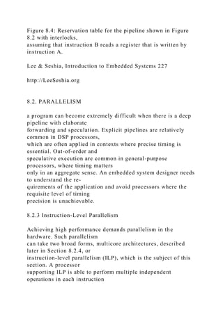
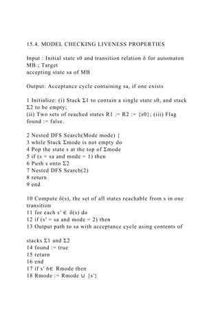
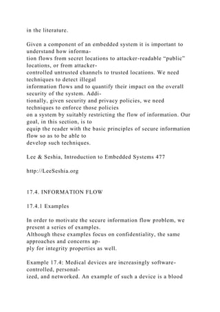
Compose Verify
Property
System
Environment
YES
[proof]
NO
counterexample
M
Figure 15.2: Formal verification procedure.
• The property to be verified Φ.
The verifier generates as output a YES/NO answer, indicating
whether or not S satisfies
the property Φ in environment E. Typically, a NO output is
accompanied by a counterex-
ample, also called an error trace, which is a trace of the system
that indicates how Φ is
violated. Counterexamples are very useful aids in the debugging
process. Some formal
verification tools also include a proof or certificate of
correctness with a YES answer;
such an output can be useful for certification of system
correctness.
The form of composition used to combine system model S with
environment model E

depends on the form of the interaction between system and
environment. Chapters 5
and 6 describe several ways to compose state machine models.
All of these forms of
composition can be used in generating a verification model M
from S and E. Note that
M can be nondeterministic.
For simplicity, in this chapter we will assume that system
composition has already been
performed using one of the techniques presented in Chapters 5
and 6. All algorithms
discussed in the following sections will operate on the
combined verification model M ,
and will be concerned with answering the question of whether
M satisfies property Φ.
Additionally, we will assume that Φ is specified as a property in
linear temporal logic.
15.2 Reachability Analysis
We consider first a special case of the model checking problem
which is useful in practice.
Specifically, we assume that M is a finite-state machine and Φ
is an LTL formula of the
form Gp, where p is a proposition. Recall from Chapter 13 that
Gp is the temporal logic
formula that holds in a trace when the proposition p holds in

every state of that trace. As
we have seen in Chapter 13, several system properties are
expressible as Gp properties.
We will begin in Section 15.2.1 by illustrating how computing
the reachable states of a
system enables one to verify a Gp property. In Section 15.2.2
we will describe a technique
for reachability analysis of finite-state machines based on
explicit enumeration of states.
Finally, in Section 15.2.3, we will describe an alternative
approach to analyze systems
with very large state spaces.
15.2.1 Verifying Gp
In order for a system M to satisfy Gp, where p is a proposition,
every trace exhibitable
by M must satisfy Gp. This property can be verified by
enumerating all states of M and
checking that every state satisfies p.
When M is finite-state, in theory, such enumeration is always
possible. As shown in
Chapter 3, the state space of M can be viewed as a directed
graph where the nodes of
the graph correspond to states of M and the edges correspond to
transitions of M . This
graph is called the state graph ofM , and the set of all states is
called its state space. With
this graph-theoretic viewpoint, one can see that checking Gp for
a finite-state system M
corresponds to traversing the state graph forM , starting from
the initial state and checking
that every state reached in this traversal satisfies p. Since M has
a finite number of states,

this traversal must terminate.
Example 15.1: Let the system S be the traffic light controller of
Figure 3.10 and
its environment E be the pedestrian model shown in Figure 3.11.
Let M be the
synchronous composition of S and E as shown in Figure 15.3.
Observe that M
is a closed system. Suppose that we wish to verify that M
satisfies the property
G ¬(green ∧ crossing)
In other words, we want to verify that it is never the case that
the traffic light is
green while pedestrians are crossing.
The composed system M is shown in Figure 15.4 as an extended
FSM. Note that
M has no inputs or outputs. M is finite-state, with a total of 188
states (using
a similar calculation to that in Example 3.12). The graph in
Figure 15.4 is not
Figure 15.3: Composition of traffic light controller (Figure
3.10) and pedestrian
model (Figure 3.11).
the full state graph of M , because each node represents a set of

states, one for
each different value of count in that node. However, through
visual inspection
of this graph we can check for ourselves that no state satisfies
the proposition
(green∧ crossing), and hence every trace satisfies the LTL
property G¬(green∧
crossing).
In practice, the seemingly simple task of verifying whether a
finite-state system M satis-
fies a Gp property is not as straightforward as in the previous
example for the following
reasons:
• Typically, one starts only with the initial state and transition
function, and the state
graph must be constructed on the fly.
Figure 15.4: Extended state machine obtained from
synchronous-reactive com-
position of traffic light controller and pedestrian models. Note
that this is nonde-
terministic.
• The system might have a huge number of states, possibly
exponential in the size of
the syntactic description of M . As a consequence, the state
graph cannot be repre-

sented using traditional data structures such as an adjacency or
incidence matrix.
The next two sections describe how these challenges can be
handled.
15.2.2 Explicit-State Model Checking
In this section, we discuss how to compute the reachable state
set by generating and
traversing the state graph on the fly.
First, recall that the system of interest M is closed, finite-state,
and can be nondetermin-
istic. Since M has no inputs, its set of possible next states is a
function of its current state
alone. We denote this transition relation ofM by δ, which is
only a function of the current
state of M , in contrast to the possibleUpdates function
introduced in Chapter 3 which is
also a function of the current input. Thus, δ(s) is the set of
possible next states from state
s of M .
Algorithm 15.1 computes the set of reachable states of M ,
given its initial state s0 and
transition relation δ. Procedure DFS Search performs a depth-
first traversal of the state

graph of M , starting with state s0. The graph is generated on-
the-fly by repeatedly apply-
ing δ to states visited during the traversal.
Input : Initial state s0 and transition relation δ for closed finite-
state
system M
Output: Set R of reachable states of M
1 Initialize: Stack Σ to contain a single state s0; Current set of
reached
states R := {s0}.
2 DFS Search() {
3 while Stack Σ is not empty do
4 Pop the state s at the top of Σ
5 Compute δ(s), the set of all states reachable from s in one
transition
6 for each s′ ∈ δ(s) do
7 if s′ 6∈ R then
8 R := R ∪ {s′}
9 Push s′ onto Σ
10 end
11 end
12 end
13 }
Algorithm 15.1: Computing the reachable state set by depth-
first explicit-state
search.
The main data structures required by the algorithm are Σ, the
stack storing the current

path in the state graph being explored from s0, and R, the
current set of states reached
during traversal. Since M is finite-state, at some point all states
reachable from s0 will
be in R, which implies that no new states will be pushed onto Σ
and thus Σ will become
empty. Hence, procedure DFS Search terminates and the value
of R at the end of the
procedure is the set of all reachable states of M .
The space and time requirements for this algorithm are linear in
the size of the state graph
(see Appendix B for an introduction to such complexity
notions). However, the number of
nodes and edges in the state graph of M can be exponential in
the size of the descriptions
of S and E. For example, if S and E together have 100 Boolean
state variables (a small
number in practice!), the state graph of M can have a total of
2100 states, far more than
what contemporary computers can store in main memory.
Therefore, explicit-state search
algorithms such as DFS Search must be augmented with state
compression techniques.
Some of these techniques are reviewed in the sidebar on page
424.
A challenge for model checking concurrent systems is the state-

explosion problem.
Recall that the state space of a composition of k finite-state
systems M1,M2, . . . ,Mk
(say, using synchronous composition), is the cartesian product
of the state spaces of
M1,M2, . . . ,Mk. In other words, if M1,M2, . . . ,Mk have n1,
n2, . . . , nk states respec-
tively, their composition can have Πki=1ni states. It is easy to
see that the number of states
of a concurrent composition of k components grows
exponentially with k. Explicitly rep-
resenting the state space of the composite system does not scale.
In the next section, we
will introduce techniques that can mitigate this problem in some
cases.
15.2.3 Symbolic Model Checking
The key idea in symbolic model checking is to represent a set of
states symbolically as
a propositional logic formula, rather than explicitly as a
collection of individual states.
Specialized data structures are often used to efficiently
represent and manipulate such
formulas. Thus, in contrast to explicit-state model checking, in
which individual states
are manipulated, symbolic model checking operates on sets of
states.
Algorithm 15.2 (Symbolic Search) is a symbolic algorithm for
computing the set of
reachable states of a closed, finite-state system M . This
algorithm has the same input-
output specification as the previous explicit-state algorithm
DFS Search; however, all
operations in Symbolic Search are set operations.

In algorithm Symbolic Search, R represents the entire set of
states reached at any point
in the search, and Rnew represents the new states generated at
that point. When no more
new states are generated, the algorithm terminates, with R
storing all states reachable
from s0. The key step of the algorithm is line 5, in which Rnew
is computed as the set
of all states s′ reachable from any state s in R in one step of the
transition relation δ.
This operation is called image computation, since it involves
computing the image of
the function δ. Efficient implementations of image computation
that directly operate on
propositional logic formulas are central to symbolic reachability
algorithms. Apart from
image computation, the key set operations in Symbolic Search
include set union and
emptiness checking.
Input : Initial state s0 and transition relation δ for closed finite-
state
system M , represented symbolically
Output: Set R of reachable states of M , represented
symbolically
1 Initialize: Current set of reached states R = {s0}

2 Symbolic Search() {
3 Rnew = R
4 while Rnew 6= ∅ do
5 Rnew := {s′ | ∃ s ∈ R s.t. s′ ∈ δ(s) ∧ s′ 6∈ R}
6 R := R ∪ Rnew
7 end
8 }
Algorithm 15.2: Computing the reachable state set by symbolic
search.
Example 15.2: We illustrate symbolic reachability analysis
using the finite-state
system in Figure 15.4.
To begin with, we need to introduce some notation. Let vl be a
variable denoting
the state of the traffic light controller FSM S at the start of each
reaction; i.e., vl ∈
{green, yellow, red, pending}. Similarly, let vp denote the state
of the pedestrian
FSM E, where vp ∈ {crossing, none,waiting}.
Given this notation, the initial state set {s0} of the composite
system M is repre-
sented as the following propositional logical formula:
vl = red ∧ vp = crossing ∧ count = 0
From s0, the only enabled outgoing transition is the self-loop on
the initial state
of the extended FSM in Figure 15.4. Thus, after one step of
reachability compu-
tation, the set of reached states R is represented by the
following formula:
vl = red ∧ vp = crossing ∧ 0 ≤ count ≤ 1

After two steps, R is given by
and after k steps, k ≤ 60, R is represented by the formula
vl = red ∧ vp = crossing ∧ 0 ≤ count ≤ k
On the 61st step, we exit the state (red, crossing), and compute
R as
∨ vl = green ∧ vp = none ∧ count = 0
Proceeding similarly, the set of reachable states R is grown
until there is no fur-
ther change. The final reachable set is represented as:
∨ vl = green ∧ vp = none ∧ 0 ≤ count ≤ 60
∨ vl = pending ∧ vp = waiting ∧ 0 < count ≤ 60
∨ vl = yellow ∧ vp = waiting ∧ 0 ≤ count ≤ 5
In practice, the symbolic representation is much more compact
than the explicit one. The
previous example illustrates this nicely because a large number
of states are compactly
represented by inequalities like 0 < count ≤ 60. Computer

programs can be designed
to operate directly on the symbolic representation. Some
examples of such programs are
given in the box on page 424.
Symbolic model checking has been used successfully to address
the state-explosion prob-
lem for many classes of systems, most notably for hardware
models. However, in the
worst case, even symbolic set representations can be
exponential in the number of system
variables.
15.3 Abstraction in Model Checking
A challenge in model checking is to work with the simplest
abstraction of a system that
will provide the required proofs of safety. Simpler abstractions
have smaller state spaces
and can be checked more efficiently. The challenge, of course,
is to know what details to
omit from the abstraction.
The part of the system to be abstracted away depends on the
property to be verified. The
following example illustrates this point.
15.3. ABSTRACTION IN MODEL CHECKING
Example 15.3: Consider the traffic light systemM in Figure
15.4. Suppose that,

as in Example 15.1 we wish to verify that M satisfies the
property
G ¬(green ∧ crossing)
Suppose we abstract the variable count away from M by hiding
all references to
count from the model, including all guards mentioning it and all
updates to it.
This generates the abstract model Mabs shown in Figure 15.5.
We observe that this abstract Mabs exhibits more behaviors than
M . For instance,
from the state (yellow,waiting) we can take the self-loop
transition forever, stay-
ing in that state perennially, even though in the actual system M
this state must
be exited within five clock ticks. Moreover, every behavior ofM
can be exhibited
by Mabs.
The interesting point is that, even with this approximation, we
can prove thatMabs
satisfies G ¬(green∧ crossing). The value of count is irrelevant
for this property.
Notice that while M has 188 states, Mabs has only 4 states.
Reachability analysis
on Mabs is far easier than for M as we have far fewer states to
explore.
There are several ways to compute an abstraction. One of the
simple and extremely
useful approaches is called localization reduction or localization
abstraction (Kurshan
(1994)). In localization reduction, parts of the design model that
are irrelevant to the

property being checked are abstracted away by hiding a subset
of state variables. Hiding
a variable corresponds to freeing that variable to evolve
arbitrarily. It is the form of
abstraction used in Example 15.3 above, where count is allowed
to change arbitrarily, and
all transitions are made independent of the value of count.
Example 15.4: Consider the multithreaded program given below
(adapted
from Ball et al. (2001)). The procedure lock unlock executes a
loop within
which it acquires a lock, then calls the function randomCall,
based on whose
result it either releases the lock and executes another loop
iteration, or it quits
the loop (and then releases the lock). The execution of another
loop iteration is
Figure 15.5: Abstraction of the traffic light system in Figure
15.4.
ensured by incrementing new, so that the condition old != new
evaluates to
true.
1 pthread_mutex_t lock = PTHREAD_MUTEX_INITIALIZER;
2 unsigned int old, new;
3

4 void lock_unlock() {
5 do {
6 pthread_mutex_lock(&lock);
7 old = new;
8 if (randomCall()) {
9 pthread_mutex_unlock(&lock);
10 new++;
11 }
12 } while (old != new)
14 }
Suppose the property we want to verify is that the code does not
attempt to call
pthread mutex lock twice in a row. Recall from Section 11.2.4
how the
system can deadlock if a thread becomes permanently blocked
trying to acquire a
lock. This could happen in the above example if the thread,
already holding lock
lock, attempts to acquire it again.
15.3. ABSTRACTION IN MODEL CHECKING
If we model this program exactly, without any abstraction, then
we need to reason
about all possible values of old and new, in addition to the
remaining state of the
program. Assuming a word size of 32 in this system, the size of

the state space is
roughly 232 × 232 × n, where 232 is the number of values of old
and new, and
n denotes the size of the remainder of the state space.
However, it is not necessary to reason about the precise values
of old and new
to prove that this program is correct. Assume, for this example,
that our pro-
gramming language is equipped with a boolean type. Assume
further that the
program can perform nondeterministic assignments. Then, we
can generate the
following abstraction of the original program, written in C-like
syntax, where the
Boolean variable b represents the predicate old == new.
1 pthread_mutex_t lock = PTHREAD_MUTEX_INITIALIZER;
2 boolean b; // b represents the predicate (old == new)
3 void lock_unlock() {
4 do {
5 pthread_mutex_lock(&lock);
6 b = true;
7 if (randomCall()) {
9 b = false;
10 }
11 } while (!b)
13 }
It is easy to see that this abstraction retains just enough
information to show that
the program satisfies the desired property. Specifically, the lock
will not be ac-

quired twice because the loop is only iterated if b is set to false,
which implies
that the lock was released before the next attempt to acquire.
Moreover, observe that size of the state space to be explored
has reduced to simply
2n. This is the power of using the “right” abstraction.
A major challenge for formal verification is to automatically
compute simple abstrac-
tions. An effective and widely-used technique is
counterexample-guided abstraction
refinement (CEGAR), first introduced by Clarke et al. (2000).
The basic idea (when
using localization reduction) is to start by hiding almost all
state variables except those
referenced by the temporal logic property. The resulting
abstract system will have more
behaviors than the original system. Therefore, if this abstract
system satisfies an LTL
formula Φ (i.e., each of its behaviors satisfies Φ), then so does
the original. However, if
the abstract system does not satisfy Φ, the model checker
generates a counterexample. If
this counterexample is a counterexample for the original
system, the process terminates,
having found a genuine counterexample. Otherwise, the CEGAR
approach analyzes this

counterexample to infer which hidden variables must be made
visible, and with these ad-
ditional variables, recomputes an abstraction. The process
continues, terminating either
with some abstract system being proven correct, or generating a
valid counterexample for
the original system.
The CEGAR approach and several follow-up ideas have been
instrumental in driving
progress in the area of software model checking. We review
some of the key ideas in the
sidebar on page 424.
15.4 Model Checking Liveness Properties
So far, we have restricted ourselves to verifying properties of
the form Gp, where p is an
atomic proposition. An assertion that Gp holds for all traces is a
very restricted kind of
safety property. However, as we have seen in Chapter 13,
several useful system properties
are not safety properties. For instance, the property stating that
“the robot must visit
location A” is a liveness property: if visiting location A is
represented by proposition q,
then this property is an assertion that Fq must hold for all
traces. In fact, several problems,
including path planning problems for robotics and progress
properties of distributed and
concurrent systems can be stated as liveness properties. It is
therefore useful to extend
model checking to handle this class of properties.
Properties of the form Fp, though liveness properties, can be
partially checked using the

techniques introduced earlier in this chapter. Recall from
Chapter 13 that Fp holds for
a trace if and only if ¬G¬p holds for the same trace. In words,
“p is true some time in
the future” iff “¬p is always false.” Therefore, we can attempt
to verify that the system
satisfies G¬p. If the verifier asserts that G¬p holds for all
traces, then we know that
Fp does not hold for any trace. On the other hand, if the verifier
outputs “NO”, then
the accompanying counterexample provides a witness exhibiting
how p may become true
eventually. This witness provides one trace for which Fp holds,
but it does not prove that
Fp holds for all traces (unless the machine is deterministic).
15.4. MODEL CHECKING LIVENESS PROPERTIES
More complete checks and more complicated liveness properties
require a more sophis-
ticated approach. Briefly, one approach used in explicit-state
model checking of LTL
properties is as follows:
1. Represent the negation of the property Φ as an automaton B,
where certain states
are labeled as accepting states.
2. Construct the synchronous composition of the property
automaton B and the sys-
tem automatonM . The accepting states of the property

automaton induce accepting
states of the product automaton MB .
3. If the product automaton MB can visit an accepting state
infinitely often, then it
indicates that M does not satisfy Φ; otherwise, M satisfies Φ.
The above approach is known as the automata-theoretic
approach to verification. We
give a brief introduction to this subject in the rest of this
section. Further details may be
found in the seminal papers on this topic (Wolper et al. (1983);
Vardi and Wolper (1986))
and the book on the SPIN model checker (Holzmann (2004)).
15.4.1 Properties as Automata
Consider the first step of viewing properties as automata. Recall
the material on omega-
regular languages introduced in the box on page 386. The theory
of Büchi automata and
omega-regular languages, briefly introduced there, is relevant
for model checking liveness
properties. Roughly speaking, an LTL property Φ has a one-to-
one correspondence with a
set of behaviors that satisfy Φ. This set of behaviors constitutes
the language of the Büchi
automaton corresponding to Φ.
For the LTL model checking approach we describe here, if Φ is
the property that the
system must satisfy, then we represent its negation ¬Φ as a
Büchi automaton. We present
some illustrative examples below.
Example 15.5: Suppose that an FSM M1 models a system that

executes forever
and produces a pure output h (for heartbeat), and that it is
required to produce this
output at least once every three reactions. That is, if in two
successive reactions
it fails to produce the output h, then in the third it must.
We can formulate this property in LTL as the property Φ1
below:
G(h ∨ Xh ∨ X2h)
and the negation of this property is
F(¬h ∧ X¬h ∧ X2¬h)
The Büchi automaton B1 corresponding to the negation of the
desired property is
given below:
Let us examine this automaton. The language accepted by this
automaton in-
cludes all behaviors that enter and stay in state d. Equivalently,
the language
includes all behaviors that produce a present output on f in
some reaction. When
we compose the above machine with M1, if the resulting
composite machine can
never produce f = present, then the language accepted by the

composite machine
is empty. If we can prove that the language is empty, then we
have proved that M
produces the heartbeat h at least once every three reactions.
Observe that the property Φ1 in the above example is in fact a
safety property. We give
an example of a liveness property below.
Example 15.6: Suppose that the FSM M2 models a controller for
a robot that
must locate a room and stay there forever. Let p be the
proposition that becomes
true when the robot is in the target room. Then, the desired
property Φ2 can be
expressed in LTL as FGp.
The negation of this property is GF¬p. The Büchi automaton B2
corresponding
to this negated property is given below:
Notice that all accepting behaviors of B2 correspond to those
where ¬p holds
infinitely often. These behaviors correspond to a cycle in the
state graph for the
product automaton where state b of B2 is visited repeatedly.
This cycle is known
as an acceptance cycle.

Liveness properties of the form GFp also occur naturally as
specifications. This form of
property is useful in stating fairness properties which assert that
certain desirable proper-
ties hold infinitely many times, as illustrated in the following
example.
Example 15.7: Consider a traffic light system such as that in
Example 3.10. We
may wish to assert that the traffic light becomes green infinitely
many times in
any execution. In other words, the state green is visited
infinitely often, which
can be expressed as Φ3 = GF green.
The automaton corresponding to Φ3 is identical to that for the
negation of Φ2
in Example 15.6 above with ¬p replaced by green. However, in
this case the
accepting behaviors of this automaton are the desired behaviors.
Thus, from these examples we see that the problem of detecting
whether a certain ac-
cepting state s in an FSM can be visited infinitely often is the
workhorse of explicit-state
model checking of LTL properties. We next present an
algorithm for this problem.
15.4.2 Finding Acceptance Cycles
We consider the following problem:

Given a finite-state system M , can an accepting state sa of M
be visited
infinitely often?
Put another way, we seek an algorithm to check whether (i)
state sa is reachable from
the initial state s0 of M , and (ii) sa is reachable from itself.
Note that asking whether a
state can be visited infinitely often is not the same as asking
whether it must be visited
infinitely often.
The graph-theoretic viewpoint is useful for this problem, as it
was in the case of Gp
discussed in Section 15.2.1. Assume for the sake of argument
that we have the entire state
graph constructed a priori. Then, the problem of checking
whether state sa is reachable
from s0 is simply a graph traversal problem, solvable for
example by depth-first search
(DFS). Further, the problem of detecting whether sa is reachable
from itself amounts to
checking whether there is a cycle in the state graph containing
that state.
The main challenges for solving this problem are similar to
those discussed in Sec-
tion 15.2.1: we must perform this search on-the-fly, and we
must deal with large state
spaces.
The nested depth-first search (nested DFS) algorithm, which is
implemented in the SPIN

model checker (Holzmann (2004)), solves this problem and is
shown as Algorithm 15.3.
The algorithm begins by calling the procedure called Nested
DFS Search with argument
1, as shown in the Main function at the bottom. MB is obtained
by composing the original
closed system M with the automaton B representing the
negation of LTL formula Φ.
As the name suggests, the idea is to perform two depth-first
searches, one nested inside the
other. The first DFS identifies a path from initial state s0 to the
target accepting state sa.
Then, from sa we start another DFS to see if we can reach sa
again. The variable mode
is either 1 or 2 depending on whether we are performing the
first DFS or the second.
Stacks Σ1 and Σ2 are used in the searches performed in modes 1
and 2 respectively. If
sa is encountered in the second DFS, the algorithm generates as
output the path leading
from s0 to sa with a loop on sa. The path from s0 to sa is
obtained simply by reading off
the contents of stack Σ1. Likewise, the cycle from sa to itself is
obtained from stack Σ2.
Otherwise, the algorithm reports failure.
Search optimization and state compression techniques that are
used in explicit-state reach-
ability analysis can be used with nested DFS also. Further
details are available in Holz-
mann (2004).

Input : Initial state s0 and transition relation δ for automaton
MB ; Target
accepting state sa of MB
Output: Acceptance cycle containing sa, if one exists
1 Initialize: (i) Stack Σ1 to contain a single state s0, and stack
Σ2 to be empty;
(ii) Two sets of reached states R1 := R2 := {s0}; (iii) Flag
found := false.
2 Nested DFS Search(Mode mode) {
3 while Stack Σmode is not empty do
4 Pop the state s at the top of Σmode
5 if (s = sa and mode = 1) then
6 Push s onto Σ2
7 Nested DFS Search(2)
8 return
9 end
10 Compute δ(s), the set of all states reachable from s in one
transition
11 for each s′ ∈ δ(s) do
12 if (s′ = sa and mode = 2) then
13 Output path to sa with acceptance cycle using contents of
stacks Σ1 and Σ2
14 found := true
15 return
16 end
17 if s′ 6∈ Rmode then
18 Rmode := Rmode ∪ {s′}

19 Push s′ onto Σmode
20 Nested DFS Search(mode)
21 end
22 end
23 end
24 }
25 Main() {
26 Nested DFS Search(1)
27 if (found = false) then Output “no acceptance cycle with sa”
end }
28
Algorithm 15.3: Nested depth-first search algorithm.
15.5 Summary
This chapter gives some basic algorithms for formal
verification, including model check-
ing, a technique for verifying if a finite-state system satisfies a
property specified in tem-
poral logic. Verification operates on closed systems, which are
obtained by composing a
system with its operating environment. The first key concept is
that of reachability anal-
ysis, which verifies properties of the form Gp. The concept of
abstraction, central to the
scalability of model checking, is also discussed in this chapter.
This chapter also shows
how explicit-state model checking algorithms can handle

liveness properties, where a cru-
cial concept is the correspondence between properties and
automata.
15.5. SUMMARY
Probing Further: Model Checking in Practice
Several tools are available for computing the set of reachable
states of a finite-state
system and checking that they satisfy specifications in temporal
logic. One such tool
is SMV (symbolic model verifier), which was first developed at
Carnegie Mellon Uni-
versity by Kenneth McMillan. SMV was the first model
checking tool to use binary
decision diagrams (BDDs), a compact data structure introduced
by Bryant (1986) for
representing a Boolean function. The use of BDDs has proved
instrumental in enabling
analysis of more complex systems. Current symbolic model
checkers also rely heav-
ily on Boolean satisfiability (SAT) solvers (see Malik and
Zhang (2009)), which are
programs for deciding whether a propositional logic formula can
evaluate to true. One
of the first uses of SAT solvers in model checking was for
bounded model checking
(see Biere et al. (1999)), where the transition relation of the
system is unrolled only a
bounded number of times. A few different versions of SMV are

available online (see
for example http://nusmv.fbk.eu/).
The SPIN model checker (Holzmann, 2004) developed in the
1980’s and 1990’s at
Bell Labs by Gerard Holzmann and others, is another leading
tool for model checking
(see http://www.spinroot.com/). Rather than directly
representing models as
communicating FSMs, it uses a specification language (called
Promela, for process
meta language) that enables specifications that closely resemble
multithreaded pro-
grams. SPIN incorporates state-compression techniques such as
hash compaction (the
use of hashing to reduce the size of the stored state set) and
partial-order reduction (a
technique to reduce the number of reachable states to be
explored by considering only
a subset of the possible process interleavings).
Automatic abstraction has played a big role in applying model
checking directly to
software. An example of abstraction-based software model
checking is the SLAM
system developed at Microsoft Research (Ball and Rajamani,
2001; Ball et al., 2011).
SLAM combines CEGAR with a particular form of abstraction
called predicate ab-
straction, in which predicates in a program are abstracted to
Boolean variables. A
key step in these techniques is checking whether a
counterexample generated on the
abstract model is in fact a true counterexample. This check is
performed using sat-
isfiability solvers for logics richer than propositional logic.

These solvers are called
SAT-based decision procedures or satisfiability modulo theories
(SMT) solvers (for
more details, see Barrett et al. (2009)).
More recently, techniques based on inductive learning, that is,
generalization from
sample data, have started playing an important role in formal
verification (see Seshia
(2015) for an exposition of this topic).
http://nusmv.fbk.eu/
http://www.spinroot.com/
Exercises
1. Consider the system M modeled by the hierarchical state
machine of Figure 13.2,
which models an interrupt-driven program.
Model M in the modeling language of a verification tool (such
as SPIN). You will
have to construct an environment model that asserts the
interrupt. Use the verifica-
tion tool to check whether M satisfies φ, the property stated in
Exercise 5:
φ: The main program eventually reaches program location C.
Explain the output you obtain from the verification tool.

2. Figure 15.3 shows the synchronous-reactive composition of
the traffic light con-
troller of Figure 3.10 and the pedestrian model of Figure 3.11.
Consider replacing the pedestrian model in Figure 15.3 with the
alternative model
given below where the initial state is nondeterministically
chosen to be one of none
or crossing:
(a) Model the composite system in the modeling language of a
verification tool
(such as SPIN). How many reachable states does the combined
system have?
How many of these are initial states?
(b) Formulate an LTL property stating that every time a
pedestrian arrives, even-
tually the pedestrian is allowed to cross (i.e., the traffic light
enters state red).
(c) Use the verification tool to check whether the model
constructed in part (a)
satisfies the LTL property specified in part (b). Explain the
output of the tool.
EXERCISES
3. The notion of reachability has a nice symmetry. Instead of
describing all states that

are reachable from some initial state, it is just as easy to
describe all states from
which some state can be reached. Given a finite-state system M
, the backward
reachable states of a set F of states is the set B of all states from
which some
state in F can be reached. The following algorithm computes the
set of backward
reachable states for a given set of states F :
Input : A set F of states and transition relation δ for closed
finite-state system M
Output: Set B of backward reachable states from F in M
1 Initialize: B := F
2 Bnew := B
3 while Bnew 6= ∅ do
4 Bnew := {s | ∃ s′ ∈ B s.t. s′ ∈ δ(s) ∧ s 6∈ B}
5 B := B ∪ Bnew
6 end
Explain how this algorithm can check the property Gp on M ,
where p is some
property that is easily checked for each state s in M . You may
assume that M has
exactly one initial state s0.
16
Quantitative Analysis

16.1 Problems of Interest . . . . . . . . . . . . . . . . . . . . . . . . . .
428
16.1.1 Extreme-Case Analysis . . . . . . . . . . . . . . . . . . . . . 429
16.1.2 Threshold Analysis . . . . . . . . . . . . . . . . . . . . . . . 429
16.1.3 Average-Case Analysis . . . . . . . . . . . . . . . . . . . . . 430
16.2 Programs as Graphs . . . . . . . . . . . . . . . . . . . . . . . . . . 430
16.2.1 Basic Blocks . . . . . . . . . . . . . . . . . . . . . . . . . . 431
16.2.2 Control-Flow Graphs . . . . . . . . . . . . . . . . . . . . . . 432
16.2.3 Function Calls . . . . . . . . . . . . . . . . . . . . . . . . . 432
16.3 Factors Determining Execution Time . . . . . . . . . . . . . . . .
435
16.3.1 Loop Bounds . . . . . . . . . . . . . . . . . . . . . . . . . . 436
16.3.2 Exponential Path Space . . . . . . . . . . . . . . . . . . . . . 438
16.3.3 Path Feasibility . . . . . . . . . . . . . . . . . . . . . . . . . 439
16.3.4 Memory Hierarchy . . . . . . . . . . . . . . . . . . . . . . . 440
16.4 Basics of Execution Time Analysis . . . . . . . . . . . . . . . . . .
442
16.4.1 Optimization Formulation . . . . . . . . . . . . . . . . . . . 442
16.4.2 Logical Flow Constraints . . . . . . . . . . . . . . . . . . . . 445
16.4.3 Bounds for Basic Blocks . . . . . . . . . . . . . . . . . . . . 449
16.5 Other Quantitative Analysis Problems . . . . . . . . . . . . . . .
. 451
16.5.1 Memory-bound Analysis . . . . . . . . . . . . . . . . . . . . 451
16.5.2 Power and Energy Analysis . . . . . . . . . . . . . . . . . . 452
16.6 Summary . . . . . . . . . . . . . . . . . . . . . . . . . . . . . . . . 452
Sidebar: Tools for Execution-Time Analysis . . . . . . . . . . . . . .
454
Exercises . . . . . . . . . . . . . . . . . . . . . . . . . . . . . . . . . . . 455

16.1. PROBLEMS OF INTEREST
Will my brake-by-wire system actuate the brakes within one
millisecond? Answering this
question requires, in part, an execution-time analysis of the
software that runs on the
electronic control unit (ECU) for the brake-by-wire system.
Execution time of the soft-
ware is an example of a quantitative property of an embedded
system. The constraint
that the system actuate the brakes within one millisecond is a
quantitative constraint.
The analysis of quantitative properties for conformance with
quantitative constraints is
central to the correctness of embedded systems and is the topic
of the present chapter.
A quantitative property of an embedded system is any property
that can be measured.
This includes physical parameters, such as position or velocity
of a vehicle controlled by
the embedded system, weight of the system, operating
temperature, power consumption,
or reaction time. Our focus in this chapter is on properties of
software-controlled sys-
tems, with particular attention to execution time. We present
program analysis techniques
that can ensure that execution time constraints will be met. We
also discuss how similar
techniques can be used to analyze other quantitative properties
of software, particularly
resource usage such as power, energy, and memory.
The analysis of quantitative properties requires adequate models
of both the software com-

ponents of the system and of the environment in which the
software executes. The envi-
ronment includes the processor, operating system, input-output
devices, physical compo-
nents with which the software interacts, and (if applicable) the
communication network.
The environment is sometimes also referred to as the platform
on which the software ex-
ecutes. Providing a comprehensive treatment of execution time
analysis would require
much more than one chapter. The goal of this chapter is more
modest. We illustrate
key features of programs and their environment that must be
considered in quantitative
analysis, and we describe qualitatively some analysis techniques
that are used. For con-
creteness, we focus on a single quantity, execution time, and
only briefly discuss other
resource-related quantitative properties.
16.1 Problems of Interest
The typical quantitative analysis problem involves a software
task defined by a program
P , the environment E in which the program executes, and the
quantity of interest q. We
assume that q can be given by a function of fP as follows,
q = fP (x,w)
16. QUANTITATIVE ANALYSIS

where x denotes the inputs to the program P (such as data read
from memory or from sen-
sors, or data received over a network), andw denotes the
environment parameters (such as
network delays or the contents of the cache when the program
begins executing). Defin-
ing the function fP completely is often neither feasible nor
necessary; instead, practical
quantitative analysis will yield extreme values for q (highest or
lowest values), average
values for q, or proofs that q satisfies certain threshold
constraints. We elaborate on these
next.
16.1.1 Extreme-Case Analysis
In extreme-case analysis, we may want to estimate the largest
value of q for all values of
x and w,
max
x,w
fP (x,w). (16.1)
Alternatively, it can be useful to estimate the smallest value of
q:
min
x,w
fP (x,w). (16.2)
If q represents execution time of a program or a program
fragment, then the largest value is

called the worst-case execution time (WCET), and the smallest
value is called the best-
case execution time (BCET). It may be difficult to determine
these numbers exactly, but
for many applications, an upper bound on the WCET or a lower
bound on the BCET is
all that is needed. In each case, when the computed bound
equals the actual WCET or
BCET, it is said to be a tight bound; otherwise, if there is a
considerable gap between the
actual value and the computed bound, it is said to be a loose
bound. Computing loose
bounds may be much easier than finding tight bounds.
16.1.2 Threshold Analysis
A threshold property asks whether the quantity q is always
bounded above or below by
a threshold T , for any choice of x and w. Formally, the
property can be expressed as
∀ x,w, fP (x,w) ≤ T (16.3)
or
∀ x,w, fP (x,w) ≥ T (16.4)
16.2. PROGRAMS AS GRAPHS
Threshold analysis may provide assurances that a quantitative
constraint is met, such as
the requirement that a brake-by-wire system actuate the brakes

within one millisecond.
Threshold analysis may be easier to perform than extreme-case
analysis. Unlike extreme-
case analysis, threshold analysis does not require us to
determine the maximum or mini-
mum value exactly, or even to find a tight bound on these
values. Instead, the analysis is
provided some guidance in the form of the target value T . Of
course, it might be possible
to use extreme-case analysis to check a threshold property.
Specifically, Constraint 16.3
holds if the WCET does not exceed T , and Constraint 16.4
holds if the BCET is not less
than T .
16.1.3 Average-Case Analysis
Often one is interested more in typical resource usage rather
than in worst-case scenarios.
This is formalized as average-case analysis. Here, the values of
input x and environment
parameter w are assumed to be drawn randomly from a space of
possible values X and
W according to probability distributions Dx and Dw
respectively. Formally, we seek to
estimate the value
EDx,DwfP (x,w) (16.5)
where EDx,Dw denotes the expected value of fP (x,w) over the
distributions Dx and Dw.
One difficulty in average-case analysis is to define realistic
distributions Dx and Dw that
capture the true distribution of inputs and environment

parameters with which a program
will execute.
In the rest of this chapter, we will focus on a single
representative problem, namely,
WCET estimation.
16.2 Programs as Graphs
A fundamental abstraction used often in program analysis is to
represent a program as a
graph indicating the flow of control from one code segment to
another. We will illustrate
this abstraction and other concepts in this chapter using the
following running example:
Example 16.1: Consider the function modexp that performs
modular expo-
nentiation, a key step in many cryptographic algorithms. In
modular exponen-
tiation, given a base b, an exponent e, and a modulus m, one
must compute
be mod m. In the program below, base, exponent and mod
represent b, e
and m respectively. EXP BITS denotes the number of bits in the
exponent. The
function uses a standard shift-square-accumulate algorithm,
where the base is
repeatedly squared, once for each bit position of the exponent,

and the base is
accumulated into the result only if the corresponding bit is set.
1 #define EXP_BITS 32
2
3 typedef unsigned int UI;
4
5 UI modexp(UI base, UI exponent, UI mod) {
6 int i;
7 UI result = 1;
8
9 i = EXP_BITS;
10 while(i > 0) {
11 if ((exponent & 1) == 1) {
12 result = (result * base) % mod;
13 }
14 exponent >>= 1;
15 base = (base * base) % mod;
16 i--;
17 }
18 return result;
19 }
16.2.1 Basic Blocks
A basic block is a sequence of consecutive program statements
in which the flow of
control enters only at the beginning of this sequence and leaves
only at the end, without
halting or the possibility of branching except at the end.

Example 16.2: The following three statements from the modexp
function in
Example 16.1 form a basic block:
14 exponent >>= 1;
16 i--;
Another example of a basic block includes the initializations at
the top of the
function, comprising lines 7 and 9:
7 result = 1;
8
9 i = EXP_BITS;
16.2.2 Control-Flow Graphs
A control-flow graph (CFG) of a program P is a directed graph
G = (V,E), where the
set of vertices V comprises basic blocks of P , and the set of
edges E indicates the flow
of control between basic blocks. Figure 16.1 depicts the CFG
for the modexp program
of Example 16.1. Each node of the CFG is labeled with its
corresponding basic block. In
most cases, this is simply the code as it appears in Example
16.1. The only exception is
for conditional statements, such as the conditions in while loops
and if statements; in

these cases, we follow the convention of labeling the node with
the condition followed by
a question mark to indicate the conditional branch.
Although our illustrative example of a control-flow graph is at
the level of C source code,
it is possible to use the CFG representation at other levels of
program representation
as well, including a high-level model as well as low-level
assembly code. The level of
representation employed depends on the level of detail required
by the context. To make
them easier to follow, our control-flow graphs will be at the
level of source code.
16.2.3 Function Calls
Programs are typically decomposed into several functions in
order to systematically or-
ganize the code and promote reuse and readability. The control-
flow graph (CFG) repre-
sentation can be extended to reason about code with function
calls by introducing special
call and return edges. These edges connect the CFG of the caller
function – the one
making the function call – to that of the callee function – the
one being called. A call
edge indicates a transfer of control from the caller to the callee.

A return edge indicates
a transfer of control from the callee back to the caller.
result = 1;
i = EXP_BITS;
(i > 0)?
((exponent & 1) == 1)?
result = (result * base) % mod;
exponent >>= 1;
base = (base * base) % mod;
i--;
return result;
1
0
1
0
1
2
3
4

5
6
Figure 16.1: Control-flow graph for the modexp function of
Example 16.1. All
incoming edges at a node indicate transfer of control to the start
of the basic
block for that node, and all outgoing edges from a node indicate
an exit from the
end of the basic block for that node. For clarity, we label the
outgoing edges from
a branch statement with 0 or 1 indicating the flow of control in
case the branch
evaluates to false or true, respectively. An ID number for each
basic block is noted
above the node for that block; IDs range from 1 to 6 for this
example.
result = 1;
i = EXP_BITS;
(i > 0)?
result = update(result);
i--;

return result;
1
0
res = r;
((exponent & 1) == 1)?
res = (res * base) % mod;
exponent >>= 1;
base = (base * base) % mod;
0
1
return res;
call
return
Figure 16.2: Control-flow graphs for the modexp call and
update functions in
Example 16.3. Call/return edges are indicated with dashed lines.
Example 16.3: A slight variant shown below of the modular
exponentation
program of Example 16.1 uses function calls and can be
represented by the CFG
with call and return edges in Figure 16.2.

3 UI exponent, base, mod;
4
5 UI update(UI r) {
6 UI res = r;
7 if ((exponent & 1) == 1) {
8 res = (res * base) % mod;
9 }
10 exponent >>= 1;
12 return res;
13 }
14
15 UI modexp_call() {
16 UI result = 1; int i;
17 i = EXP_BITS;
18 while(i > 0) {
19 result = update(result);
20 i--;
21 }
22 return result;
23 }
In this modified example, the variables base, exponent, and mod

are global
variables. The update to base and exponent in the body of the
while loop,
along with the computation of result is now performed in a
separate function
named update.
Non-recursive function calls can also be handled by inlining,
which is the process of
copying the code for the callee into that of the caller. If inlining
is performed transitively
for all functions called by the code that must be analyzed, the
analysis can be performed
on the CFG of the code resulting from inlining, without using
call and return edges.
16.3 Factors Determining Execution Time
There are several issues one must consider in order to estimate
the worst-case execution
time of a program. This section outlines some of the main issues
and illustrates them with
examples. In describing these issues, we take a programmer’s
viewpoint, starting with the
program structure and then considering how the environment
can impact the program’s
execution time.
16.3. FACTORS DETERMINING EXECUTION TIME
16.3.1 Loop Bounds

The first point one must consider when bounding the execution
time of a program is
whether the program terminates. Non-termination of a
sequential program can arise from
non-terminating loops or from an unbounded sequence of
function calls. Therefore, while
writing real-time embedded software, the programmer must
ensure that all loops are guar-
anteed to terminate. In order to guarantee this, one must
determine for each loop a bound
on the number of times that loop will execute in the worst case.
Similarly, all function
calls must have bounded recursion depth. The problems of
determining bounds on loop
iterations or recursion depth are undecidable in general, since
the halting problem for Tur-
ing machines can be reduced to either problem. (See Appendix
B for an introduction to
Turing machines and decidability.)
In this section, we limit ourselves to reasoning about loops. In
spite of the undeciable
nature of the problem, progress has been made on automatically
determining loop bounds
for several patterns that arise in practice. Techniques for
determining loop bounds are a
current research topic and a full survey of these methods is out
of the scope of this chapter.
We will limit ourselves to presenting illustrative examples for
loop bound inference.
The simplest case is that of for loops that have a specified
constant bound, as in Exam-
ple 16.4 below. This case occurs often in embedded software, in
part due to a discipline

of programming enforced by designers who must program for
real-time constraints and
limited resources.
Example 16.4: Consider the function modexp1 below. It is a
slight variant of
the function modexp introduced in Example 16.1 that performs
modular expo-
nentiation, in which the while loop has been expressed as an
equivalent for
loop.
2
4
5 UI modexp1(UI base, UI exponent, UI mod) {
6 UI result = 1; int i;
7
8 for(i=EXP_BITS; i > 0; i--) {
9 if ((exponent & 1) == 1) {
11 }
12 exponent >>= 1;

14 }
15 return result;
16 }
In the case of this function, it is easy to see that the for loop
will take exactly
EXP BITS iterations, where EXP BITS is defined as the
constant 32.
In many cases, the loop bound is not immediately obvious (as it
was for the above exam-
ple). To make this point, here is a variation on Example 16.4.
Example 16.5: The function listed below also performs modular
exponentiation,
as in Example 16.4. However, in this case, the for loop is
replaced by a while
loop with a different loop condition – the loop exits when the
value of exponent
reaches 0. Take a moment to check whether the while loop will
terminate (and
if so, why).
2
3 UI modexp2(UI base, UI exponent, UI mod) {
4 UI result = 1;
5
6 while (exponent != 0) {
7 if ((exponent & 1) == 1) {
9 }

10 exponent >>= 1;
12 }
13 return result;
14 }
Now let us analyze the reason that this loop terminates. Notice
that exponent
is an unsigned int, which we will assume to be 32 bits wide. If
it starts out equal
to 0, the loop terminates right away and the function returns
result = 1. If
not, in each iteration of the loop, notice that line 10 shifts
exponent one bit
to the right. Since exponent is an unsigned int, after the right
shift, its most
significant bit will be 0. Reasoning thus, after at most 32 right
shifts, all bits of
exponent must be set to 0, thus causing the loop to terminate.
Therefore, we
can conclude that the loop bound is 32.
Let us reflect on the reasoning employed in the above example.
The key component of
our “proof of termination” was the observation that the number
of bits of exponent
decreases by 1 each time the loop executes. This is a standard
argument for proving

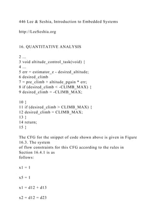
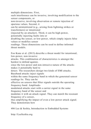
termination – by defining a progress measure or ranking
function that maps each state
of the program to a mathematical structure called a well order.
Intuitively, a well order is
like a program that counts down to zero from some initial value
in the natural numbers.
16.3.2 Exponential Path Space
Execution time is a path property. In other words, the amount of
time taken by the pro-
gram is a function of how conditional statements in the program
evaluate to true or false.
A major source of complexity in execution time analysis (and
other program analysis
problems as well) is that the number of program paths can be
very large — exponential in
the size of the program. We illustrate this point with the
example below.
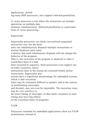
Example 16.6: Consider the function count listed below, which
runs over
a two-dimensional array, counting and accumulating non-
negative and negative
elements of the array separately.
1 #define MAXSIZE 100
2
3 int Array[MAXSIZE][MAXSIZE];
4 int Ptotal, Pcnt, Ntotal, Ncnt;
5 ...
6 void count() {
7 int Outer, Inner;
8 for (Outer = 0; Outer < MAXSIZE; Outer++) {
9 for (Inner = 0; Inner < MAXSIZE; Inner++) {

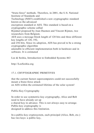
10 if (Array[Outer][Inner] >= 0) {
11 Ptotal += Array[Outer][Inner];
12 Pcnt++;
13 } else {
14 Ntotal += Array[Outer][Inner];
15 Ncnt++;
16 }
17 }
18 }
19 }
The function includes a nested loop. Each loop executes
MAXSIZE (100) times.
Thus, the inner body of the loop (comprising lines 10–16) will
execute 10,000
times – as many times as the number of elements of Array. In
each iteration of
the inner body of the loop, the conditional on line 10 can either
evaluate to true or
false, thus resulting in 210000 possible ways the loop can
execute. In other words,
this program has 210000 paths.
Fortunately, as we will see in Section 16.4.1, one does not need
to explicitly enumerate
all possible program paths in order to perform execution time
analysis.

16.3.3 Path Feasibility
Another source of complexity in program analysis is that all
program paths may not be
executable. A computationally expensive function is irrelevant
for execution time analysis
if that function is never executed.
A path p in program P is said to be feasible if there exists an
input x to P such that
P executes p on x. In general, even if P is known to terminate,
determining whether a
path p is feasible is a computationally intractable problem. One
can encode the canonical
NP-complete problem, the Boolean satisfiability problem (see
Appendix B), as a problem
of checking path feasibility in a specially-constructed program.
In practice, however, in
many cases, it is possible to determine path feasibility.
Example 16.7: Recall Example 13.3 of a software task from the
open source
Paparazzi unmanned aerial vehicle (UAV) project (Nemer et al.,
2006):
1 #define PPRZ_MODE_AUTO2 2
2 #define PPRZ_MODE_HOME 3
3 #define VERTICAL_MODE_AUTO_ALT 3

4 #define CLIMB_MAX 1.0
5 ...
7 if (pprz_mode == PPRZ_MODE_AUTO2
8 || pprz_mode == PPRZ_MODE_HOME) {
9 if (vertical_mode == VERTICAL_MODE_AUTO_ALT) {
10 float err = estimator_z - desired_altitude;
11 desired_climb
15 }
18 }
19 }
20 }
21 }
This program has 11 paths in all. However, the number of
feasible program
paths is only 9. To see this, note that the two conditionals
desired climb
< -CLIMB MAX on line 13 and desired climb > CLIMB MAX
on line 16
cannot both be true. Thus, only three out of the four paths
through the two inner-
most conditional statements are feasible. This infeasible inner
path can be taken
for two possible evaluations of the outermost conditional on
lines 7 and 8: either
if pprz mode == PPRZ MODE AUTO2 is true, or if that
condition is false, but
pprz mode == PPRZ MODE HOME is true.

16.3.4 Memory Hierarchy
The preceding sections have focused on properties of programs
that affect execution time.
We now discuss how properties of the execution platform,
specifically of cache memories,
can significantly impact execution time. We illustrate this point
using Example 16.8.1 The
material on caches introduced in Sec. 9.2.3 is pertinent to this
discussion.
1This example is based on a similar example in Bryant and
O’Hallaron (2003).
Example 16.8: Consider the function dot product listed below,
which
computes the dot product of two vectors of floating point
numbers. Each vector
is of dimension n, where n is an input to the function. The
number of iterations
of the loop depends on the value of n. However, even if we
know an upper bound
on n, hardware effects can still cause execution time to vary
widely for similar
values of n.
1 float dot_product(float *x, float *y, int n) {
2 float result = 0.0;
3 int i;

4 for(i=0; i < n; i++) {
5 result += x[i] * y[i];
6 }
7 return result;
8 }
Suppose this program is executing on a 32-bit processor with a
direct-mapped
cache. Suppose also that the cache can hold two sets, each of
which can hold 4
floats. Finally, let us suppose that x and y are stored
contiguously in memory
starting with address 0.
Let us first consider what happens if n = 2. In this case, the
entire arrays x and
y will be in the same block and thus in the same cache set.
Thus, in the very
first iteration of the loop, the first access to read x[0] will be a
cache miss, but
thereafter every read to x[i] and y[i] will be a cache hit,
yielding best case
performance for loads.
Consider next what happens when n = 8. In this case, each x[i]
and y[i] map
to the same cache set. Thus, not only will the first access to
x[0] be a miss, the
first access to y[0] will also be a miss. Moreover, the latter
access will evict
the block containing x[0]-x[3], leading to a cache miss on x[1],
x[2], and
x[3] as well. The reader can see that every access to an x[i] or
y[i] will
lead to a cache miss.

Thus, a seemingly small change in the value of n from 2 to 8
can lead to a drastic
change in execution time of this function.
16.4. BASICS OF EXECUTION TIME ANALYSIS
16.4 Basics of Execution Time Analysis
Execution time analysis is a current research topic, with many
problems still to be solved.
There have been over two decades of research, resulting in a
vast literature. We cannot
provide a comprehensive survey of the methods in this chapter.
Instead, we will present
some of the basic concepts that find widespread use in current
techniques and tools for
WCET analysis. Readers interested in a more detailed treatment
may find an overview
in a recent survey paper (Wilhelm et al., 2008) and further
details in books (e.g., Li and
Malik (1999)) and book chapters (e.g., Wilhelm (2005)).
16.4.1 Optimization Formulation
An intuitive formulation of the WCET problem can be
constructed using the view of
programs as graphs. Given a program P , let G = (V,E) denote
its control-flow graph
(CFG). Let n = |V | be the number of nodes (basic blocks) in G,
and m = |E| denote the
number of edges. We refer to the basic blocks by their index i,

where i ranges from 1 to
n.
We assume that the CFG has a unique start or source node s and
a unique sink or end
node t. This assumption is not restrictive: If there are multiple
start or end nodes, one
can add a dummy start/end node to achieve this condition.
Usually we will set s = 1 and
t = n.
Let xi denote the number of times basic block i is executed. We
call xi the execution
count of basic block i. Let x = (x1, x2, . . . , xn) be a vector of
variables recording
execution counts. Not all valuations of x correspond to valid
program executions. We say
that x is valid if the elements of x correspond to a (valid)
execution of the program. The
following example illustrates this point.
Example 16.9: Consider the CFG for the modular
exponentiation function
modexp introduced in Example 16.1. There are six basic blocks
in this func-
tion, labeled 1 to 6 in Figure 16.1. Thus, x = (x1, x2, . . . , x6).
Basic blocks 1
and 6, the start and end, are each executed only once. Thus, x1
= x6 = 1; any
other valuation cannot correspond to any program execution.

Next consider basic blocks 2 and 3, corresponding to the
conditional branches
i > 0 and (exponent & 1) == 1. One can observe that x2 must
equal
x3 + 1, since the block 3 is executed every time block 2 is
executed, except when
the loop exits to block 6.
Along similar lines, one can see that basic blocks 3 and 5 must
be executed an
equal number of times.
Flow Constraints
The intuition expressed in Example 16.9 can be formalized
using the theory of network
flow, which finds use in many contexts including modeling
traffic, fluid flow, and the flow
of current in an electrical circuit. In particular, in our problem
context, the flow must
satisfy the following two properties:
1. Unit Flow at Source: The control flow from source node s = 1
to sink node t = n
is a single execution and hence corresponds to unit flow from
source to sink. This
property is captured by the following two constraints:
x1 = 1 (16.6)
xn = 1 (16.7)
2. Conservation of Flow: For each node (basic block) i, the
incoming flow to i from

its predecessor nodes equals the outgoing flow from i to its
successor nodes.
To capture this property, we introduce additional variables to
record the number
of times that each edge in the CFG is executed. Following the
notation of Li and
Malik (1999), let dij denote the number of times the edge from
node i to node j in
the CFG is executed. Then we require that for each node i, 1 ≤ i
≤ n,
xi =
∑
j∈ Pi
dji =
∑
j∈ Si
dij , (16.8)
where Pi is the set of predecessors to node i and Si is the set of
successors. For the
source node, P1 = ∅ , so the sum over predecessor nodes is
omitted. Similarly, for
the sink node, Sn = ∅ , so the sum over successor nodes is
omitted.

Taken together, the two sets of constraints presented above
suffice to implicitly define all
source-to-sink execution paths of the program. Since this
constraint-based representation
is an implicit representation of program paths, this approach is
also referred to in the
literature as implicit path enumeration or IPET.
We illustrate the generation of the above constraints with an
example.
Example 16.10: Consider again the function modexp of Example
16.1, with
CFG depicted in Figure 16.1.
The constraints for this CFG are as follows:
x1 = 1
x6 = 1
x1 = d12
x2 = d12 + d52 = d23 + d26
x3 = d23 = d34 + d35
x4 = d34 = d45
x5 = d35 + d45 = d52
x6 = d26
Any solution to the above system of equations will result in
integer values for
the xi and dij variables. Furthermore, this solution will generate

valid execution
counts for basic blocks. For example, one such valid solution is
x1 = 1, d12 = 1, x2 = 2, d23 = 1, x3 = 1, d34 = 0, d35 = 1,
x4 = 0, d45 = 0, x5 = 1, d52 = 1, x6 = 1, d26 = 1.
Readers are invited to find and examine additional solutions for
themselves.
Overall Optimization Problem
We are now in a position to formulate the overall optimization
problem to determine
worst-case execution time. The key assumption we make in this
section is that we know
an upper bound wi on the execution time of the basic block i.
(We will later see in
Section 16.4.3 how the execution time of a single basic block
can be bounded.) Then the
WCET is given by the maximum
∑n
i=1wixi over valid execution counts xi.
Putting this together with the constraint formulation of the
preceding section, our goal is
to find values for xi that give

max
xi, 1≤i≤n
n∑
i=1
wixi
subject to
x1 = xn = 1
xi =
∑
j∈ Pi
dji =
∑
j∈ Si
dij
This optimization problem is a form of a linear programming
(LP) problem (also called
a linear program), and it is solvable in polynomial time.
However, two major challenges remain:
• This formulation assumes that all source to sink paths in the
CFG are feasible and
does not bound loops in paths. As we have already seen in
Section 16.3, this is
not the case in general, so solving the above maximization
problem may yield a
pessimistic loose bound on the WCET. We will consider this

challenge in Sec-
tion 16.4.2.
• The upper bounds wi on execution time of basic blocks i are
still to be determined.
We will briefly review this topic in Section 16.4.3.
16.4.2 Logical Flow Constraints
In order to ensure that the WCET optimization is not too
pessimistic by including paths
that cannot be executed, we must add so-called logical flow
constraints. These con-
straints rule out infeasible paths and incorporate bounds on the
number of loop iterations.
We illustrate the use of such constraints with two examples.
Loop Bounds
For programs with loops, it is necessary to use bounds on loop
iterations to bound execu-
tion counts of basic blocks.
Example 16.11: Consider the modular exponentiation program
of Example 16.1
for which we wrote down flow constraints in Example 16.10.
Notice that those constraints impose no upper bound on x2 or
x3. As argued

in Examples 16.4 and 16.5, the bound on the number of loop
iterations in this
example is 32. However, without imposing this additional
constraint, since there
is no upper bound on x2 or x3, the solution to our WCET
optimization will be
infinite, implying that there is no upper bound on the WCET.
The following single
constraint suffices:
x3 ≤ 32
From this constraint on x3, we derive the constraint that x2 ≤
33, and also upper
bounds on x4 and x5. The resulting optimization problem will
then return a finite
solution, for finite values of wi.
Adding such bounds on values of xi does not change the
complexity of the optimization
problem. It is still a linear programming problem.
Infeasible Paths
Some logical flow constraints rule out combinations of basic
blocks that cannot appear
together on a single path.
Example 16.12: Consider a snippet of code from Example 16.7
describing a
software task from the open source Paparazzi unmanned aerial
vehicle (UAV)
project (Nemer et al., 2006):
1 #define CLIMB_MAX 1.0

2 ...
4 ...
5 err = estimator_z - desired_altitude;
6 desired_climb
10 }
13 }
14 return;
15 }
The CFG for the snippet of code shown above is given in Figure
16.3. The system
of flow constraints for this CFG according to the rules in
Section 16.4.1 is as
follows:
x1 = 1
x5 = 1
x1 = d12 + d13
x2 = d12 = d23

x3 = d13 + d23 = d34 + d35
x4 = d34 = d45
x5 = d35 + d45
A solution for the above system of equations is
x1 = x2 = x3 = x4 = x5 = 1,
implying that each basic block gets executed exactly once, and
that both condi-
tionals evaluate to true. However, as we discussed in Example
16.7, it is im-
possible for both conditionals to evaluate to true. Since CLIMB
MAX = 1.0, if
desired climb is less than −1.0 in basic block 1, then at the start
of basic
block 3 it will be set to −1.0.
The following constraint rules out the infeasible path:
d12 + d34 ≤ 1 (16.9)
err = estimator_z - desired_altitude;
desired_climb
= pre_climb + altitude_pgain * err;

(desired_climb < -CLIMB_MAX)?
desired_climb = -CLIMB_MAX;
(desired_climb > CLIMB_MAX)?
return;
1
0
0
1
2
3
4
5
desired_climb = CLIMB_MAX;
1
Figure 16.3: Control-flow graph for Example 16.12.
This constraint specifies that both conditional statements cannot
be true together.
It is of course possible for both conditionals to be false. We can
check that this
constraint excludes the infeasible path when added to the

original system.
More formally, for a program without loops, if a set of k edges
(i1, j1), (i2, j2), . . . , (ik, jk)
in the CFG cannot be taken together in a program execution, the
following constraint is
added to the optimization problem:
di1j1 + di2j2 + . . .+ dikjk ≤ k − 1 (16.10)
For programs with loops, the constraint is more complicated
since an edge can be tra-
versed multiple times, so the value of a dij variable can exceed
1. We omit the details in
this case; the reader can consult Li and Malik (1999) for a more
elaborate discussion of
this topic.
In general, the constraints added above to exclude infeasible
combinations of edges can
change the complexity of the optimization problem, since one
must also add the following
integrality constraints:
xi ∈ N, for all i = 1, 2, . . . , n (16.11)
dij ∈ N, for all i, j = 1, 2, . . . , n (16.12)

In the absence of such integrality constraints, the optimization
solver can return fractional
values for the xi and dij variables. However, adding these
constraints results in an inte-
ger linear programming (ILP) problem. The ILP problem is
known to be NP-hard (see
Appendix B, Section B.4). Even so, in many practical instances,
one can solve these ILP
problems fairly efficiently (see for example Li and Malik
(1999)).
16.4.3 Bounds for Basic Blocks
In order to complete the optimization problem for WCET
analysis, we need to compute
upper bounds on the execution times of basic blocks – the wi
coefficients in the cost func-
tion of Section 16.4.1. Execution time is typically measured in
CPU cycles. Generating
such bounds requires detailed microarchitectural modeling. We
briefly outline some of
the issues in this section.
A simplistic approach to this problem would be to generate
conservative upper bounds
on the execution time of each instruction in the basic block, and
then add up these per-
instruction bounds to obtain an upper bound on the execution
time of the overall basic
block.
The problem with this approach is that there can be very wide
variation in the execution
times for some instructions, resulting in very loose upper
bounds on the execution time

of a basic block. For instance, consider the latency of memory
instructions (loads and
stores) for a system with a data cache. The difference between
the latency when there
is a cache miss versus a hit can be a factor of 100 on some
platforms. In these cases,
if the analysis does not differentiate between cache hits and
misses, it is possible for the
computed bound to be a hundred times larger than the execution
time actually exhibited.
Several techniques have been proposed to better use program
context to predict execution
time of instructions more precisely. These techniques involve
detailed microarchitectural
modeling. We mention two main approaches below:
• Integer linear programming (ILP) methods: In this approach,
pioneered by Li and
Malik (1999), one adds cache constraints to the ILP formulation
of Section 16.4.1.
Cache constraints are linear expressions used to bound the
number of cache hits and
misses within basic blocks. The approach tracks the memory
locations that cause
cache conflicts – those that map onto the same cache set, but
have different tags –
and adds linear constraints to record the impact of such
conflicts on the number of

cache hits and misses. Measurement through simulation or
execution on the actual
platform must be performed to obtain the cycle count for hits
and misses. The cost
constraint of the ILP is modified to compute the program path
along which the
overall number of cycles, including cache hits and misses, is the
largest. Further
details about this approach are available in Li and Malik (1999).
• Abstract interpretation methods: Abstract interpretation is a
theory of approx-
imation of mathematical structures, in particular those that arise
in defining the
semantic models of computer systems (Cousot and Cousot
(1977)). In particular,
in abstract interpretation, one performs sound approximation,
where the set of
behaviors of the system is a subset of that of the model
generated by abstract inter-
pretation. In the context of WCET analysis, abstract
interpretation has been used
to infer invariants at program points, in order to generate loop
bounds, and con-
straints on the state of processor pipelines or caches at the entry
and exit locations
of basic blocks. For example, such a constraint could specify
the conditions under
which variables will be available in the data cache (and hence a
cache hit will re-
sult). Once such constraints are generated, one can run
measurements from states
satisfying those constraints in order to generate execution time
estimates. Further
details about this approach can be found in Wilhelm (2005).

In addition to techniques such as those described above,
accurate measurement of execu-
tion time is critical for finding tight WCET bounds. Some of the
measurement techniques
are as follows:
1. Sampling CPU cycle counter: Certain processors include a
register that records the
number of CPU cycles elapsed since reset. For example, the
time stamp counter
register on x86 architectures performs this function, and is
accessible through a
rdtsc (“read time stamp counter”) instruction. However, with
the advent of multi-
core designs and power management features, care must be
taken to use such CPU
cycle counters to accurately measure timing. For example, it
may be necessary to
lock the process to a particular CPU.
2. Using a logic analyzer: A logic analyzer is an electronic
instrument used to mea-
sure signals and track events in a digital system. In the current
context, the events of
interest are the entry and exit points of the code to be timed,
definable, for example,
as valuations of the program counter. Logic analyzers are less
intrusive than using

cycle counters, since they do not require instrumenting the
code, and they can be
more accurate. However, the measurement setup is more
complicated.
3. Using a cycle-accurate simulator: In many cases, timing
analysis must be per-
formed when the actual hardware is not yet available. In this
situation, a cycle-
accurate simulator of the platform provides a good alternative.
16.5 Other Quantitative Analysis Problems
Although we have focused mainly on execution time in this
chapter, several other quan-
titative analysis problems are relevant for embedded systems.
We briefly describe two of
these in this section.
16.5.1 Memory-bound Analysis
Embedded computing platforms have very limited memory as
compared to general-purpose
computers. For example, as mentioned in Chapter 9, the
Luminary Micro LM3S8962 con-
troller has only 64 KB of RAM. It is therefore essential to
structure the program so that
it uses memory efficiently. Tools that analyze memory
consumption and compute bounds
on memory usage can be very useful.
There are two kinds of memory bound analysis that are relevant
for embedded systems.
In stack size analysis (or simply stack analysis), one needs to
compute an upper bound
on the amount of stack-allocated memory used by a program.

Recall from Section 9.3.2
that stack memory is allocated whenever a function is called or
an interrupt is handled. If
the program exceeds the memory allocated for the stack, a stack
overflow is said to occur.
16.6. SUMMARY
If the program does not contain recursive functions and runs
uninterrupted, one can bound
stack usage by traversing the call graph of the program – the
graph that tracks which
functions call which others. If the space for each stack frame is
known, then one can track
the sequence of calls and returns along paths in the call graph in
order to compute the
worst-case stack size.
Performing stack size analysis for interrupt-driven software is
significantly more compli-
cated. We point the interested reader to Brylow et al. (2001).
Heap analysis is the other memory bound analysis problem that
is relevant for embedded
systems. This problem is harder than stack bound analysis since
the amount of heap space
used by a function might depend on the values of input data and
may not be known prior
to run-time. Moreover, the exact amount of heap space used by
a program can depend on
the implementation of dynamic memory allocation and the

garbage collector.
16.5.2 Power and Energy Analysis
Power and energy consumption are increasingly important
factors in embedded system
design. Many embedded systems are autonomous and limited by
battery power, so a
designer must ensure that the task can be completed within a
limited energy budget. Also,
the increasing ubiquity of embedded computing is increasing its
energy footprint, which
must be reduced for sustainable development.
To first order, the energy consumed by a program running on an
embedded device depends
on its execution time. However, estimating execution time alone
is not sufficient. For
example, energy consumption depends on circuit switching
activity, which can depend
more strongly on the data values with which instructions are
executed.
For this reason, most techniques for energy and power
estimation of embedded soft-
ware focus on estimating the average-case consumption. The
average case is typically
estimated by profiling instructions for several different data
values, guided by software
benchmarks. For an introduction to this topic, see Tiwari et al.
(1994).
16.6 Summary
Quantitative properties, involving physical parameters or
specifying resource constraints,

are central to embedded systems. This chapter gave an
introduction to basic concepts in
quantitative analysis. First, we considered various types of
quantitative analysis problems,
including extreme-case analysis, average-case analysis, and
verifying threshold proper-
ties. As a representative example, this chapter focused on
execution time analysis. Sev-
eral examples were presented to illustrate the main issues,
including loop bounds, path
feasibility, path explosion, and cache effects. An optimization
formulation that forms the
backbone of execution time analysis was presented. Finally, we
briefly discussed two
other quantitative analysis problems, including computing
bounds on memory usage and
on power or energy consumption.
Quantitative analysis remains an active field of research –
exemplifying the challenges in
bridging the cyber and physical aspects of embedded systems.
16.6. SUMMARY

Tools for Execution-Time Analysis
Current techniques for execution-time analysis are broadly
classified into those primar-
ily based on static analysis and those that are measurement-
based.
Static tools rely on abstract interpretation and dataflow analysis
to compute facts
about the program at selected program locations. These facts are
used to identify de-
pendencies between code fragments, generate loop bounds, and
identify facts about the
platform state, such as the state of the cache. These facts are
used to guide timing mea-
surements of basic blocks and combined into an optimization
problem as presented
in this chapter. Static tools aim to find conservative bounds on
extreme-case execu-
tion time; however, they are not easy to port to new platforms,
often requiring several
man-months of effort.
Measurement-based tools are primarily based on testing the
program on multiple
inputs and then estimating the quantity of interest (e.g., WCET)
from those measure-
ments. Static analysis is often employed in performing a guided
exploration of the
space of program paths and for test generation. Measurement-
based tools are easy to
port to new platforms and apply broadly to both extreme-case
and average-case analy-
sis; however, not all techniques provide guarantees for finding
extreme-case execution

times.
Further details about many of these tools are available in
Wilhelm et al. (2008);
Seshia and Rakhlin (2012). Here is a partial list of tools with
links to papers and
websites:
Name Primary Type Institution & Website/References
aiT Static AbsInt Angewandte Informatik GmbH (Wilhelm,
2005)
http://www.absint.com/ait/
Bound-T Static Tidorum Ltd.
http://www.bound-t.com/
Chronos Static National University of Singapore (Li et al.,
2005)
http://www.comp.nus.edu.sg/˜rpembed/chronos/
Heptane Static IRISA Rennes
http://www.irisa.fr/aces/work/heptane-demo/heptane.html
SWEET Static Mälardalen University
http://www.mrtc.mdh.se/projects/wcet/
GameTime Measurement UC Berkeley
Seshia and Rakhlin (2008)
RapiTime Measurement Rapita Systems Ltd.
http://www.rapitasystems.com/
SymTA/P Measurement Technical University Braunschweig
http://www.ida.ing.tu-bs.de/research/projects/symtap/

Vienna M./P. Measurement Technical University of Vienna
http://www.wcet.at/
http://www.absint.com/ait/
http://www.bound-t.com/
http://www.comp.nus.edu.sg/~rpembed/chronos/
http://www.irisa.fr/aces/work/heptane-demo/heptane.html
http://www.mrtc.mdh.se/projects/wcet/
http://www.rapitasystems.com/
http://www.ida.ing.tu-bs.de/research/projects/symtap/
http://www.wcet.at/
Exercises
1. This problem studies execution time analysis. Consider the C
program listed below:
1 int arr[100];
2
3 int foo(int flag) {
4 int i;
5 int sum = 0;
6
7 if (flag) {
8 for(i=0;i<100;i++)
9 arr[i] = i;
10 }

11
12 for(i=0;i<100;i++)
13 sum += arr[i];
14
15 return sum;
16 }
Assume that this program is run on a processor with data cache
of size big enough
that the entire array arr can fit in the cache.
(a) How many paths does the function foo of this program have?
Describe what
they are.
(b) Let T denote the execution time of the second for loop in the
program. How
does executing the first for loop affect the value of T ? Justify
your answer.
2. Consider the program given below:
1 void testFn(int *x, int flag) {
2 while (flag != 1) {
3 flag = 1;
4 *x = flag;
5 }
6 if (*x > 0)
7 *x += 2;
8 }
In answering the questions below, assume that x is not NULL.
(a) Draw the control-flow graph of this program. Identify the

basic blocks with
unique IDs starting with 1.
EXERCISES
Note that we have added a dummy source node, numbered 0, to
represent the
entry to the function. For convenience, we have also introduced
a dummy sink
node, although this is not strictly required.
(b) Is there a bound on the number of iterations of the while
loop? Justify your
answer.
(c) How many total paths does this program have? How many of
them are feasi-
ble, and why?
(d) Write down the system of flow constraints, including any
logical flow con-
straints, for the control-flow graph of this program.
(e) Consider running this program uninterrupted on a platform
with a data cache.
Assume that the data pointed to by x is not present in the cache
at the start of
this function.
For each read/write access to *x, argue whether it will be a
cache hit or miss.
Now, assume that *x is present in the cache at the start of this

function. Iden-
tify the basic blocks whose execution time will be impacted by
this modified
assumption.
3. Consider the function check password given below that takes
two arguments: a
user ID uid and candidate password pwd (both modeled as ints
for simplicity).
This function checks that password against a list of user IDs and
passwords stored
in an array, returning 1 if the password matches and 0
otherwise.
1 struct entry {
2 int user;
3 int pass;
4 };
5 typedef struct entry entry_t;
6
7 entry_t all_pwds[1000];
8
9 int check_password(int uid, int pwd) {
10 int i = 0;
11 int retval = 0;
12
13 while(i < 1000) {
14 if (all_pwds[i].user == uid && all_pwds[i].pass == pwd) {
15 retval = 1;
16 break;
17 }
18 i++;
19 }

20
21 return retval;
22 }
(a) Draw the control-flow graph of the function check password.
State the num-
ber of nodes (basic blocks) in the CFG. (Remember that each
conditional
statement is considered a single basic block by itself.)
Also state the number of paths from entry point to exit point
(ignore path
feasibility).
(b) Suppose the array all pwds is sorted based on passwords
(either increasing
or decreasing order). In this question, we explore if an external
client that calls
check password can infer anything about the passwords stored
in all pwds
by repeatedly calling it and recording the execution time of
check password.
Figuring out secret data from “physical” information, such as
running time, is
known as a side-channel attack.
In each of the following two cases, what, if anything, can the
client infer about
the passwords in all pwds?

(i) The client has exactly one (uid, password) pair present in all
pwds
(ii) The client has NO (uid, password) pairs present in in all
pwds
Assume that the client knows the program but not the contents
of the array
all pwds.
4. Consider the code below that implements the logic of a
highly simplified vehicle
automatic transmission system. The code aims to set the value
of current gear
based on a sensor input rpm. LO VAL and HI VAL are constants
whose exact
values are irrelevant to this problem (you can assume that LO
VAL is strictly smaller
than HI VAL).
1 volatile float rpm;
2
3 int current_gear; // values range from 1 to 6
4
5 void change_gear() {
6 if (rpm < LO_VAL)
7 set_gear(-1);
8 else {
9 if (rpm > HI_VAL)
10 set_gear(1);
11 }
12
13 return;

EXERCISES
14 }
15
16 void set_gear(int update) {
17 int new_gear = current_gear + update;
18 if (new_gear > 6)
19 new_gear = 6;
20 if (new_gear < 1)
21 new_gear = 1;
22
23 current_gear = new_gear;
24
25 return;
26 }
This is a 6-speed automatic transmission system, and thus the
value of current gear
ranges between 1 and 6.
Answer the following questions based on the above code:
(a) Draw the control-flow graph (CFG) of the program starting
from change gear,
without inlining function set gear. In other words, you should
draw the
CFG using call and return edges.

For brevity, you need not write the code for the basic blocks
inside the nodes
of the CFG. Just indicate which statements go in which node by
using the line
numbers in the code listing above.
(b) Count the number of execution paths from the entry point in
set gear to
its exit point (the return statement). Ignore feasibility issues for
this question.
Also count the number of paths from the entry point in change
gear to
its exit point (the return statement), including the paths through
set gear.
State the number of paths in each case.
(c) Now consider path feasibility. Recalling that current gear
ranges be-
tween 1 and 6, how many feasible paths does change gear have?
Justify
your answer.
(d) Give an example of a feasible path and of an infeasible path
through the func-
tion change gear. Describe each path as a sequence of line
numbers, ig-
noring the line numbers corresponding to function definitions
and return state-
ments.
17

Security and Privacy
17.1 Cryptographic Primitives . . . . . . . . . . . . . . . . . . . . . . .
461
17.1.1 Encryption and Decryption . . . . . . . . . . . . . . . . . . . 461
17.1.2 Digital Signatures and Secure Hash Functions . . . . . . . .
. 465
Sidebar: Implementation Matters for Cryptography . . . . . . . . . .
466
17.2 Protocol and Network Security . . . . . . . . . . . . . . . . . . . .
469
17.2.1 Key Exchange . . . . . . . . . . . . . . . . . . . . . . . . . 469
Sidebar: Reverse Engineering Systems to Improve Security . . . .
. . 472
17.2.2 Cryptographic Protocol Design . . . . . . . . . . . . . . . . .
473
17.3 Software Security . . . . . . . . . . . . . . . . . . . . . . . . . . . 474
17.4 Information Flow . . . . . . . . . . . . . . . . . . . . . . . . . . . 477
17.4.1 Examples . . . . . . . . . . . . . . . . . . . . . . . . . . . . 478
17.4.2 Theory . . . . . . . . . . . . . . . . . . . . . . . . . . . . . 482
17.4.3 Analysis and Enforcement . . . . . . . . . . . . . . . . . . . 484
17.5 Advanced Topics . . . . . . . . . . . . . . . . . . . . . . . . . . . .
485
17.5.1 Sensor and Actuator Security . . . . . . . . . . . . . . . . . .
486
17.5.2 Side-channel Attacks . . . . . . . . . . . . . . . . . . . . . . 488
17.6 Summary . . . . . . . . . . . . . . . . . . . . . . . . . . . . . . . . 490
Exercises . . . . . . . . . . . . . . . . . . . . . . . . . . . . . . . . . . . 491
Security and privacy are two of the foremost design concerns
for cyber-physical systems

today. Security, broadly speaking, is the state of being protected
from harm. Privacy is the
state of being kept away from observation. With embedded and
cyber-physical systems
being increasingly networked with each other and with the
Internet, security and privacy
concerns are now front and center for system designers.
In a formal sense, there are two primary aspects that
differentiate security and privacy
from other design criteria. First, the operating environment is
considered to be signif-
icantly more adversarial in nature than in typical system design.
Second, the kinds of
properties, specifying desired and undesired behavior, are also
different from traditional
system specifications (and often impose additional requirements
on top of the traditional
ones). Let us consider each of these aspects in turn.
The notion of an attacker or an adversary is central to the theory
and practice of security
and privacy. An attacker is a malicious agent whose goal is to
subvert the operation of
the system in some way. The exact subversion depends on
characteristics of the system,
its goals and requirements, and the capabilities of the attacker.
Typically, these charac-
teristics are grouped together into an entity called the threat
model or attacker model.
For example, while designing an automobile with no wireless
network connectivity, the
designers may assume that the only threats arise from people
who have physical access

to the automobile and knowledge of its components, such as a
well-trained mechanic.
Transforming an informal threat model (such as the preceding
sentence) into a precise,
mathematical statement of an attacker’s objectives is a
challenging task, but one that is
essential for principled model-based design of secure embedded
systems.
The second defining characteristic of the field of security and
privacy are the distinctive
properties it is concerned with. Broadly speaking, these
properties can be categorized into
the following types: confidentiality, integrity, authenticity, and
availability. Confidential-
ity is the state of being secret from the attacker. A good
example of confidential data is
a password or PIN that one uses to access one’s bank account.
Integrity is the state of
being unmodified by an attacker. An example of integrity is the
property that an attacker,
who does not have authorized access to your bank account,
cannot modify its contents.
Authenticity is the state of knowing with a level of assurance
the identity of agents you
are communicating or interacting with. For instance, when you
connect to a website that
purports to be your bank, you want to be sure that it indeed is
your bank’s website and
not that of some malicious entity. The process of demonstrating
authenticity is known as
authentication. Finally, availability is the property that a system
provides a sufficient
quality of service to its users. For example, you might expect
your bank’s website to be
available to you 99% of the time.

It is important to note that security and privacy are not absolute
properties. Do not believe
anyone who claims that their system is “completely secure”!
Security and privacy can
only be guaranteed for a specific threat model and a specific set
of properties. As a
system designer, if security and privacy are important concerns
for you, you must first
17. SECURITY AND PRIVACY
define your threat model and formalize your properties.
Otherwise, any solution you
adopt is essentially meaningless.
In this chapter, we seek to give you a basic understanding of
security and privacy with a
special focus on concepts relevant for cyber-physical system
design. The field of security
and privacy is too broad for us to cover it in any comprehensive
manner in a single chapter;
we refer the interested reader to some excellent textbooks on
the topic, e.g., (Goodrich
and Tamassia, 2011; Smith and Marchesini, 2007). Instead, our
goal is more modest: to
introduce you to the important basic concepts, and highlight the
topics that are specific to,
or especially relevant for, embedded, cyber-physical systems.
17.1 Cryptographic Primitives

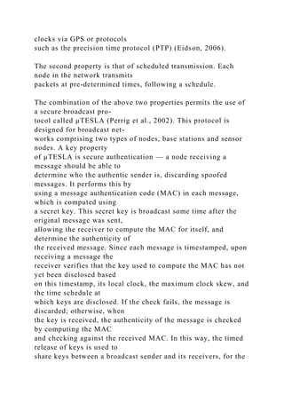
The field of cryptography is one of the cornerstones of security
and privacy. The word
“cryptography” is derived from the Latin roots “crypt” meaning
secret and “graphia”
meaning write, and thus literally means “the study of secret
writing.”
We begin with a review of the basic cryptographic primitives
for encryption and de-
cryption, secure hashing, and authentication. Issues that are
particularly relevant for the
design and analysis of embedded and cyber-physical systems are
highlighted. The reader
is warned that examples given in this chapter, particularly those
listing code, are given at
a high level of abstraction, and omit details that are critical to
developing secure crypto-
graphic implementations. See books such as (Menezes et al.,
1996; Ferguson et al., 2010)
for a more in-depth treatment of the subject.
17.1.1 Encryption and Decryption
Encryption is the process of translating a message into an
encoded form with the intent
that an adversary cannot recover the former from the latter. The
original message is
typically referred to as the plaintext, and its encoded form as
the ciphertext. Decryption
is the process of recovering the plaintext from the ciphertext.
The typical approach to encryption relies on the presence of a
secret called the key. An
encryption algorithm uses the key and the plaintext in a
prescribed manner to obtain the

ciphertext. The key is shared between the parties that intend to
exchange a message se-
curely. Depending on the mode of sharing, there are two broad
categories of cryptography.
17.1. CRYPTOGRAPHIC PRIMITIVES
In symmetric-key cryptography, the key is a single entity that is
known to both sender
and receiver. In public-key cryptography, also termed
asymmetric cryptography, the
key is split into two portions, a public part and a private part,
where the public key is
known to everyone (including the adversary) and the private key
is known only to the re-
ceiver. In the rest of this section, we present a brief
introduction to these two approaches
to cryptography.
One of the fundamental tenets of cryptography, known as
Kerckhoff’s principle, states
that a cryptographic system (algorithm) should be secure even if
everything about the sys-
tem, except the key, is public knowledge. In practical terms,
this means that even if the
adversary knows all details about the design and implementation
of a cryptographic algo-
rithm, as long as he does not know the key, he should be unable
to recover the plaintext
from the ciphertext.

Symmetric-Key Cryptography
Let Alice and Bob be two parties that seek to communicate with
each other securely. In
symmetric-key cryptography, they accomplish this using a
shared secret key K. Suppose
Alice wishes to encrypt and send Bob an n-bit plaintext
message,M = m1m2m3 . . .mn ∈
{0, 1}n. We wish to have an encryption scheme that, given the
shared key K, should en-
code M into ciphertext C with the following two properites.
First, the intended recipient
Bob should be able to easily recover M from C. Second, any
adversary who does not
know K should not, by observing C, be able to gain any more
information about M .
We present intuition for the operation of symmetric-key
cryptography using a simple,
idealized scheme known as the one-time pad. In this scheme, the
two parties Alice and
Bob share an n-bit secret key K = k1k2k3 . . . kn ∈ {0, 1}n,
where the n bits are chosen
independently at random. K is known as the one-time pad.
Given K, encryption works
by taking the bit-wise XOR of M and K; i.e., C = M ⊕K where⊕
denotes XOR. Alice
then sends C over to Bob, who decrypts C by taking the bit-wise
XOR of C with K;
using properties of the XOR operation, C ⊕K = M .
Suppose an adversary Eve observes C. We claim that Eve has no
more information about
M or K than she had without C. To see this, fix a plaintext
message M . Then, every
unique ciphertext C ∈ {0, 1}n can be obtained from M with a

corresponding unique
choice of keyK — simply setK = C⊕M where C is the desired
ciphertext. Put another
way, a uniformly random bit-stringK ∈ {0, 1}n generates a
uniformly random ciphertext
C ∈ {0, 1}n. Thus, looking at this ciphertext, Eve can do no
better than guessing at the
value of K uniformly at random.
Notice that Alice cannot use the key K more than once!
Consider what happens if she
does so twice. Then Eve has access to two ciphertexts C1 =
M1⊕K and C2 = M2⊕K.
If Eve computes C1 ⊕ C2, using properties of XOR, she learns
M1 ⊕M2. Thus, Eve
receives partial information about the messages. In particular, if
Eve happens to learn
one of the messages, she learns the other one, and can also
recover the key K. Thus, this
scheme is not secure if the same key is used for multiple
communications, hence the name
“one-time pad.” Fortunately, other, stronger symmetric key
cryptography schemes exist.
Most common symmetric key encryption methods use a building
block termed a block
cipher. A block cipher is an encryption algorithm based on
using a k-bit key K to

convert an n-bit plaintext message M into an n-bit ciphertext C.
It can be mathemati-
cally captured in terms of an encryption function E : {0, 1}k ×
{0, 1}n → {0, 1}n; i.e.,
E(K,M) = C. For a fixed key K, the function EK defined by
EK(M) = E(K,M)
must be a permutation from {0, 1}n to {0, 1}n. Decryption is
the inverse function of
encryption; note that the inverse exists for each K as EK is
invertible. We denote the
decryption function corresponding to EK by DK = E−1K . Note
that for simplicity this
model of encryption abstracts it to be (only) a function of the
message and the key; in
practice, care must be taken to use a suitable block cipher mode
that, for example, does
not always encrypt the same plaintext to the same ciphertext.
One of the classic block ciphers is the data encryption standard
(DES). Introduced in
the mid-1970s, DES was the first block cipher based on modern
cryptographic techniques,
considered to be “commercial-grade,” with an open
specification. While the details of
DES are beyond the scope of this chapter, we note that versions
of DES are still used
in certain embedded devices. For instance, a version of DES,
known as 3DES, which
involves applying the DES algorithm to a block three times, is
used in certain “chip and
PIN” payment cards around in the world. The basic version of
the DES involves use
of a 56-bit key and operates on 64-bit message blocks. While
DES initially provided
an acceptable level of security, by the mid-1990s, it was getting
easier to break it using

“brute-force” methods. Therefore, in 2001, the U.S. National
Institute of Standards and
Technology (NIST) established a new cryptographic standard
known as the advanced
encryption standard or AES. This standard is based on a
cryptographic scheme called
Rijndael proposed by Joan Daemen and Vincent Rijmen, two
researchers from Belgium.
AES uses a message block length of 128 bits and three different
key lengths of 128, 192,
and 256 bits. Since its adoption, AES has proved to be a strong
cryptographic algorithm
amenable to efficient implementation both in hardware and in
software. It is estimated
that the current fastest supercomputers could not successfully
mount a brute-force attack
on AES within the estimated lifetime of the solar system!
Public-Key Cryptography
In order to use symmetric-key cryptography, Alice and Bob
need to have already set up
a shared key in advance. This is not always easy to arrange.
Public-key cryptography is
designed to address this limitation.
In a public-key cryptosystem, each principal (Alice, Bob, etc.)
has two keys: a public key,

known to everyone, and a private key, known only to that
principal. When Alice wants
to send Bob a secret message, she obtains his public key KB and
encrypts her message
with it. When Bob receives the message, he decrypts it with his
private key kB . In
other words, the encryption function based onKB must be
invertible using the decryption
function based on kB , and moreover, must not be invertible
without kB .
Let us consider the last point. Encryption using a public key
must effectively be a one-
way function: a publicly-known function F such that it is easy
to compute F (M) but
(virtually) impossible to invert without knowledge of a suitable
secret (the private key).
Remarkably, there is more than one public-key cryptographic
scheme available today,
each based on a clever combination of mathematics, algorithm
design, and implementa-
tion tricks. We focus our attention here on one such scheme
proposed in 1978 (Rivest
et al.), known as RSA for the initials of its creators: Rivest,
Shamir and Adleman. For
brevity, we mostly limit our discussion to the basic
mathematical concepts behind RSA.
Consider the setting where Bob wishes to create his public-
private key pair so that others
can send him secret messages. The RSA scheme involves three
main steps, as detailed
below:
1. Key Generation: Select two large prime numbers p and q, and
compute their prod-

uct n = pq. Then compute ϕ(n) where ϕ denotes Euler’s totient
function. This
function maps an integer n to the number of positive integers
less than or equal
to n that are relatively prime to n. For the special case of the
product of primes,
ϕ(n) = (p−1)(q−1). Select a random integer e such that 1 < e <
ϕ(n) such that
the greatest common divisor of e and ϕ(n), denoted GCD(e,
ϕ(n)) equals 1. Then
compute d, 1 < d < ϕ(n), such that ed ≡ 1 (mod ϕ(n)). The key
generation
process is now complete. Bob’s public key KB is the pair (n, e).
The private key is
kB = d.
2. Encryption: When Alice wishes to send a message to Bob,
she first obtains his
public key KB = (n, e). Given the message M to transmit, she
computes the
ciphertext C as C = M e (mod n). C is then transmitted to Bob.
3. Decryption: Upon receipt of C, Bob computes Cd (mod n). By
properties of
Euler’s totient function and modular arithmetic, this quantity
equals M , allowing
Bob to recover the plaintext message from Alice.
We make two observations on the above scheme. First, the

operations in the various
steps of RSA make heavy use of non-linear arithmetic on large
numbers, especially mod-
ular multiplication of large integers and modular
exponentiation. These operations must
be implemented carefully, especially on embedded platforms, in
order to operate effi-
ciently. For instance, modular exponentiation is typically
implemented using a version of
the square-and-multiply technique outlined in Example 16.1 of
Chapter 16. Second, the
effectiveness of the approach depends critically on
infrastructure to store and maintain
public keys. Without such a public-key infrastructure, an
attacker Eve can masquerade
as Bob, advertising her own public key as Bob’s, and thus
fooling Alice into sending her
messages intended for Bob. While such a public-key
infrastructure has now been estab-
lished for servers on the Web using so-called “certificate
authorities,” it is more challeng-
ing to extend that approach for networked embedded systems
for a variety of reasons: the
large scale of devices that may act as servers, the ad-hoc nature
of networks, and the re-
source constraints on many embedded devices.1 For this reason,
public-key cryptography
is not as widely used in embedded devices as is symmetric-key
cryptography.
17.1.2 Digital Signatures and Secure Hash Functions
The cryptographic primitives for encryption and decryption help
in providing confiden-
tiality of data. However, by themselves, they are not designed to
provide integrity or au-

thenticity guarantees. Those properties require the use of
related, but distinct, primitives:
digital signatures, secure hash functions, and message
authentication codes (MACs). This
section provides a brief overview of these primitives.
1Let’s Encrypt, an ongoing effort to develop a free, automated,
and open certificate authority might miti-
gate some of these challenges; see https://letsencrypt.org/ for
more details.
https://letsencrypt.org/
Secure Hash Functions
A secure hash function (also known as cryptographic hash
function) is a deterministic
and keyless function H : {0, 1}n → {0, 1}k that maps n-bit
messages to k-bit hash
values. Typically, n can be arbitrarily large (i.e., the message
can be arbitrarily long) while
k is a relatively small fixed value. For example, SHA-256 is a
secure hash function that
Implementation Matters for Cryptography
Embedded platforms typically have limited resources such as
memory or energy, and
must obey physical constraints, for instance on real-time
behavior. Cryptography can

be computationally quite demanding. Such computations cannot
simply be offloaded
“to the cloud” as secret data must be secured at the end point
before being sent out
on the network. Thus, cryptographic primitives must be
implemented in a manner that
obeys the constraints imposed by embedded platforms.
Consider, for example, public-key cryptography. These
primitives involve modu-
lar exponentiation and multiplications that can have large
timing, memory, and energy
requirements. Consequently, researchers have developed
efficient algorithms as well
as software and hardware implementations. A good example is
Montgomery mul-
tiplication (Montgomery, 1985), a clever way of performing
modular multiplication
by replacing the division (implicit in computing the modulus)
with addition. Another
promising technology is elliptic curve cryptography which
allows for a level of se-
curity comparable with the RSA approach with keys of smaller
bit-width, reducing the
memory footprint of implementations; see, for example, Paar
and Pelzl (2009) for de-
tails. Due to the costs of public-key cryptography, it is often
used to exchange a shared
symmetric key that is then used for all subsequent
communication.
Another important aspect of implementing cryptographic
schemes is the design and
use of random number generation (RNG). A high-quality RNG
requires as input a
source of randomness with high entropy. Many recommended

high entropy sources
involve physical processes, such atmospheric noise or atomic
decay, but these may not
be easy to use in embedded systems, especially in hardware
implementations. Alter-
natively, one can use on-chip thermal noise and the timing of
input events from the
physical world and network events. Polling the physical world
for many such sources
of randomness may consume power, leading to implementation
trade-offs; see Perrig
et al. (2002) for an example.
maps messages to a 256-bit hash, and is being adopted for
authenticating some software
packages and for hashing passwords in some Linux
distributions. For a message M , we
term H(M) as the “hash of M.”
A secure hash function H has certain important properties that
distinguishes it from more
traditional hash functions used for non-security purposes:
• Efficient to compute: Given a message M , it should be
efficient to compute H(M).
• Pre-image resistance: Given a hash (value) h, it should be
computationally infeasible
to find a message M such that h = H(M).

• Second pre-image resistance: Given a messageM1, it should be
computationally infea-
sible to find another message M2 such that H(M1) = H(M2).
This property prevents
attackers from taking a known message M1 and modifying it to
match a desired hash
value (and hence find the corresponding message M2).
• Collision resistance: It should be computationally infeasible to
find two different mes-
sages M1 and M2 where H(M1) = H(M2). This property, a
stronger version of
second pre-image resistance, prevents an attacker from taking
any starting message
and modifying it to match a given hash value.
A common use of secure hash functions is to verify the integrity
of a message or a piece of
data. For example, before you install a software update on your
computer you might want
to verify that the update you downloaded is a valid copy of the
package you are updating
and not something modified by an attacker. Providing a secure
hash of the software update
on a separate channel than the one on which the update file is
distributed can provide such
assurance. After separately downloading this hash value, you
can verify, by computing
the hash yourself on the software, that the provided hash indeed
matches the one you
compute. With the growing trend for embedded systems to be
networked and to receive
software patches over the network, the use of secure hash
functions is expected to be a
central component of any solution that maintains system

integrity.
Digital Signatures
A digital signature is a cryptographic mechanism, based on
public-key cryptography, for
the author of a digital document (message) to authenticate
himself/herself to a third party
and to provide assurance about the integrity of the document.
The use of digital signatures
involves the following three stages:
1. Key generation: This step is identical to the key generation
phase of public-key
cryptosystems, resulting in a public key-private key pair.
2. Signing: In this step, the author/sender digitally signs the
document to be sent to
the receiving party.
3. Verification: The recipient of a signed document verifies,
using the digital signature,
that the sender of the document is indeed who he/she purports to
be.
We now illustrate how the basic scheme works for the RSA
cryptosystem. Suppose
Bob wishes to digitally sign a message M before sending it to
Alice. Recall from Sec-

tion 17.1.1 that, using RSA, Bob can generate his public key as
KB = (n, e) and private
key kB = d. One simple authentication scheme is for Bob to use
his key-pair in reverse:
to sign M , he simply encrypts it with his private key,
computing S = Md (mod n), and
sends S to Alice along with M . When Alice receives this signed
message, she uses KB
to recover M from the signature S and verifies it by comparing
it with the received mes-
sage. If they match, the message has been authenticated;
otherwise, Alice has detected
tampering either in the message or its signature.
The above scheme is simple, but flawed. In particular, given the
signatures S1 and S2 for
two messages M1 and M2, notice that an attacker can construct
the signature for message
M1 ·M2 by simply multiplying together S1 and S2 (mod n). In
order to guard against
this attack, one can first compute a secure hash of M1 and M2
before computing the
signatures on the resultant hashes rather than on the messages.
Message Authentication Codes
A message authentication code (MAC) is a cryptographic
mechanism, based on
symmetric-key cryptography, for providing integrity and
authenticity to a document. It is
thus the symmetric-key analog of a digital signature. As in other
symmetric-key schemes,
the use of a MAC requires first setting up a shared key between
sender and receiver that
each of them can use to authenticate messages sent by the other.
For this reason, MACs

are best suited to settings where such a shared key can be easily
set up. For instance,
modern automobiles comprise multiple electronic control units
(ECUs) communicating
with each other on an on-board network such as a controller-
area network (CAN) bus.
In this case, if each ECU is pre-programmed with a common
key, then each ECU can
authenticate messages sent from other ECUs on the CAN bus
using MACs.
17.2 Protocol and Network Security
An attacker typically gains access to a system via its connection
to a network or some
other medium used to connect it with other components.
Additionally, it is increasingly
the case that a single embedded system comprises many
distributed components con-
nected over a network. Thus, one must address fundamental
questions about security
over a network and using various communication protocols, a
field termed protocol se-
curity or network security. In this section, we review basic
ideas related to two topics
of particular relevance for embedded systems: key exchange and
cryptographic protocol
design.

17.2.1 Key Exchange
We have already seen how secret keys are critical components
of both symmetric and
asymmetric cryptosystems. How are these keys established in
the first place? In a sym-
metric cryptosystem, we need a mechanism for two
communicating parties to agree on a
single shared key. In an asymmetric cryptosystem, we need
infrastructure for establish-
ing and maintaining public keys so that any party on a network
can look up the public
key of any other party it wishes to communicate with. In this
section, we discuss a classic
method for key exchange and some alternative schemes
customized to specific embedded
system design problems, with a focus on symmetric
cryptography.
Diffie-Hellman Key Exchange
In 1976, Whitfield Diffie and Martin Hellman introduced what
is widely considered the
first public-key cryptosystem (Diffie and Hellman, 1976). The
crux of their proposal was
a clever scheme for two parties to agree on a shared secret key
using a communication
medium observable by anyone. This scheme is commonly
referred to as Diffie-Hellman
key exchange.
Suppose there are two parties Alice and Bob that wish to agree
on a secret key. Everything
Alice sends to Bob, and vice-versa, can be viewed by an
attacker Eve. Alice and Bob wish
to agree on a key while ensuring that it is computationally

infeasible for Eve to compute
that key by observing their communication. Here is how Alice
and Bob can use Diffie-
Hellman key exchange to achieve this objective.
17.2. PROTOCOL AND NETWORK SECURITY
To begin with, Alice and Bob need to agree on two parameters.
In doing so, they can use
various methods including a hard-coded scheme (e.g., a
parameter hard-coded into the
same program they use) or one of them can announce the
parameters to the other in some
deterministic fashion (e.g., based on a fixed ordering between
their network addresses).
The first parameter is a very large prime number p. The second
is a number z such that
1 < z < p− 1. Note that an attacker can observe z and p.
After these parameters p and z are agreed upon, Alice randomly
selects a number a from
the set {0, 1, . . . , p − 2} and keeps it secret. Similarly, Bob
randomly selects a number
b ∈ {0, 1, . . . , p − 2} and keeps it secret. Alice computes the
quantity A = za (mod p)
and sends it to Bob. Likewise, Bob computes B = zb (mod p)
and sends it to Alice. In
addition to z and p, the attacker Eve can observe A and B, but
not a and b.
On receiving B, Alice uses her secret number a to compute Ba

(mod p). Bob performs
the analogous step, computing Ab (mod p). Now, observe that
Ab (mod p) = zab (mod p) = Ba (mod p)
Thus, amazingly, Alice and Bob have agreed on a shared key K
= zab (mod p) simply
by communicating on a public channel. Note that they have
revealed neither of the secret
numbers a or b to the attacker Eve. Without knowledge of a or
b, Eve cannot reliably
compute K. Moreover, it is computationally very difficult for
Eve to compute a or b sim-
ply by knowing p, z, A or B, since the underlying problem is
one known as the discrete
logarithm problem, for which no efficient (polynomial-time)
algorithm is known. Put
another way, the function f(x) = zx (mod p) is a one-way
function.
Diffie-Hellman is simple, elegant, and effective: unfortunately,
it is typically not practical
for resource-constrained embedded systems. Computing it
involves modular exponen-
tiation for large primes (typical key sizes range to 2048-bits),
and thus impractical for
energy-constrained platforms that must obey real-time
constraints. We therefore discuss
next a few alternative schemes.
Timed Release of Keys
Many networked embedded systems use a broadcast medium for
communication — one
where senders send data over a public channel where all
receivers, intended and unin-

tended, can read that data. Examples include on-board
automotive networks using the
CAN bus and wireless sensor networks. A broadcast medium
has many advantages: it
is simple, requires little infrastructure, and a sender can quickly
reach a large number of
receivers. However, it also has certain disadvantages, notably
that malicious parties can
eavesdrop and inject malicious packets with ease. Reliability of
the broadcast medium
can also be concern.
How can one achieve secure key exchange in such a broadcast
medium, under constraints
on timing and energy consumption? This question was studied
in the early 2000s, when
the first work was done on deploying wireless sensor networks
(e.g., see Perrig et al.
(2004); Perrig and Tygar (2012)). One of the novel ideas is to
leverage timing properties
of these networks, an idea whose roots go back to a paper by
Anderson et al. (1998).
The first property is that of clock synchronization, where
different nodes on the network
have clocks such that the difference between the values of any
two clocks is bounded by
a small constant. Many sensor nodes can have synchronized

clocks via GPS or protocols
such as the precision time protocol (PTP) (Eidson, 2006).
The second property is that of scheduled transmission. Each
node in the network transmits
packets at pre-determined times, following a schedule.
The combination of the above two properties permits the use of
a secure broadcast pro-
tocol called µTESLA (Perrig et al., 2002). This protocol is
designed for broadcast net-
works comprising two types of nodes, base stations and sensor
nodes. A key property
of µTESLA is secure authentication — a node receiving a
message should be able to
determine who the authentic sender is, discarding spoofed
messages. It performs this by
using a message authentication code (MAC) in each message,
which is computed using
a secret key. This secret key is broadcast some time after the
original message was sent,
allowing the receiver to compute the MAC for itself, and
determine the authenticity of
the received message. Since each message is timestamped, upon
receiving a message the
receiver verifies that the key used to compute the MAC has not
yet been disclosed based
on this timestamp, its local clock, the maximum clock skew, and
the time schedule at
which keys are disclosed. If the check fails, the message is
discarded; otherwise, when
the key is received, the authenticity of the message is checked
by computing the MAC
and checking against the received MAC. In this way, the timed
release of keys is used to
share keys between a broadcast sender and its receivers, for the

purpose of authenticating
messages.
A similar approach has been adopted for CAN-based automotive
networks. Lin et al.
(2013) have shown how to extend the µTESLA approach for the
CAN bus where the
nodes do not necessarily share a common global notion of time.
Timed delayed release
17.2. PROTOCOL AND NETWORK SECURITY
of keys has also been implemented for Time Triggered Ethernet
(TTE) (Wasicek et al.,
2011).
Other Schemes
In certain application domains, customized schemes have been
developed for key ex-
change using special characteristics of those domains. For
instance, Halperin et al. (2008)
discuss a key exchange scheme for implantable medical devices
(IMDs) such as pace-
makers and defibrillators. They propose a “zero-power” security
mechanism on the im-
planted device based on radio-frequency (RF) power harvesting.
The novel key exchange
scheme involves a “programmer” device initiating
communication with the IMD (and
supplying an RF signal to power it). The IMD generates a

random value that is commu-
nicated as a weak modulated sound wave that is perceptible by
the patient. The security
Reverse Engineering Systems to Improve Security
Several embedded systems were designed at a time when
security was a secondary
design concern, if one at all. In recent years, researchers have
shown how this lack of
attention to security can lead to compromised systems in
various domains. The chief
approach taken is to reverse engineer protocols that provide
access to systems and the
working of their components.
We present here three representative examples of vulnerabilities
demonstrated in
real embedded systems. Halperin et al. (2008) show how
implantable medical devices
(IMDs) can be read and reprogrammed wirelessly. Koscher et
al. (2010) demonstrate
for automobiles how the on-board diagnostics bus (OBD-II)
protocol can be subverted
to adversarially control a wide range of functions, including
disabling the brakes and
stopping the engine. Ghena et al. (2014) study traffic light
intersections and show
how their functioning can be partially controlled wirelessly to
perform, for example, a
denial-of-service attack causing traffic congestion.
Such investigations based on reverse engineering “legacy”
embedded systems to un-
derstand their functioning and uncover potential security flaws
form an important part

of the process of securing our cyber-physical infrastructure.
of this scheme relies on a threat model based on physical
security around the patient’s
immediate vicinity, one that is plausible for this particular
application.
17.2.2 Cryptographic Protocol Design
Some of the most-publicized vulnerabilities in networked
embedded systems, at the time
of writing, arise from the fact that the communication protocols
were designed with little
or no security in mind (see the box on page 472). However,
even protocols designed for
security using cryptographic primitives can have vulnerabilities.
Poor protocol design can
compromise confidentiality, integrity, and authenticity
properties even if one assumes per-
fect cryptography and the presence of key exchange and key
management infrastructure.
We explain this point with an example.
Example 17.1: A replay attack on a protocol is one where an
attacker is able to
violate a security property by replaying certain messages in the
protocol, possibly
with modifications to accompanying data.

We describe here a replay attack on a fictitious wireless sensor
network protocol.
This network comprises a base station S and several energy-
constrained sensor
nodes N1, N2, . . . , Nk communicating via broadcast. Each
node spends most of
its time in a sleep mode, to conserve energy. When S wants to
communicate with
a particular node Ni to take a sensor reading, it sends it a
message M encrypted
with a suitable shared key Ki pre-arranged between S and Ni. Ni
then responds
with an encrypted sensor reading R. In other words, the protocol
has a message
exchange as follows:
S → Ni : E(Ki,M)
Ni → S : E(Ki, R)
This protocol, on the face of it, seems secure. However, it has a
flaw that can
hinder operation of the network. Since the nodes use broadcast
communication,
an attacker can easily record the messageE(Ki,M). The attacker
can then replay
this message multiple times at a low power so that it is detected
by Ni, but not by
S. Ni will keep responding with encrypted sensor readings,
possibly causing it
to run down its battery much faster than anticipated, and
disabling its operation.
Notice that there was nothing wrong with the individual
cryptographic steps used
in this protocol. The problem was with the temporal behavior of
the system —

17.3. SOFTWARE SECURITY
that Ni had no way of checking if a message is “fresh.” A
simple countermeasure
to this attack is to attach a fresh random value, called a nonce,
or a timestamp
with each message.
This attack is also an example of a so-called denial-of-service
attack, abbre-
viated DoS attack, indicating that the impact of the attack is a
loss of service
provided by the sensor node.
Fortunately, techniques and tools exist to formally model
cryptographic protocols and ver-
ify their correctness with respect to specific properties and
threat models before deploying
them. More widespread use of these techniques is needed to
improve protocol security.
17.3 Software Security
The field of software security is concerned with how errors in
the software implementa-
tion can impact desired security and privacy properties of the
system. Bugs in software
can and have been used to steal data, crash a system, and worse,
allow an attacker to obtain
an arbitrary level of control over a system. Vulnerabilities in

software implementations
are one of the largest categories of security problems in
practice. These vulnerabilities
can be especially dangerous for embedded systems. Much of
embedded software is pro-
grammed in low-level languages such as C, where the
programmer can write arbitrary
code with few language-level checks. Moreover, the software
often runs “bare metal”
without an underlying operating system or other software layer
that can monitor and trap
illegal accesses or operations. Finally, we note that in embedded
systems, even “crashing”
the system can have severe consequences, since it can
completely impair the interaction
of the system with the physical world. Consider, for example, a
medical device such as a
pacemaker, where the consequences of a crash may be that the
device stops functioning
(e.g. pacing), leading to potentially life-threatening
consequences for the patient.
In this section, we give the reader a very brief introduction to
software security problems
using a few illustrative examples. The reader is referred to
relevant books on security
(e.g., Smith and Marchesini (2007)) for further details.
Our examples illustrate a vulnerability known as a buffer
overflow or buffer overrun.
This class of errors is particularly common in low-level
languages such as C. It arises from

the absence of automatic bounds-checking for accessing arrays
or pointers in C programs.
More precisely, a buffer overflow is a error arising from the
absence of a bounds check
resulting in the program writing past the end of an array or
memory region. Attackers can
use this out-of-bounds write to corrupt trusted locations in a
program such as the value
of a secret variable or the return address of a function. (Tip:
material in Chapter 9 on
Memory Architectures might be worth reviewing.) Let us begin
with a simple example.
Example 17.2: The sensors in certain embedded systems use
communication
protocols where data from various on-board sensors is read as a
stream of bytes
from a designated port or network socket. The code example
below illustrates one
such scenario. Here, the programmer expects to read at most 16
bytes of sensor
data, storing them into the array sensor data.
1 char sensor_data[16];
2 int secret_key;
3
4 void read_sensor_data() {
5 int i = 0;
6
7 // more_data returns 1 if there is more data,

8 // and 0 otherwise
9 while(more_data()) {
10 sensor_data[i] = get_next_byte();
11 i++;
12 }
13
14 return;
15 }
The problem with this code is that it implicitly trusts the sensor
stream to be no
more than 16 bytes long. Suppose an attacker has control of that
stream, either
through physical access to the sensors or over the network.
Then an attacker can
provide more than 16 bytes and cause the program to write past
the end of the
array sensor data. Notice further how the variable secret key is
defined
right after sensor data, and assume that the compiler allocates
them adja-
cently. In this case, an attacker can exploit the buffer oveflow
vulnerability to
provide a stream of length 20 bytes and overwrite secret key
with a key of
his choosing. This exploit can then be used to compromise the
system in other
ways.

17.3. SOFTWARE SECURITY
The example above involves an out-of-bounds write in an array
stored in global memory.
Consider next the case when the array is stored on the stack. In
this case, a buffer overrun
vulnerability can be exploited to overwrite the return address of
the function, and cause it
to execute some code of the attacker’s choosing. This can lead
to the attacker gaining an
arbitrary level of control over the embedded system.
Example 17.3: Consider below a variant on the code in Example
17.2 where
the sensor data array is stored on the stack. As before, the
function reads
a stream of bytes and stores them into sensor data. However, in
this case,
the read sensor data is then processed within this function and
used to set certain
globally-stored flags (which can then be used to take control
decisions).
1 int sensor_flags[4];
2
3 void process_sensor_data() {
4 int i = 0;
5 char sensor_data[16];
6
7 // more_data returns 1 if there is more data,
8 // and 0 otherwise
9 while(more_data()) {
10 sensor_data[i] = get_next_byte();

11 i++;
12 }
13
14 // some code here that sets sensor_flags
15 // based on the values in sensor_data
16
17 return;
18 }
Recall from Chapter 9 how the stack frame of a function is laid
out. It is possi-
ble for the return address of function process sensor data to be
stored in
memory right after the end of the array sensor data. Thus, an
attacker can
exploit the buffer overflow vulnerability to overwrite the return
address and cause
execution to jump to a location of his choice. This version of
the buffer overflow
exploit is sometimes (and rather aptly) termed as stack
smashing.
Moreover, the attacker could write a longer sequence of bytes to
memory and
include arbitrary code in that sequence. The overwritten return
address could be

tailored to be within this overwritten memory region, thus
causing the attacker
to control the code that gets executed! This attack is often
referred to as a code
injection attack.
How do we avoid buffer overflow attacks? One easy way is to
explicitly check that we
never write past the end of the buffer, by keeping track of its
length. Another approach
is to use higher-level languages that enforce memory safety —
preventing the program
from reading or writing to locations in memory that it does not
have privileges for or that
the programmer did not intend it to. Exercise 1 gives you some
practice with writing code
so as to avoid a buffer overflow.
17.4 Information Flow
Many security properties specify restrictions on the flow of
information between princi-
pals. Confidentiality properties restrict the flow of secret data
to channels that are readable
by an attacker. For example, your bank balance should be
viewable only by you and au-
thorized bank personnel and not by an attacker. Similarly,
integrity properties restrict the
flow of untrusted values, controlled by an attacker, to trusted
channels or locations. Your
bank balance should be writable only by trusted deposit or
withdrawal operations and not
arbitrarily by a malicious party. Thus, secure information flow,
the systematic study of
how the flow of information in a system affects its security and
privacy, is a central topic

in the literature.
Given a component of an embedded system it is important to
understand how informa-
tion flows from secret locations to attacker-readable “public”
locations, or from attacker-
controlled untrusted channels to trusted locations. We need
techniques to detect illegal
information flows and to quantify their impact on the overall
security of the system. Addi-
tionally, given security and privacy policies, we need
techniques to enforce those policies
on a system by suitably restricting the flow of information. Our
goal, in this section, is to
equip the reader with the basic principles of secure information
flow so as to be able to
develop such techniques.
17.4. INFORMATION FLOW
17.4.1 Examples
In order to motivate the secure information flow problem, we
present a series of examples.
Although these examples focus on confidentiality, the same
approaches and concerns ap-
ply for integrity properties as well.
Example 17.4: Medical devices are increasingly software-
controlled, personal-
ized, and networked. An example of such a device is a blood

glucose meter, used
by doctors and patients to monitor a patient’s blood glucose
level. Consider a hy-
pothetical glucose meter that can take a reading of a patient’s
glucose level, show
it on the device’s display, and also transmit it over the network
to the patient’s
hospital. Here is a highly-abstracted version of the software that
might perform
these tasks.
1 int patient_id; // initialized to the
2 // patient’s unique identifier
3 void take_reading() {
4 float reading = read_from_sensor();
5
6 display(reading);
7
8 send(network_socket, hospital_server,
9 reading, patient_id);
10
11 return;
12 }
The function take reading records a single blood glucose
reading (e.g., in
mg/dL) and stores it in a floating-point variable reading. It then
writes this
value, suitably formatted, to the device’s display. Finally, it
transmits the value
along with the patient’s ID without any encryption over the
network to the hospital

server for analysis by the patient’s doctor.
Suppose that the patient wishes to have his glucose level kept
private, in the sense
that its value is known only to him and his doctor, but no one
else. Does this
program achieve that objective? It is easy to see that it does not,
as the value
of reading is transmitted “in the clear” over the network. We
can formal-
ize this violation of privacy as an illegal information flow from
reading to
network socket, where the former is a secret location whereas
the latter is a
public channel visible to an attacker.
With the knowledge of cryptographic primitives presented
earlier in this chapter, we know
that we can do better. In particular, let us assume the presence
of a shared key between the
patient’s device and the hospital server that permits the use of
symmetric-key encryption.
Consider the following new version of the above example.
Example 17.5: In this version of the program, we employ
symmetric-key cryp-
tography, denoted by AES, to protect the reading. The
encryption process is ab-
stractly represented by the function enc AES, and send enc

differs from send
only in the type of its third argument.
3 long cipher_text;
4
5 struct secret_key_s {
6 long key_part1; long key_part2;
7 }; // struct type storing 128-bit AES key
8
9 struct secret_key_s secret_key; // shared key
10
11 void take_reading() {
12 float reading = read_from_sensor();
13
14 display(reading);
15
16 enc_AES(&secret_key, reading, &cipher_text);
17
18 send_enc(network_socket, hospital_server,
19 cipher_text, patient_id);
20
21 return;
22 }
In this case, there is still a flow of information from reading to
network socket. In fact, there is also a flow from secret key to
network socket. However, both these flows passed through an

encryption
function denoted by enc AES. In the security literature, such a
function is termed
a declassifier since it encodes the secret data in such a way that
it becomes accept-
able to transmit the encoded, “declassified” result to an
attacker-readable channel.
In other words, the declassifier serves as a “dam” blocking the
flow of secret infor-
mation and releasing only information that, by the properties of
the cryptographic
primitives, provides attackers with no more information than
they had before the
release.
While the above fix to the code blocks the flow of information
about the reading of the
patient’s blood glucose, note that it does not completely protect
the program. In particular,
notice that the patient’s ID is still being sent in the clear over
the network! Thus, even
though the attacker cannot tell, without the secret key, what the
patient’s reading is, he/she
knows who transmitted a reading to the hospital (and possibly
also at what time). Some
private data is still being leaked. One solution to this leak is
fairly obvious – we can
encrypt both variables reading and patient id using the secret

key before sending
them over the network.
So far we have assumed an implicit threat model where the
attacker can only read in-
formation sent over the network. However, for many embedded
systems, attackers may
also have physical access to the device. For instance, consider
what happens if the patient
loses his device and an unauthorized person (attacker) gains
access to it. If the patient’s
readings are stored on the device, the attacker might be able to
read the data stored on it
if such an illegal information flow exists. One approach to
guard against this attack is to
have the patient create a password, much like one creates a
password for other personal
devices, and have the device prompt one for the password when
turned on. This idea is
discussed in the example below.
Example 17.6: Suppose that a log of the past 100 readings is
stored
on the device. The code below sketches an implementation of a
function
show readings that prompts the user for an integer password,
and displays
the stored readings only if the current password stored in
patient pwd is en-
tered, otherwise displaying an error message that has no
information about the
stored readings.
3 int patient_pwd; // stored patient password

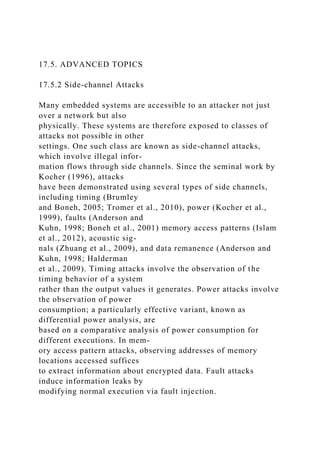
4
5 float stored_readings[100];
6
7 void show_readings() {
8 int input_pwd = read_input(); // prompt user for
9 // password and read it
10 if (input_pwd == patient_pwd) // check password
11 display(&stored_readings);
12 else
13 display_error_mesg();
14
15 return;
16 }
Assuming the attacker does not know the value of patient pwd,
we can see
that the above code does not leak any of the 100 stored
readings. However, it
does leak one bit of information: whether the input password
provided by the
attacker equals the correct password or not. In practice, such a
leak is deemed
acceptable since, for a strong choice of patient password, it
would take even the

most determined attacker an exponential number of attempts to
log in success-
fully, and this can be thwarted by disallowing more than a
small, fixed number of
attempts to provide the correct password.
The above example illustrates the concept of quantitative
information flow (QIF). QIF
is typically defined using a function measuring the amount of
information flowing from
a secret location to a public location. For instance, one might be
interested in computing
the number of bits leaked, as illustrated by the example above.
If this quantity is deemed
small enough, the information leak is tolerated, otherwise, the
program must be rewritten.
However, the code in Example 17.6 has a potential flaw. Once
again, this flaw stems
from a corresponding threat model. In particular, consider the
case where an attacker not
only has physical possession of the device, but also has the
knowledge and resources to
perform invasive attacks by opening up the device, and reading
out the contents of main
memory as it executes. In this case, the attacker can read the
value of patient pwd
simply by booting up the device and reading out the contents of
memory as the system is
initialized.
How can we protect against such invasive attacks? One
approach involves the use of se-
cure hardware or firmware coupled with secure hash functions.
Suppose the hardware
provides for secure storage where a secure hash of the user

password can be written out,
and any tampering detected. Then, only the secure hash need be
stored in main memory,
not the actual password. By the properties of a secure hash
function, it would be compu-
tationally infeasible for an attacker to reverse engineer the
password simply by knowing
the hash.
A similar flaw exists in Example 17.5, where the secret key is
stored in memory in the
clear. However, in this case, simply taking a secure hash of the
key is insufficient as the
actual key is required to perform encryption and decryption to
facilitate secure commu-
nication with the server. How do we secure this function? In
general, this requires an
additional component such as a secure key manager, e.g.,
implemented in hardware or by
a trusted operating system, one that uses a master key to encrypt
or decrypt the secret key
for the application.
Finally, although our examples illustrate the flow of
information through values of vari-
ables in software, information can also be leaked through other
channels. The term side
channel is used to refer to a channel that involves a non-

traditional way of communicat-
ing information, typically using a physical quantity such as
time, power consumption, or
the amplitude and frequency of an audio signal, or a physical
modification to the system,
such as a fault, that induces a traditional information leak. We
cover some basic concepts
on side-channel attacks in Section 17.5.2.
17.4.2 Theory
So far we have spoken of confidentiality and integrity
properties only informally. How
can we state these properties precisely, similar to the notation
introduced in Chapter 13?
It turns out that specifying security and privacy properties
formally can be quite tricky.
Various formalisms have been proposed in the literature over
the years, and there is no
consensus on a common definition of notions such as
confidentiality or integrity. How-
ever, some foundational concepts and principles have emerged.
We introduce these basic
concepts in this section.
The first key concept is that of non-interference. The term non-
interference is used
to refer to any of a family of (security) properties that specify
how actions taken by one
or more principals can or cannot affect (“interfere with”)
actions taken by others. For
instance, for integrity properties, we require that actions of an
attacker cannot affect the
values of certain trusted data or computations. Similarly, for
confidentiality properties, we
require that the actions taken by an attacker cannot depend on

secret values (thus implying
that the attacker has no information about those secrets).
There are several variants of non-interference that are useful for
expressing different kinds
of security or privacy properties. In defining these, it is
customary to use the terms high
and low to denote two security levels. For confidentiality, the
high level denotes secret
data/channels and the low level denotes public data/channels.
For integrity, the high level
denotes trusted data/channels while the low level denotes
untrusted data/channels. Non-
interference is typically defined over traces of a system, where
each input, output, and
state element is classified as being either low or high.
The first variant we introduce is observational determinism
(McLean, 1992; Roscoe,
1995) which is defined as follows: if two traces of a system are
initialized to be in states
in which the low elements are identical, and they receive the
same low inputs, then that
implies that the low elements of all states and outputs in that
trace must be identical. Put
another way, the low parts of a system’s trace are deterministic
functions of the low initial
state and the low inputs, and nothing else. This, in turn, implies
that an attacker who

only controls or observes the low parts of a system’s trace
cannot infer anything about the
high parts.
Another variant is generalized non-interference (McLean, 1996)
which requires a sys-
tem to exhibit a set of traces with a special property: for any
two traces τ1 and τ2, there
must exist a newly-constructed trace τ3 such that, at each time
step in τ3, the high inputs
are the same as in τ1 and the low inputs, states, and outputs are
the same as in τ2. Intu-
itively, by observing the low states and outputs, an attacker
cannot tell if she is seeing the
high inputs as in τ1 or as they occur in τ2.
The different variants of non-interference, however, share
something in common. Math-
ematically, they are all hyperproperties (Clarkson and
Schneider, 2010). Formally, a
hyperproperty is a set of sets of traces. Contrast this definition
with the definition of
a property as a set of traces, as introduced in Chapter 13. The
latter is more accurately
called a trace property, as its truth value can be evaluated on a
single, standalone trace of
a system. The truth value of a hyperproperty, in contrast,
typically2 cannot be determined
by observing a single trace. One needs to observe multiple
traces, and compute a relation
between them, in order to determine if they together satisfy or
violate a hyperproperty.
Example 17.7: Consider the two state machines in Figure 17.1.
In both cases,
the state machine has one secret input s and one public output z.

Additionally,
2Clearly, every (trace) property has an equivalent
hyperproperty, which is why we use the adverb “typi-
cally.”
x=0 / 1
inputs: s, x : {0,1}
output: z : {0,1}
x=1 / 0
(a) M1
s = 0 / 1
input: s : {0,1}
output: z : {0,1}
s = 0 / 1
s = 1 / 0
s = 1 / 0
(b) M2
Figure 17.1: An example of a state machine satisfying

observational determinism
(a) and one that does not (b). Input s is a secret (high) input,
and output z is a
public (low) output.
M1 has a public input x. An attacker can directly read the value
of x and z but
not s.
State machine M1 satisfies observational determinism (OD). For
any input se-
quence, M1 produces a binary output sequence that depends
solely on the values
of the public input x and not on s.
However, M2 does not satisfy OD. For example, consider the
input sequence
1010ω. Then, the corresponding output sequence of M2 will be
0101ω. If the in-
put sequence is switched to 0101ω, then the output will
correspondingly change to
1010ω. The adversary can gain information about the input s
simply by observing
the output z.
17.4.3 Analysis and Enforcement
Several techniques have been developed to analyze and track
the flow of information in
software systems, and, in some cases, to enforce information
flow policies either at design
time or run time. We mention some of these methods below,
with the caveat that this is a
rapidly evolving area and our selection is meant to be
representative, not exhaustive.

Taint analysis. In taint analysis, the flow of information is
tracked using labels (“taint”)
attached to data items and by monitoring memory operations.
When an illegal informa-
tion flow is detected, a warning is generated. Taint analysis has
been mainly developed for
software systems. It can be performed statically, when software
is compiled, or dynam-
ically, at run time. For instance, for the code in Example 17.4,
taint analysis can detect
the flow of secret data from reading to network socket. At run
time, this can be
detected before the write to the network socket, and used to
raise a run-time exception or
other preventive action. Static taint analysis is a simple
concept, and easy to apply, but
can generate false alarms. Dynamic taint analysis is just as easy
and more precise, but im-
poses a run-time overhead. System designers must evaluate for
themselves the suitability
of either mechanism for their contexts.
Formal verification of information flow. Techniques for formal
verification, such as the
model checking methods covered in Chapter 15, can also be
adapted to verify secure infor-
mation flow. These methods usually operate after the original
analysis problem has been
reduced to one of checking a safety property on a suitably

constructed model (Terauchi
and Aiken, 2005). Compared to taint analysis, such methods are
much more precise, but
they also come at a higher computational cost. As these methods
are still rapidly evolving,
detailed coverage of these methods is beyond the scope of this
chapter at the present time.
Run-time enforcement of policies. The notion of taint allows
one to specify simple
information flow policies, such as disallowing the flow of secret
data to any public location
at all times. However, some security and privacy policies are
more complex. Consider,
for example, a policy that a person’s location is public some of
the time (e.g., while they
are at work or in a public space such as an airport), but is kept
secret at selected other
times (e.g., when they visit their doctor). Such a policy involves
a time-varying secret tag
on the variable storing the person’s location. The problem of
specifying, checking, and
enforcing such expressive policies is an active area of research.
17.5 Advanced Topics
Certain problems in security and privacy gain special
significance in the context of cyber-
physical systems. In this section, we review two of these
problems and highlight some of
the key issues.

17.5. ADVANCED TOPICS
17.5.1 Sensor and Actuator Security
Sensors and actuators form the interface between the cyber and
physical worlds. In many
cyber-physical systems, these components are easily observed
or controlled by an at-
tacker. Detecting attacks on these components and securing
them is therefore an impor-
tant problem. Central to both efforts is to develop realistic
threat models and mechanisms
to address those threats. We review two representative recent
efforts in the area of sensor
security.
Recent work has focused on attacks on analog sensors, i.e.,
developing threat models
for these attacks as well as countermeasures. The main mode of
attack is to employ
electromagnetic interference (EMI) to modify the sensed signal.
Two recent projects
have studied EMI attacks in different applications. Foo Kune et
al. (2013) investigate
EMI attacks at varying power and distances on implantable
medical devices and consumer
electronics. Shoukry et al. (2013) study the possibility of EMI
attacks that spoof sensor
values for certain types of automotive sensors. We present here
some basic principles
from both projects.
Threat Models
In the context of sensor security, EMI can be classified along

multiple dimensions. First,
such interference can be invasive, involving modification to the
sensor components, or
non-invasive, involving observation or remote injection of
spurious values. Second, it
can be unintentional (e.g., arising from lightning strikes or
transformers) or intentional
(injected by an attacker). Third, it can be high-power,
potentially injecting faults into or
disabling the sensor, or low-power, which simply injects false
values or modifies sensor
readings. These dimensions can be used to define informal
threat models.
Foo Kune et al. (2013) describe a threat model for intentional,
low-power, non-invasive
attacks. This combination of characteristics is amongst the
hardest to defend against,
since the low-power and non-intrusive nature of the attacks
makes it potentially hard to
detect. The researchers design two kinds of EMI attacks.
Baseband attacks inject signals
within the same frequency band in which the generated sensor
readings lie. They can be
effective on sensors that filter signals outside the operating
frequency band. Amplitude-
modulated attacks start with a carrier signal in the same
frequency band of the sensor and
modulate it with an attack signal. They can match the resonant
frequency of a sensor,
thus amplifying the impact of even a low-power attack signal.
They demonstrate how

these attacks can be performed on implantable cardiac devices,
injecting forged signals
in leads, inhibiting pacing, causing defibrillation, etc. from 1 to
2 meters away from the
device.
The threat model considered by Shoukry et al. (2013) is for
intentional, non-invasive
attacks, with a focus on anti-lock braking systems (ABS) in
automobiles. The magnetic
wheel speed sensors are attacked by placing a malicious
actuator in close proximity of
the sensor (mountable from outside the vehicle) that modifies
the magnetic field measured
by the ABS sensor. One form of the attack, in which the
actuator disrupts the magnetic
field but is not precisely controllable by the attacker, can be
“merely” disruptive. Its
impact is similar to unintentional, high-power EMI. The trickier
form of the attack is
a spoofing attack, where the ABS system is deceived into
measuring an incorrect but
precise wheel speed for one or more of the wheels. This is
achieved by implementing
an active magnetic shield around the actuator. The reader is
referred to the paper for
additional details. The authors show how their attack can be
mounted on real automotive
sensors, and demonstrate, in simulation, how the ABS system
can be tricked into making
an incorrect braking decision in icy road conditions, causing the
vehicle to slip off-road.

Countermeasures
Both of the projects mentioned above also discuss potential
countermeasures to the at-
tacks.
Foo Kune et al. (2013) consider a range of defenses, both
hardware-based and software-
based. Hardware or circuit-level approaches include shielding
the sensor, filtering the
input signals, and common mode noise rejection. However,
these methods are reported to
have limited effectiveness. Thus, software-based defenses are
also introduced, including
estimating the EMI level in the environment, adaptive filtering,
cardiac probing to see if
the sensed signals follow an expected pattern, reverting to safe
defaults, and notifying
the victim (patient) or physician about the possibility of an
attack to allow them to take
suitable actions to move away from the EMI source.
Shoukry et al 2015; 2016 take a somewhat different approach
that is rooted in control
theory and formal methods. The idea is to create a mathematical
model of the system and
of sensor attacks, and devise algorithms to identify subsets of
sensors that are attacked,
isolate them, and use the remaining (unattacked) sensors to
perform state estimation and
control.

17.5. ADVANCED TOPICS
17.5.2 Side-channel Attacks
Many embedded systems are accessible to an attacker not just
over a network but also
physically. These systems are therefore exposed to classes of
attacks not possible in other
settings. One such class are known as side-channel attacks,
which involve illegal infor-
mation flows through side channels. Since the seminal work by
Kocher (1996), attacks
have been demonstrated using several types of side channels,
including timing (Brumley
and Boneh, 2005; Tromer et al., 2010), power (Kocher et al.,
1999), faults (Anderson and
Kuhn, 1998; Boneh et al., 2001) memory access patterns (Islam
et al., 2012), acoustic sig-
nals (Zhuang et al., 2009), and data remanence (Anderson and
Kuhn, 1998; Halderman
et al., 2009). Timing attacks involve the observation of the
timing behavior of a system
rather than the output values it generates. Power attacks involve
the observation of power
consumption; a particularly effective variant, known as
differential power analysis, are
based on a comparative analysis of power consumption for
different executions. In mem-
ory access pattern attacks, observing addresses of memory
locations accessed suffices
to extract information about encrypted data. Fault attacks
induce information leaks by
modifying normal execution via fault injection.

While an exhaustive survey of side-channel attacks is outside
the scope of this book,
we illustrate, using the example below, how information can
leak through a timing side
channel.
Example 17.8: Consider the C implementation of modular
exponentiation given
as the modexp function of Example 16.1. In Figure 17.2 we
show how the exe-
cution time of modexp varies as a function of the value of
exponent. Recall
how the exponent usually corresponds to the secret key in
implementations of
public-key cryptosystems such as RSA or Diffie-Hellman.
Execution time is de-
picted in CPU cycles on the y axis, while the value of exponent
ranges from
0 to 15. The measurements are made on a processor
implementing the ARMv4
instruction set.
Notice that there are five clusters of measurements around 600,
700, 750, 850,
and 925 cycles respectively. It turns out that each cluster
corresponds to values of
exponent that, when represented in binary, have the same
number of bits set to
1. For example, the execution times for values 1, 2, 4 and 8,
each corresponding
to a single bit set to 1, are clustered around 700 CPU cycles.

550
600
650
700
750
800
850
900
950
0 1 2 3 4 5 6 7 8 9 10 11 12 13 14 15
R
un
tim
e
(c
yc
le
s)
Exponent

Modular Exponentiation Timing Graph
Figure 17.2: Timing data for the modexp function of Example
16.1. The graph
shows how execution time (in CPU cycles on the y-axis) for
modexp varies as a
function of the value of the 4-bit exponent (listed on the x-
axis).
17.6. SUMMARY
Thus, from simply observing the execution time of modexp and
nothing else,
and with some knowledge of the underlying hardware platform
(or access to it),
an attacker can infer the number of bits set to 1 in exponent,
i.e., in the secret
key. Such information can significantly narrow down the search
space for brute-
force enumeration of keys.
In Example 17.8, it is assumed that an attacker can measure the
execution time of a fairly
small piece of code such as modexp, embedded within a larger
program. Is this realistic?
Probably not, but it does not mean timing attacks cannot be
mounted. More sophisticated
methods are available for an attacker to measure execution time
of a procedure. For
instance, Tromer et al. (2010) show how AES can be broken

using a timing attack where
an attacker simply induces cache hits or misses in another
process (by writing to carefully
chosen memory locations within its own memory segment),
along with an indirect way of
measuring whether the victim process suffered a cache hit or a
cache miss. This can allow
the attacker to know if certain table entries were looked up
during the AES computation,
thereby allowing him to reconstruct the key.
Side-channel attacks remind us that security compromises are
often achieved by breaking
assumptions made by system designers. In designing an
embedded system, careful con-
sideration must be given to the assumptions one makes and to
plausible threat models, in
order to achieve a reasonable level of assurance in the system’s
security.
17.6 Summary
Security and privacy are now amongst the top design concerns
for embedded, cyber-
physical systems. This chapter gave an introduction to security
and privacy with a focus
on topics relevant for cyber-physical systems. We covered basic
cryptographic primitives
covering techniques for encryption and decryption, secure hash
functions, and digital sig-
natures. The chapter also gave overviews of protocol security
and software security, as
well as secure information flow, a fundamental topic that cuts
across many sub-areas in
security and privacy. We concluded with certain advanced
topics, including sensor secu-

rity and side-channel attacks.
Exercises
1. Consider the buffer overflow vulnerability in Example 17.2.
Modify the code so as
to prevent the buffer overflow.
2. Suppose a system M has a secret input s, a public input x, and
a public output z.
Let all three variables be Boolean. Answer the following
TRUE/FALSE questions
with justification:
(a) Suppose M satisfies the linear temporal logic (LTL) property
G¬z. Then M
must also satisfy observational determinism.
(b) Suppose M satisfies the linear temporal logic (LTL)
property G [(s ∧ x) ⇒ z].
Then M must also satisfy observational determinism.
3. Consider the finite-state machine below with one input x and
one output z, both
taking values in {0, 1}. Both x and z are considered public
(“low”) signals from a
security viewpoint. However, the state of the FSM (i.e., “A” or
“B”) is considered
secret (“high”).

x = 0 / 1
input: x : {0,1}
output: z : {0,1}
x = 0 / 1
x = 1 / 0
x = 1 / 0
TRUE or FALSE: There is an input sequence an attacker can
supply that tells him
whether the state machine begins execution in A or in B.
Part IV
Appendices
This part of this text covers some background in mathematics
and computer science that
is useful to more deeply understand the formal and algorithmic
aspects of the main text.
Appendix A reviews basic notations in logic, with particular
emphasis on sets and func-
tions. Appendix B reviews notions of complexity and
computability, which can help a
system designer understand the cost of implementing a system
and fundamental limits
that make certain systems not implementable.

A
Sets and Functions
A.1 Sets . . . . . . . . . . . . . . . . . . . . . . . . . . . . . . . . . . . 493
A.2 Relations and Functions . . . . . . . . . . . . . . . . . . . . . . . .
494
A.2.1 Restriction and Projection . . . . . . . . . . . . . . . . . . . 497
A.3 Sequences . . . . . . . . . . . . . . . . . . . . . . . . . . . . . . . . 498
Sidebar: Exponential Notation for Sets of Functions . . . . . . . . .
. 500
Exercises . . . . . . . . . . . . . . . . . . . . . . . . . . . . . . . . . . . 501
This appendix reviews some basic notation for sets and
functions.
A.1 Sets
In this section, we review the notation for sets. A set is a
collection of objects. When
object a is in set A, we write a ∈ A. We define the following
sets:
• B = {0, 1}, the set of binary digits.
• N = {0, 1, 2, · · · }, the set of natural numbers.
• Z = {· · · ,−1, 0, 1, 2, · · · }, the set of integers.
• R, the set of real numbers.
• R+, the set of non-negative real numbers.
A.2. RELATIONS AND FUNCTIONS

When set A is entirely contained by set B, we say that A is a
subset of B and write
A ⊆ B. For example, B ⊆ N ⊆ Z ⊆ R. The sets may be equal, so
the statement N ⊆ N
is true, for example. The powerset of a set A is defined to be the
set of all subsets. It is
written 2A. The empty set, written ∅ , is always a member of the
powerset, ∅ ∈ 2A.
We define set subtraction as follows,
A B = {a ∈ A : a /∈ B}
for all sets A and B. This notation is read “the set of elements a
from A such that a is not
in B.”
A cartesian product of sets A and B is a set written A×B and
defined as follows,
A×B = {(a, b) : a ∈ A, b ∈ B}.
A member of this set (a, b) is called a tuple. This notation is
read “the set of tuples (a, b)
such that a is in A and b is in B.” A cartesian product can be
formed with three or more
sets, in which case the tuples have three or more elements. For
example, we might write
(a, b, c) ∈ A×B×C. A cartesian product of a setA with itself is
writtenA2 = A×A. A
cartesian product of a set A with itself n times, where n ∈ N is
written An. A member of
the set An is called an n-tuple. By convention, A0 is a singleton
set, or a set with exactly
one element, regardless of the size of A. Specifically, we define

A0 = {∅ }. Note that A0
is not itself the empty set. It is a singleton set containing the
empty set (for insight into
the rationale for this definition, see the box on page 500).
A.2 Relations and Functions
A relation from set A to set B is a subset of A × B. A partial
function f from set A
to set B is a relation where (a, b) ∈ f and (a, b′) ∈ f imply that
b = b′. Such a partial
function is written f : A ⇀ B. A total function or simply
function f from A to B is a
partial function where for all a ∈ A, there is a b ∈ B such that
(a, b) ∈ f . Such a function
is written f : A → B, and the set A is called its domain and the
set B its codomain.
Rather than writing (a, b) ∈ f , we can equivalently write f(a) =
b.
Example A.1: An example of a partial function is f : R⇀ R
defined by f(x) =√
x for all x ∈ R+. It is undefined for any x < 0 in its domain R.
A. SETS AND FUNCTIONS
A partial function f : A ⇀ B may be defined by an assignment
rule, as done in the above
example, where an assignment rule simply explains how to
obtain the value of f(a) given
a ∈ A. Alternatively, the function may be defined by its graph,

which is a subset of
A×B.
Example A.2: The same partial function from the previous
example has the
graph f ⊆ R2 given by
f = {(x, y) ∈ R2 : x ≥ 0 and y =
√
x} .
Note that we use the same notation f for the function and its
graph when it is
clear from context which we are talking about.
The set of all functions f : A → B is written (A → B) or BA.
The former notation is
used when the exponential notation proves awkward. For a
justification of the notation
BA, see the box on page 500.
The function composition of f : A→ B and g : B → C is written
(g ◦ f) : A→ C and
defined by
(g ◦ f)(a) = g(f(a))
for any a ∈ A. Note that in the notation (g ◦ f), the function f is
applied first. For a
function f : A → A, the composition with itself can be written (f
◦ f) = f2, or more
generally
(f ◦ f ◦ · · · ◦ f)︸︷︷︸ = fn
n times
for any n ∈ N. In case n = 1, f1 = f . For the special case n = 0,

the function f0 is
by convention the identity function, so f0(a) = a for all a ∈ A.
When the domain and
codomain of a function are the same, i.e., f ∈ AA, then fn ∈ AA
for all n ∈ N.
For every function f : A → B, there is an associated image
function f̂ : 2A → 2B
defined on the powerset of A as follows,
∀ A′ ∀ A, f̂(A′) = {b ∈ B : ∃ a ∈ A′, f(a) = b}.
The image function f̂ is applied to sets A′ of elements in the
domain, rather than to single
elements. Rather than returning a single value, it returns the set
of all values that f would
A.2. RELATIONS AND FUNCTIONS
return, given an element of A′ as an argument. We call f̂ the
lifted version of f . When
there is no ambiguity, we may write the lifted version of f
simply as f rather than f̂ (see
problem 2(c) for an example of a situation where there is
ambiguity).
For any A′ ∀ A, f̂(A′) is called the image of A′ for the function
f . The image f̂(A) of
the domain is called the range of the function f .
Example A.3: The image f̂(R) of the function f : R→ R defined

by f(x) = x2
is R+.
A function f : A → B is onto (or surjective) if f̂(A) = B. A
function f : A → B is
one-to-one (or injective) if for all a, a′ ∈ A,
a 6= a′ ⇒ f(a) 6= f(a′). (A.1)
That is, no two distinct values in the domain yield the same
values in the codomain. A
function that is both one-to-one and onto is bijective.
Example A.4: The function f : R → R defined by f(x) = 2x is
bijective.
The function f : Z → Z defined by f(x) = 2x is one-to-one, but
not onto. The
function f : R2 → R defined by f(x, y) = xy is onto but not one-
to-one.
The previous example underscores the fact that an essential part
of the definition of a
function is its domain and codomain.
Proposition A.1. If f : A→ B is onto, then there is a one-to-one
function h : B → A.
Proof. Let h be defined by h(b) = a where a is any element in A
such that f(a) = b.
There must always be at least one such element because f is
onto. We can now show
that h is one-to-one. To do this, consider any two elements b, b′
∈ B where b 6= b′.

We need to show that h(b) 6= h(b′). Assume to the contrary that
h(b) = h(b′) = a for
some a ∈ A. But then by the definition of h, f(a) = b and f(a) =
b′, which implies
b = b′, a contradiction.
The converse of this proposition is also easy to prove.
Proposition A.2. If h : B → A is one-to-one, then there is an
onto function f : A →
B.
Any bijection f : A→ B has an inverse f−1 : B → A defined as
follows,
f−1(b) = a ∈ A such that f(a) = b , (A.2)
for all b ∈ B. This function is defined for all b ∈ B because f is
onto. And for each
b ∈ B there is a single unique a ∈ A satisfying (A.2) because f
is one-to-one. For any
bijection f , its inverse is also bijective.
A.2.1 Restriction and Projection
Given a function f : A→ B and a subset C ⊆ A, we can define a
new function f |C that
is the restriction of f to C. It is defined so that for all x ∈ C, f
|C(x) = f(x).
Example A.5: The function f : R→ R defined by f(x) = x2 is not

one-to-one.
But the function f |R+ is.
Consider an n-tuple a = (a0, a1, · · · , an−1) ∈ A0 × A1 × · · · ×
An−1. A projection of
this n-tuple extracts elements of the tuple to create a new tuple.
Specifically, let
I = (i0, i1, · · · , im) ∈ {0, 1, · · · , n− 1}m
for some m ∈ N {0}. That is, I is an m-tuple of indexes. Then
we define the projection
of a onto I by
πI(a) = (ai0 , ai1 , · · · , aim) ∈ Ai0 ×Ai1 × · · · ×Aim .
A.3. SEQUENCES
The projection may be used to permute elements of a tuple, to
discard elements, or to
repeat elements.
Projection of a tuple and restriction of a function are related.
An n-tuple a ∈ An where
a = (a0, a1, · · · , an−1) may be considered a function of the
form a : {0, 1, · · · , n−1} →
A, in which case a(0) = a0, a(1) = a1, etc. Projection is similar
to restriction of this
function, differing in that restriction, by itself, does not provide
the ability to permute,
repeat, or renumber elements. But conceptually, the operations

are similar, as illustrated
by the following example.
Example A.6: Consider a 3-tuple a = (a0, a1, a2) ∈ A3. This is
represented
by the function a : {0, 1, 2} → A. Let I = {1, 2}. The projection
b = πI(a) =
(a1, a2), which itself can be represented by a function b : {0, 1}
→ A, where
b(0) = a1 and b(1) = a2.
The restriction a|I is not exactly the same function as b,
however. The domain
of the first function is {1, 2}, whereas the domain of the second
is {0, 1}. In
particular, a|I(1) = b(0) = a1 and a|I(2) = b(1) = a2.
A projection may be lifted just like ordinary functions. Given a
set of n-tuples B ⊆
A0 × A1 × · · · × An−1 and an m-tuple of indexes I ∈ {0, 1, · ·
· , n − 1}m, the lifted
projection is
π̂I(B) = {πI(b) : b ∈ B} .
A.3 Sequences
A tuple (a0, a1) ∈ A2 can be interpreted as a sequence of length
2. The order of elements
in the sequence matters, and is in fact captured by the natural
ordering of the natural
numbers. The number 0 comes before the number 1. We can
generalize this and recognize
that a sequence of elements from set A of length n is an n-tuple
in the set An. A0
represents the set of empty sequences, a singleton set (there is

only one empty sequence).
The set of all finite sequences of elements from the setA is
writtenA∗ , where we interpret
∗ as a wildcard that can take on any value in N. A member of
this set with length n is an
n-tuple, a finite sequence.
The set of infinite sequences of elements from A is written AN
or Aω. The set of finite
and infinite sequences is written
A∗ ∗ = A∗ ∪ AN .
Finite and infinite sequences play an important role in the
semantics of concurrent pro-
grams. They can be used, for example, to represent streams of
messages sent from one
part of the program to another. Or they can represent successive
assignments of values to
a variable. For programs that terminate, finite sequences will be
sufficient. For programs
that do not terminate, we need infinite sequences.

A.3. SEQUENCES
Exponential Notation for Sets of Functions
The exponential notation BA for the set of functions of form f :
A → B is worth
explaining. Recall that A2 is the cartesian product of set A with
itself, and that 2A is
the powerset of A. These two notations are naturally thought of
as sets of functions. A
construction attributed to John von Neumann defines the natural
numbers as follows,
0 = ∅
1 = {0} = {∅ }
2 = {0,1} = {∅ , {∅ }}
3 = {0,1,2} = {∅ , {∅ }, {∅ , {∅ }}}
· · ·
With this definition, the powerset 2A is the set of functions
mapping the set A into the
set 2. Consider one such function, f ∈ 2A. For each a ∈ A,
either f(a) = 0 or
f(a) = 1. If we interpret “0” to mean “nonmember” and “1” to
mean “member,” then
indeed the set of functions 2A represents the set of all subsets
ofA. Each such function
defines a subset.
Similarly, the cartesian product A2 can be interpreted as the set
of functions of form
f : 2 → A, or using von Neumann’s numbers, f : {0,1} → A.
Consider a tuple
a = (a0, a1) ∈ A2. It is natural to associate with this tuple a
function a : {0,1} → A
where a(0) = a0 and a(1) = a1. The argument to the function is

the index into the
tuple. We can now interpret the set of functions BA of form f :
A → B as a set of
tuples indexed by the set A instead of by the natural numbers.
Let ω = {∅ , {∅ }, {∅ , {∅ }}, · · · } represent the set of von
Neumann numbers. This
set is closely related to the set N (see problem 2). Given a set
A, it is now natural to
interpret Aω as the set of all infinite sequences of elements
from A, the same as AN.
The singleton set A0 can now be interpreted as the set of all
functions whose do-
main is the empty set and codomain is A. There is exactly one
such function (no two
such functions are distinguishable), and that function has an
empty graph. Before, we
defined A0 = {∅ }. Using von Neumann numbers, A0 = 1,
corresponding nicely with
the definition of a zero exponent on ordinary numbers.
Moreover, you can think of
A0 = {∅ } as the set of all functions with an empty graph.
It is customary in the literature to omit the bold face font for
A0, 2A, and A2,
writing instead simply A0, 2A, and A2.
Exercises

1. This problem explores properties of onto and one-to-one
functions.
(a) Show that if f : A→ B is onto and g : B → C is onto, then (g
◦ f) : A→ C
is onto.
(b) Show that if f : A → B is one-to-one and g : B → C is one-
to-one, then
(g ◦ f) : A→ C is one-to-one.
2. Let ω = {∅ , {∅ }, {∅ , {∅ }}, · · · } be the von Neumann
numbers as defined in the box
on page 500. This problem explores the relationship between
this set and N, the set
of natural numbers.
(a) Let f : ω → N be defined by
f(x) = |x|, ∀ x ∈ ω .
That is, f(x) is the size of the set x. Show that f is bijective.
(b) The lifted version of the function f in part (a) is written f̂ .
What is the value
of f̂({0, {0}})? What is the value of f({0, {0}})? Note that on
page 496 it
is noted that when there is no ambiguity, f̂ may be written
simply f . For this
function, is there such ambiguity?

B
Complexity and Computability
B.1 Effectiveness and Complexity of Algorithms . . . . . . . . . . .
. 503
B.1.1 Big O Notation . . . . . . . . . . . . . . . . . . . . . . . . . 504
B.2 Problems, Algorithms, and Programs . . . . . . . . . . . . . . . .
506
B.2.1 Fundamental Limitations of Programs . . . . . . . . . . . . .
507
B.3 Turing Machines and Undecidability . . . . . . . . . . . . . . . . .
508
B.3.1 Structure of a Turing Machine . . . . . . . . . . . . . . . . . 510
B.3.2 Decidable and Undecidable Problems . . . . . . . . . . . . .
511
Sidebar: Probing Further: Recursive Functions and Sets . . . . . .
. 512
B.4 Intractability: P and NP . . . . . . . . . . . . . . . . . . . . . . . .
514
B.5 Summary . . . . . . . . . . . . . . . . . . . . . . . . . . . . . . . . 518
Exercises . . . . . . . . . . . . . . . . . . . . . . . . . . . . . . . . . . . 519
Complexity theory and computability theory are areas of
Computer Science that study
the efficiency and the limits of computation. Informally,
computability theory studies
which problems can be solved by computers, while complexity
theory studies how effi-
ciently a problem can be solved by computers. Both areas are
problem-centric, meaning
that they are more concerned with the intrinsic ease or difficulty
of problems and less

concerned with specific techniques (algorithms) for solving
them.
B. COMPLEXITY AND COMPUTABILITY
In this appendix, we very briefly review selected topics from
complexity and computabil-
ity theory that are relevant for this book. There are excellent
books that offer a detailed
treatment of these topics, including Papadimitriou (1994),
Sipser (2005), and Hopcroft
et al. (2007). We begin with a discussion of the complexity of
algorithms. Algorithms are
realized by computer programs, and we show that there are
limitations on what computer
programs can do. We then describe Turing machines, which can
be used to define what
we have come to accept as “computation,” and show how the
limitations of programs
manifest themselves as undecidable problems. Finally, we close
with a discussion of the
complexity of problems, as distinct from the complexity of the
algorithms that solve the
problems.
B.1 Effectiveness and Complexity of Algorithms
An algorithm is a step-by-step procedure for solving a problem.
To be effective, an
algorithm must complete in a finite number of steps and use a
finite amount of resources
(such as memory). To be useful, an algorithm must complete in
a reasonable number
of steps and use a reasonable amount of resources. Of course,

what is “reasonable” will
depend on the problem being solved.
Some problems are known to have no effective algorithm, as we
will see below when we
discuss undecidability. For other problems, one or more
effective algorithms are known,
but it is not known whether the best algorithm has been found,
by some measure of “best.”
There are even problems where we know that there exists an
effective algorithm, but no
effective algorithm is known. The following example describes
such a problem.
Example B.1: Consider a function f : N→ {YES, NO} where
f(n) = YES if
there is a sequence of n consecutive fives in the decimal
representation of π, and
f(n) = NO otherwise. This function has one of two forms. Either
f(n) = YES ∀ n ∈ N,
or there is a k ∈ N such that
f(n) =
{
YES if n < k
NO otherwise
B.1. EFFECTIVENESS AND COMPLEXITY OF

ALGORITHMS
It is not known which of these two forms is correct, nor, if the
second form is
correct, what k is. However, no matter what the answer is, there
is an effective
algorithm for solving this problem. In fact, the algorithm is
rather simple. Either
the algorithm immediately returns YES, or it compares n to k
and returns YES
if n < k. We know that one of these is the right algorithm, but
we do not know
which. Knowing that one of these is correct is sufficient to
know that there is an
effective algorithm.
For a problem with known effective algorithms, there are
typically many algorithms that
will solve the problem. Generally, we prefer algorithms with
lower complexity. How do
we choose among these? This is the topic of the next
subsection.
B.1.1 Big O Notation
Many problems have several known algorithms for solving
them, as illustrated in the
following example.
Example B.2: Suppose we have a list (a1, a2, · · · , an) of n
integers, arranged in
increasing order. We would like to determine whether the list
contains a particular
integer b. Here are two algorithms that accomplish this:
1. Use a linear search. Starting at the beginning of the list,

compare the input
b against each entry in the list. If it is equal, return YES.
Otherwise, proceed
to the next entry in the list. In the worst case, this algorithm
will require n
comparisons before it can give an answer.
2. Use a binary search. Start in the middle of the list and
compare b to the
entry a(n/2) in the middle. If it is equal, return YES. Otherwise,
determine
whether b < a(n/2). If it is, then repeat the search, but over only
the first
half of the list. Otherwise, repeat the search over the second
half of the list.
Although each step of this algorithm is more complicated than
the steps of
the first algorithm, usually fewer steps will be required. In the
worst case,
log2(n) steps are required.
The difference between these two algorithms can be quite
dramatic if n is large.
Suppose that n = 4096. The first algorithm will require 4096
steps in the worst
case, whereas the second algorithm will require only 12 steps in
the worst case.
The number of steps required by an algorithm is the time

complexity of the algorithm.
It is customary when comparing algorithms to simplify the
measure of time complexity
by ignoring some details. In the previous example, we might
ignore the complexity of
each step of the algorithm and consider only how the
complexity grows with the input
size n. So if algorithm (1) in Example B.2 takes K1n seconds to
execute, and algorithm
(2) takes K2 log2(n) seconds to execute, we would typically
ignore the constant factors
K1 and K2. For large n, they are not usually very helpful in
determining which algorithm
is better.
To facilitate such comparisons, it is customary to use big O
notation. This notation
finds the term in a time complexity measure that grows fastest
as a function of the size
of the input, for large input sizes, and ignores all other terms. In
addition, it discards
any constant factors in the term. Such a measure is an
asymptotic complexity measure
because it studies only the limiting growth rate as the size of
the input gets large.
Example B.3: Suppose that an algorithm has time complexity 5
+ 2n + 7n3,
where n is the size of the input. This algorithm is said to have
O(n3) time com-
plexity, which is read “order n cubed.” The term 7n3 grows
fastest with n, and
the number 7 is a relatively unimportant constant factor.
The following complexity measures are commonly used:

1. constant time: The time complexity does not depend at all on
the size of the input.
The complexity is O(1).
2. logarithmic time: O(logm(n)) complexity, for any fixed m.
3. linear time: O(n) complexity.
4. quadratic time: O(n2) complexity.
5. polynomial time: O(nm) complexity, for any fixed m ∈ N.
B.2. PROBLEMS, ALGORITHMS, AND PROGRAMS
6. exponential time: O(mn) complexity for any m > 1.
7. factorial time: O(n!) complexity.
The above list is ordered by costliness. Algorithms later in the
list are usually more
expensive to realize than algorithms earlier in the list, at least
for large input size n.
Example B.4: Algorithm 1 in Example B.2 is a linear-time
algorithm, whereas
algorithm 2 is a logarithmic-time algorithm. For large n,
algorithm (2) is more
efficient.
The number of steps required by an algorithm, of course, is not
the only measure of its
cost. Some algorithms execute in rather few steps but require a
great deal of memory. The
size of the memory required can be similarly characterized
using big O notation, giving a

measure of space complexity.
B.2 Problems, Algorithms, and Programs
Algorithms are developed to solve some problem. How do we
know whether we have
found the best algorithm to solve a problem? The time
complexity of known algorithms
can be compared, but what about algorithms we have not
thought of? Are there problems
for which there is no algorithm that can solve them? These are
difficult questions.
Assume that the input to an algorithm is a member of a set W of
all possible inputs,
and the output is a member of a set Z of all possible outputs.
The algorithm computes a
function f : W → Z. The function f , a mathematical object, is
the problem to be solved,
and the algorithm is the mechanism by which the problem is
solved.
It is important to understand the distinction between the
problem and the mechanism.
Many different algorithms may solve the same problem. Some
algorithms will be better
than others; for example, one algorithm may have lower time
complexity than another.
We next address two interesting questions:
• Is there a function of the form f : W → Z for which there is no
algorithm that can
compute the function for all inputs w ∈ W ? This is a
computability question.

• Given a particular function f : W → Z, is there a lower bound
on the time com-
plexity of an algorithm to compute the function? This is a
complexity question.
If W is a finite set, then the answer to the first question is
clearly no. Given a particular
function f : W → Z, one algorithm that will always work uses a
lookup table listing
f(w) for all w ∈ W . Given an input w ∈ W , this algorithm
simply looks up the answer
in the table. This is a constant-time algorithm; it requires only
one step, a table lookup.
Hence, this algorithm provides the answer to the second
question, which is that if W is a
finite set, then the lowest time complexity is constant time.
A lookup table algorithm may not be the best choice, even
though its time complexity
is constant. Suppose that W is the set of all 32-bit integers. This
is a finite set with
232 elements, so a table will require more than four billion
entries. In addition to time
complexity, we must consider the memory required to
implement the algorithm.
The above questions become particularly interesting when the
set W of possible inputs
is infinite. We will focus on decision problems, where Z =
{YES, NO}, a set with

only two elements. A decision problem seeks a yes or no answer
for each w ∈ W . The
simplest infinite set of possible inputs is W = N, the natural
numbers. Hence, we will
next consider fundamental limits on decision problems of the
form f : N→ {YES, NO}.
We will see next that for such problems, the answer to the first
question above is yes.
There are functions of this form that are not computable.
B.2.1 Fundamental Limitations of Programs
One way to describe an algorithm is to give a computer
program. A computer program
is always representable as a member of the set {0, 1}∗ , i.e., the
set of finite sequences of
bits. A programming language is a subset of {0, 1}∗ . It turns
out that not all decision
problems can be solved by computer programs.
Proposition B.1. No programming language can express a
program for each and ev-
ery function of the form f : N→ {YES, NO}.
Proof. To prove this proposition, it is enough to show that there
are strictly more
functions of the form f : N→ {YES, NO} than there are
programs in a programming
language. It is sufficient to show that the set {YES, NO}N is
strictly larger than the

B.3. TURING MACHINES AND UNDECIDABILITY
set {0, 1}∗ , because a programming language is a subset of {0,
1}∗ . This can be done
with a variant of Cantor’s diagonal argument, which goes as
follows.
First, note that the members of the set {0, 1}∗ can be listed in
order. Specifically, we
list them in the order of binary numbers,
λ, 0, 1, 00, 01, 10, 11, 000, 001, 010, 011, · · · , (B.1)
where λ is the empty sequence. This list is infinite, but it
includes all members of the
set {0, 1}∗ . Because the members of the set can be so listed,
the set {0, 1}∗ is said to
be countable or countably infinite.
For any programming language, every program that can be
written will appear some-
where in the list (B.1). Assume the first such program in the list
realizes the deci-
sion function f1 : N → {YES, NO}, the second one in the list
realizes f2 : N →
{YES, NO}, etc. We can now construct a function g : N →
{YES, NO} that is not
computed by any program in the list. Specifically, let
g(i) =
{
YES if fi(i) = NO
NO if fi(i) = YES
for all i ∈ N. This function g differs from every function fi in

the list, and hence it
is not included in the list. Thus, there is no computer program
in the language that
computes function g.
This theorem tells us that programs, and hence algorithms, are
not capable of solving all
decision problems. We next explore the class of problems they
can solve, known as the
effectively computable functions. We do this using Turing
machines.
B.3 Turing Machines and Undecidability
In 1936, Alan Turing proposed a model for computation that is
now called the Turing
machine (Turing, 1936). A Turing machine, depicted in Figure
B.1, is similar to a finite-
state machine, but with an unlimited amount of memory. This
memory has the form of an
infinite tape that the Turing machine can read from and write to.
The machine comprises
FSM
Control
0 . . . 1 1 0 1 0

Infinite Tape
Read/Write Head
write
move
read
. . .
empty cells
Figure B.1: Illustration of a Turing machine.
a finite-state machine (FSM) controller, a read/write head, and
an infinite tape organized
as a sequence of cells. Each cell contains a value drawn from a
finite set Σ or the special
value 2, which indicates an empty cell. The FSM acts as a
control for the read/write head
by producing outputs that move the read/write head over the
tape.
In Figure B.1, the symbols on the non-empty cells of the tape
are drawn from the set
Σ = {0, 1}, the binary digits. The FSM has two output ports.
The top output port is
write, which has type Σ and produces a value to write to the cell
at the current position of
the read/write head. The bottom output port is move, which has
type {L,R}, where the
output symbol L causes the read/write head to move to the left
(but not off the beginning
of the tape), andR causes it to move to the right. The FSM has
one input port, read, which

has type Σ and receives the current value held by the cell under
the read/write head.
The tape is initialized with an input string, which is an element
of the set Σ∗ of finite
sequences of elements of Σ, followed by an infinite sequence of
empty cells. The Turing
machine starts in the initial state of the FSM with the read/write
head on the left end of
the tape. At each reaction, the FSM receives as input the value
from the current cell under
the read/write head. It produces an output that specifies the new
value of that cell (which
may be the same as the current value) and a command to move
the head left or right.
The control FSM of the Turing machine has two final states: an
accepting state accept
and a rejecting state reject. If the Turing machine reaches
accept or reject after a finite
number of reactions, then it is said to terminate, and the
execution is called a halting
computation. If it terminates in accept, then the execution is
called an accepting com-
putation. If it terminates in reject, then the execution is called a
rejecting computation.
It is also possible for a Turing machine to reach neither accept
nor reject, meaning that it
does not halt. When a Turing machine does not halt, we say that
it loops.

When the control FSM is deterministic, we say that the Turing
machine is also determinis-
tic. Given an input string w ∈ Σ∗ , a deterministic Turing
machineD will exhibit a unique
computation. Therefore, given an input string w ∈ Σ∗ , a
deterministic Turing machine
D will either halt or not, and if it halts, it will either accept w or
reject it. For simplicity,
we will limit ourselves in this section to deterministic Turing
machines, unless explicitly
stated otherwise.
B.3.1 Structure of a Turing Machine
More formally, each deterministic Turing machine can be
represented by a pair D =
(Σ,M), where Σ is a finite set of symbols and M is any FSM with
the following proper-
ties:
• a finite set StatesM of states that includes two final states
accept and reject;
• an input port read of type Σ;
• an output port write of type Σ; and
• an output port move of type {L,R}.
As with any FSM, it also must have an initial state s0 and a
transition function updateM ,
as explained in Section 3.3.3. If the read/write head is over a
cell containing 2, then the
input to the read port of the FSM will be absent. If at a reaction
the write output of the
FSM is absent, then the cell under the read/write head will be
erased, setting its contents

to 2.
A Turing machine described by D = (Σ,M) is a synchronous
composition of two ma-
chines, the FSM M and a tape T . The tape T is distinctly not an
FSM, since it does not
have finite state. Nonetheless, the tape is a (extended) state
machine, and can be described
using the same five-tuple used in Section 3.3.3 for FSMs,
except that the set StatesT is
now infinite. The data on the tape can be modeled as a function
with domain N and
codomain Σ ∪ {2}, and the position of the read/write head can
be modeled as a natural
number, so
StatesT = N× (Σ ∪ {2})N.
The machine T has input port write of type Σ, input port move
of type {L,R}, and output
port read of type Σ. The updateT transition function is now easy
to define formally (see
Exercise 1).
Note that the machine T is the same for all Turing machines, so
there is no need to include
it in the description D = (Σ,M) of a particular Turing machine.
The description D can
be understood as a program in a rather special programming

language. Since all sets in
the formal description of a Turing machine are finite, any
Turing machine can be encoded
as a finite sequence of bits in {0, 1}∗ .
Note that although the control FSM M and the tape machine T
both generate output, the
Turing machine itself does not. It only computes by
transitioning between states of the
control FSM, updating the tape, and moving left (L) or right
(R). On any input string
w, we are only concerned with whether the Turing machine
halts, and if so, whether it
accepts or rejects w. Thus, a Turing machine attempts to map an
input string w ∈ Σ∗ to
{accept, reject}, but for some input strings, it may be unable to
produce an answer.
We can now see that Proposition B.1 applies, and the fact that a
Turing machine may not
produce an answer on some input strings is not surprising. Let Σ
= {0, 1}. Then any in-
put string w ∈ Σ∗ can be interpreted as a binary encoding of a
natural number in N. Thus,
a Turing machine implements a partial function of the form f :
N → {accept, reject}.
The function is partial because for some n ∈ N, the machine
may loop. Since a Turing
machine is a program, Proposition B.1 tells that Turing
machines are incapable of realiz-
ing all functions of the form f : N → {accept, reject}. This
limitation manifests itself as
looping.
A principle that lies at heart of computer science, known as the
Church-Turing thesis,

asserts that every effectively computable function can be
realized by a Turing machine.
This principle is named for mathematicians Alonzo Church and
Alan Turing. Our intuitive
notion of computation, as expressed in today’s computers, is
equivalent to the Turing
machine model of computation in this sense. Computers can
realize exactly the functions
that can be realized by Turing machines: no more, no less. This
connection between the
informal notion of an algorithm and the precise Turing machine
model of computation
is not a theorem; it cannot be proved. It is a principle that
underlies what we mean by
computation.
B.3.2 Decidable and Undecidable Problems
Turing machines, as described here, are designed to solve
decision problems, which only
have a YES or NO answer. The input string to a Turing machine
represents the encoding
of a problem instance. If the Turing machine accepts, it is
viewed as a YES answer, and
if it rejects, it is viewed as a NO answer. There is the third
possibility that the Turing
machine might loop.

Example B.5: Consider the problem of determining, given a
directed graph G
with two nodes s and t in G, whether there is a path from s to t.
One can think
of writing down the problem as a long string listing all nodes
and edges of G,
followed by s and t. Thus, an instance of this path problem can
be presented to
the Turing machine as an input string on its tape. The instance
of the problem is
the particular graph G, and nodes s and t. If there exists a path
from s to t in G,
then this is a YES problem instance; otherwise, it is a NO
problem instance.
Turing machines are typically designed to solve problems,
rather than specific
problem instances. In this example, we would typically design a
Turing machine
that, for any graphG, nodes s and t, determines whether there is
a path inG from
s to t.
Probing Further: Recursive Functions and Sets
Logicians make distinctions between the functions that can be
realized by Turing ma-
chines. The so-called total recursive functions are those where a
Turing machine
realizing the function terminates for all inputs w ∈ Σ∗ . The
partial recursive func-
tions are those where a Turing machine may or may not
terminate on a particular input
w ∈ Σ∗ . By these definitions, every total recursive function is
also a partial recursive
function, but not vice-versa.

Logicians also use Turing machines to make useful distinctions
between sets. Con-
sider sets of natural numbers, and consider Turing machines
where Σ = {0, 1} and an
input w ∈ Σ∗ is the binary encoding of a natural number. Then
a set C of natural num-
bers is a computable set (or synonymously a recursive set or
decidable set) if there is
a Turing machine that terminates for all inputs w ∈ N and
yields accept if w ∈ C and
reject if w /∈ C. A set E ⊂ N is a computably enumerable set
(or synonymously a
recursively enumerable set or a semidecidable set) if there is a
Turing machine that
terminates if and only if the input w is in E.
Recall that a decision problem is a function f : W →
{YES,NO}. For a Turing machine,
the domain is a set W ⊆ Σ∗ of finite sequences of symbols from
the set Σ. A problem
instance is a particular w ∈ W , for which the “answer” to the
problem is either f(w) =
YES or f(w) = NO. Let Y ⊆W denote the set of all YES
instances of problem f . That
is,
Y = {w ∈ W | f(w) = YES}.

Given a decision problem f , a Turing machine D = (Σ,M) is
called a decision proce-
dure for f if D accepts every string w ∈ Y , and D rejects every
w ∈ W Y , where
denotes set subtraction. Note that a decision procedure always
halts for any input string
w ∈ W .
A problem f is said to be decidable (or solvable) if there exists
a Turing machine that
is a decision procedure for f . Otherwise, we say that the
problem is undecidable (or
unsolvable). For an undecidable problem f , there is no Turing
machine that terminates
with the correct answer f(w) for all input strings w ∈ W .
One of the important philosophical results of 20th century
mathematics and computer
science is the existence of problems that are undecidable. One
of the first problems to be
proved undecidable is the so-called halting problem for Turing
machines. This problem
can be stated as follows:
Given a Turing machine D = (Σ,M) initialized with input string
w ∈ Σ∗
on its tape, decide whether or not M will halt.
Proposition B.2. (Turing, 1936) The halting problem is
undecidable.
Proof. This is a decision problem h : W ′ → {YES,NO}, where
W ′ denotes the set
of all Turing machines and their inputs. The proposition can be
proved using a variant
of Cantor’s diagonal argument.

It is sufficient to prove the theorem for the subset of Turing
machines with binary tape
symbols, Σ = {0, 1}. Moreover, we can assume without loss of
generality that every
Turing machine in this set can be represented by a finite
sequence of binary digits
(bits), so
W ′ = Σ∗ × Σ∗ .
B.4. INTRACTABILITY: P AND NP
Assume further that every finite sequence of bits represents a
Turing machine. The
form of the decision problem becomes
h : Σ∗ × Σ∗ → {YES,NO}. (B.2)
We seek a procedure to determine the value of h(D,w), where D
is a finite sequence
of bits representing a Turing machine and w is a finite sequence
of bits representing an
input to the Turing machine. The answer h(D,w) will be YES if
the Turing machine
D halts with input w and NO if it loops.
Consider the set of all effectively computable functions of the
form
f : Σ∗ × Σ∗ → {YES,NO}.

These functions can be given by a Turing machine (by the
Church-Turing thesis), and
hence the set of such functions can be enumerated f0, f1, f2, · ·
· . We will show that
the halting problem (B.2) is not on this list. That is, there is no
fi such that h = fi.
Consider a sequence of Turing machines D0, D1, · · · where Di
is the sequence of
bits representing the ith Turing machine, and Di halts if fi(Di,
Di) = NO and loops
otherwise. Since fi is a computable function, we can clearly
construct such a Turing
machine. Not one of the computable functions in the list f0, f1,
f2, · · · can possibly
equal the function h, because every function fi in the list gives
the wrong answer
for input (Di, Di). If Turing machine Di halts on input w = Di,
function fi evalu-
ates to fi(Di, Di) = NO, whereas h(Di, Di) = YES. Since no
function in the list
f0, f1, f2, · · · of computable functions works, the function h is
not computable.
B.4 Intractability: P and NP
Section B.1 above studied asymptotic complexity, a measure of
how quickly the cost (in
time or space) of solving a problem with a particular algorithm
grows with the size of the
input. In this section, we consider problems rather than
algorithms. We are interested in
whether an algorithm with a particular asymptotic complexity
exists to solve a problem.
This is not the same as asking whether an algorithm with a

particular complexity class is
known.
A complexity class is a collection of problems for which there
exist algorithms with the
same asymptotic complexity. In this section, we very briefly
introduce the complexity
classes P and NP.
First recall the concept of a deterministic Turing machine from
the preceding section. A
nondeterministic Turing machine N = (Σ,M) is identical to its
deterministic counter-
part, except that the control FSM M can be a nondeterministic
FSM. On any input string
w ∈ Σ∗ , a nondeterministic Turing machine N can exhibit
several computations. N is
said to accept w if any computation accepts w, and N rejects w
if all its computations
reject w.
A decision problem is a function f : W → {YES,NO}, where W
⊆ Σ∗ . N is said
to be a decision procedure for f if for each input w ∈ W , all of
its computations halt,
no matter what nondeterministic choices are made. Note that a
particular execution of a
nondeterministic Turing machine N may give the wrong answer.
That is, it could yield

NO for inputw when the right answer is f(w) = YES. It can still
be a decision procedure,
however, because we define the final answer to be YES if any
execution yields YES. We
do not require that all executions yield YES. This subtle point
underlies the expressive
power of nondeterministic Turing machines.
An execution that accepts an input w is called a certificate. A
certificate can be repre-
sented by a finite list of choices made by the Turing machine
such that it accepts w. We
need only one valid certificate to know that f(w) = YES.
Given the above definitions, we are ready to introduce P and
NP. P is the set of problems
decidable by a deterministic Turing machine in polynomial
time. NP, on the other hand,
is the set of problems decidable by a nondeterministic Turing
machine in polynomial
time. That is, a problem f is in NP if there is a nondeterministic
Turing machine N that
is a decision procedure for f , and for all inputs w ∈ W , every
execution of the Turing
machine has time complexity no greater than O(nm), for some m
∈ N.
An equivalent alternative definition of NP is the set of all
problems for which one can
check the validity of a certificate for a YES answer in
polynomial time. Specifically, a
problem f is in NP if there is a nondeterministic Turing machine
N that is a decision
procedure for f , and given an input w and a certificate, we can
check in polynomial
time whether the certificate is valid (i.e., whether the choices it

lists do indeed result in
accepting w). Note that this says nothing about NO answers.
This asymmetry is part of
the meaning of NP.
B.4. INTRACTABILITY: P AND NP
An important notion that helps systematize the study of
complexity classes is that of
completeness, in which we identify problems that are
“representative” of a complexity
class. In the context of NP, we say that a problem A is NP-hard
if any other problem B
in NP can be reduced (“translated”) toA in polynomial time.
Intuitively, A is “as hard as”
any problem in NP — if we had a polynomial-time algorithm for
A, we could derive one
for B by first translating the instance of B to one of A, and then
invoking the algorithm to
solve A. A problem A is said to be NP-complete if (i) A is in
NP, and (ii) A is NP-hard.
In other words, an NP-complete problem is a problem in NP that
is as hard as any other
problem in NP.
Several core problems in the modeling, design, and analysis of
embedded systems are NP-
complete. One of these is the very first problem to be proved
NP-complete, the Boolean
satisfiability (SAT) problem. The SAT problem is to decide,
given a propositional logic

formula φ expressed over Boolean variables x1, x2, . . . , xn,
whether there exists a valua-
tion of the xi variables such that φ(x1, x2, . . . , xn) = true. If
there exists such a valuation,
we say φ is satisfiable; otherwise, we say that φ is unsatisfiable.
The SAT problem is a
decision problem of the form f : W → {YES,NO}, where each w
∈ W is an encoding
of a propositional logic formula φ.
Example B.6: Consider the following propositional logic
formula φ:
(x1 ∨ ¬x2) ∧ (¬x1 ∨ x3 ∨ x2) ∧ (x1 ∨ ¬x3)
We can see that setting x1 = x3 = true will make φ evaluate to
true. It is possible
to construct a nondeterministic Turing machine that takes as
input an encoding of
the formula, where the nondeterministic choices correspond to
choices of valua-
tions for each variable xi, and where the machine will accept
the input formula if
it is satisfiable and reject it otherwise. If the input w encodes
the above formula
φ, then one of the certificates demonstrating that f(w) = YES is
the choices
x1 = x2 = x3 = true.
Next consider the alternative formula φ′:
(x1 ∨ ¬x2) ∧ (¬x1 ∨ x2) ∧ (x1 ∨ x2) ∧ (¬x1 ∨ ¬x2)
In this case, no matter how we assign Boolean values to the xi
variables, we
cannot make φ′ = true. Thus while φ is satisfiable, φ′ is

unsatisfiable. The
same nondeterministic Turing machine as above will reject an
input w′ that is an
encoding of φ′. Rejecting this input means that all choices result
in executions
that terminate in reject.
Another problem that is very useful, but NP-complete, is
checking the feasibility of an
integer linear program (ILP). Informally, the feasibility problem
for integer linear pro-
grams is to find a valuation of integer variables such that each
inequality in a collection
of linear inequalities over those variables is satisfied.
Given that both SAT and ILP are NP-complete, one can
transform an instance of either
problem into an instance of the other problem, in polynomial
time.
Example B.7: The following integer linear program is
equivalent to the SAT
problem corresponding to formula φ′ of Example B.6:
find x1, x2 ∈ {0, 1}
such that:
x1 − x2 ≥ 0

−x1 + x2 ≥ 0
x1 + x2 ≥ 1
−x1 − x2 ≥ −1
One can observe that there is no valuation of x1 and x2 that will
make all the
above inequalities simultaneously true.
NP-complete problems seem to be harder than those in P; for
large enough input sizes,
these problems can become intractable, meaning that they
cannot be practically solved.
In general, it appears that to determine that f(w) = YES for
some w without being
given a certificate, we might have to explore all executions of
the nondeterministic Turing
machine before finding, on the last possibility, an execution
that accepts w. The number
of possible executions can be exponential in the size of the
input. Indeed, there are no
known polynomial-time algorithms that solve NP-complete
problems. Surprisingly, as of
B.5. SUMMARY
this writing, there is no proof that no such algorithm exists. It is
widely believed that NP
is a strictly larger set of problems than P, but without a proof,
we cannot be sure. The P
versus NP question is one of the great unsolved problems in
mathematics today.

Despite the lack of polynomial-time algorithms for solving NP-
complete problems, many
such problems turn out to be solvable in practice. SAT
problems, for example, can often
be solved rather quickly, and a number of very effective SAT
solvers are available. These
solvers use algorithms that have worst-case exponential
complexity, which means that
for some inputs they can take a very long time to complete. Yet
for most inputs, they
complete quickly. Hence, we should not be deterred from
tackling a problem just because
it is NP-complete.
B.5 Summary
This appendix has very briefly introduced two rather large
interrelated topics, the theo-
ries of complexity and computability. The chapter began with a
discussion of complexity
measures for algorithms, and then established a fundamental
distinction between a prob-
lem to be solved and an algorithm for solving the problem. It
then showed that there
are problems that cannot be solved. We then explained Turing
machines, which are ca-
pable of describing solution procedures for all problems that
have come to be considered
“computable.” The chapter then closed with a brief discussion
of the complexity classes P
and NP, which are classes of problems that can be solved by
algorithms with comparable
complexity.

Exercises
1. Complete the formal definition of the tape machine T by
giving the initial state of
T and the mathematical description of its transition function
updateT .
2. Directed, acyclic graphs (DAGs) have several uses in
modeling, design, and analy-
sis of embedded systems; e.g., they are used to represent
precedence graphs of tasks
(see Chapter 12) and control-flow graphs of loop-free programs
(see Chapter 16).
A common operation on DAGs is to topologically sort the nodes
of the graph. For-
mally, consider a DAG G = (V,E) where V is the set of vertices
{v1, v2, . . . , vn}
and E is the set of edges. A topological sort of G is a linear
ordering of vertices
{v1, v2, . . . , vn} such that if (vi, vj) ∈ E (i.e., there is a
directed edge from vi to
vj), then vertex vi appears before vertex vj in this ordering.
The following algorithm due to Kahn (1962) topologically sorts
the vertices of
a DAG:
input : A DAG G = (V,E) with n vertices and m edges.
output: A list L of vertices in V in topologically-sorted order.

1 L← empty list
2 S ← {v | v is a vertex with no incoming edges}
3 while S is non-empty do
4 Remove vertex v from S
5 Insert v at end of list L
6 for each vertex u such that edge (v, u) is in E do
7 Mark edge (v, u)
8 if all incoming edges to u are marked then
9 Add u to set S
10 end
11 end
12 end
L contains all vertices of G in topologically sorted order.
13
Algorithm B.1: Topological sorting of vertices in a DAG
EXERCISES
State the asymptotic time complexity of Algorithm B.1 using
Big O notation. Prove
the correctness of your answer.

Bibliography
Abelson, H. and G. J. Sussman, 1996: Structure and
Interpretation of Computer Pro-
grams. MIT Press, 2nd ed.
Adam, T. L., K. M. Chandy, and J. R. Dickson, 1974: A
comparison of list schedules for
parallel processing systems. Communications of the ACM,
17(12), 685–690.
Adve, S. V. and K. Gharachorloo, 1996: Shared memory
consistency models: A tutorial.
IEEE Computer, 29(12), 66–76.
Allen, J., 1975: Computer architecture for signal processing.
Proceedings of the IEEE,
63(4), 624– 633.
Alpern, B. and F. B. Schneider, 1987: Recognizing safety and
liveness. Distributed Com-
puting, 2(3), 117–126.
Alur, R., 2015: Principles of Cyber-Physical Systems. MIT
Press.
Alur, R., C. Courcoubetis, and D. Dill, 1991: Model-checking
for probabilistic real-time
systems. In Proc. 18th Intl. Colloquium on Automata,
Languages and Programming
(ICALP), pp. 115–126.
Alur, R. and D. L. Dill, 1994: A theory of timed automata.
Theoretical Computer Science,
126(2), 183–235.

521
BIBLIOGRAPHY
Alur, R. and T. A. Henzinger, 1993: Real-time logics:
Complexity and expressiveness.
Information and Computation, 104(1), 35–77.
Anderson, R., F. Bergadano, B. Crispo, J.-H. Lee, C. Manifavas,
and R. Needham, 1998:
A new family of authentication protocols. ACM SIGOPS
Operating Systems Review,
32(4), 9–20.
Anderson, R. and M. Kuhn, 1998: Low cost attacks on tamper
resistant devices. In Secu-
rity Protocols, Springer, pp. 125–136.
André, C., 1996: SyncCharts: a visual representation of reactive
behaviors. Tech.
Rep. RR 95–52, revision: RR (96–56), University of Sophia-
Antipolis. Avail-
able from: http://www-
sop.inria.fr/members/Charles.Andre/CA%
20Publis/SYNCCHARTS/overview.html.
ARM Limited, 2006: CortexTM- M3 technical reference
manual. Tech. rep. Available
from: http://www.arm.com.
Audsley, N. C., A. Burns, R. I. Davis, K. W. Tindell, and A. J.
Wellings, 2005: Fixed
priority pre-emptive scheduling: An historical perspective.

Real-Time Systems, 8(2-
3), 173–198. Available from:
http://www.springerlink.com/content/
w602g7305r125702/.
Ball, T., V. Levin, and S. K. Rajamani, 2011: A decade of
software model checking with
SLAM. Communications of the ACM, 54(7), 68–76.
Ball, T., R. Majumdar, T. Millstein, and S. K. Rajamani, 2001:
Automatic predicate ab-
straction of c programs. In ACM SIGPLAN Conference on
Programming Language
Design and Implementation, vol. 36 of ACM SIGPLAN Notices,
pp. 203–213.
Ball, T. and S. K. Rajamani, 2001: The SLAM toolkit. In 13th
International Confer-
ence on Computer Aided Verification (CAV), Springer, vol.
2102 of Lecture Notes in
Computer Science, pp. 260–264.
Barr, M. and A. Massa, 2006: Programming Embedded Systems.
O’Reilly, 2nd ed.
Barrett, C., R. Sebastiani, S. A. Seshia, and C. Tinelli, 2009:
Satisfiability modulo theo-
ries. In Biere, A., H. van Maaren, and T. Walsh, eds., Handbook
of Satisfiability, IOS
Press, vol. 4, chap. 8, pp. 825–885.
Ben-Ari, M., Z. Manna, and A. Pnueli, 1981: The temporal logic
of branching time. In
8th Annual ACM Symposium on Principles of Programming
Languages.

http://www-
sop.inria.fr/members/Charles.Andre/CA%20Publis/SYNCCHAR
TS/overview.html
http://www-
sop.inria.fr/members/Charles.Andre/CA%20Publis/SYNCCHAR
TS/overview.html
http://www.arm.com
http://www.springerlink.com/content/w602g7305r125702/
http://www.springerlink.com/content/w602g7305r125702/
BIBLIOGRAPHY
Benveniste, A. and G. Berry, 1991: The synchronous approach
to reactive and real-time
systems. Proceedings of the IEEE, 79(9), 1270–1282.
Berger, A. S., 2002: Embedded Systems Design: An
Introduction to Processes, Tools, &
Techniques. CMP Books.
Berry, G., 1999: The Constructive Semantics of Pure Esterel -
Draft Version 3. Book
Draft. Available from: http://www-
sop.inria.fr/meije/esterel/doc/
main-papers.html.
—, 2003: The effectiveness of synchronous languages for the
development of safety-
critical systems. White paper, Esterel Technologies.
Berry, G. and G. Gonthier, 1992: The Esterel synchronous
programming language: De-

sign, semantics, implementation. Science of Computer
Programming, 19(2), 87–152.
Biere, A., A. Cimatti, E. M. Clarke, and Y. Zhu, 1999:
Symbolic model checking with-
out BDDs. In 5th International Conference on Tools and
Algorithms for Construction
and Analysis of Systems (TACAS), Springer, vol. 1579 of
Lecture Notes in Computer
Science, pp. 193–207.
Boehm, H.-J., 2005: Threads cannot be implemented as a
library. In Programming Lan-
guage Design and Implementation (PLDI), ACM SIGPLAN
Notices, vol. 40(6), pp.
261 – 268.
Boneh, D., R. A. DeMillo, and R. J. Lipton, 2001: On the
importance of eliminating
errors in cryptographic computations. Journal of cryptology,
14(2), 101–119.
Booch, G., I. Jacobson, and J. Rumbaugh, 1998: The Unified
Modeling Language User
Guide. Addison-Wesley.
Brumley, D. and D. Boneh, 2005: Remote timing attacks are
practical. Computer Net-
works, 48(5), 701–716.
Bryant, R. E., 1986: Graph-based algorithms for Boolean
function manipulation. IEEE
Transactions on Computers, C-35(8), 677–691.
Bryant, R. E. and D. R. O’Hallaron, 2003: Computer Systems: A
Programmer’s Perspec-

tive. Prentice Hall.
Brylow, D., N. Damgaard, and J. Palsberg, 2001: Static
checking of interrupt-driven soft-
ware. In Proc. Intl. Conference on Software Engineering
(ICSE), pp. 47–56.
http://www-sop.inria.fr/meije/esterel/doc/main-papers.html
http://www-sop.inria.fr/meije/esterel/doc/main-papers.html
BIBLIOGRAPHY
Buck, J. T., 1993: Scheduling Dynamic Dataflow Graphs with
Bounded Memory Us-
ing the Token Flow Model. Ph.d. thesis, University of
California, Berkeley. Available
from: http://ptolemy.eecs.berkeley.edu/publications/papers/
93/jbuckThesis/.
Burns, A. and S. Baruah, 2008: Sustainability in real-time
scheduling. Journal of Com-
puting Science and Engineering, 2(1), 74–97.
Burns, A. and A. Wellings, 2001: Real-Time Systems and
Programming Languages: Ada
95, Real-Time Java and Real-Time POSIX. Addison-Wesley,
3rd ed.
Buttazzo, G. C., 2005a: Hard Real-Time Computing Systems:
Predictable Scheduling
Algorithms and Applications. Springer, 2nd ed.

—, 2005b: Rate monotonic vs. EDF: judgment day. Real-Time
Systems, 29(1), 5–26.
doi:10.1023/B:TIME.0000048932.30002.d9.
Cassandras, C. G., 1993: Discrete Event Systems, Modeling and
Performance Analysis.
Irwin.
Cataldo, A., E. A. Lee, X. Liu, E. Matsikoudis, and H. Zheng,
2006: A construc-
tive fixed-point theorem and the feedback semantics of timed
systems. In Work-
shop on Discrete Event Systems (WODES), Ann Arbor,
Michigan. Available
06/constructive/.
Chapman, B., G. Jost, and R. van der Pas, 2007: Using
OpenMP: Portable Shared Mem-
ory Parallel Programming. MIT Press.
Chetto, H., M. Silly, and T. Bouchentouf, 1990: Dynamic
scheduling of real-time tasks
under precedence constraints. Real-Time Systems, 2(3), 181–
194.
Clarke, E. M. and E. A. Emerson, 1981: Design and synthesis of
synchronization skele-
tons using branching-time temporal logic. In Logic of Programs,
pp. 52–71.
Clarke, E. M., O. Grumberg, S. Jha, Y. Lu, and H. Veith, 2000:
Counterexample-guided
abstraction refinement. In 12th International Conference on
Computer Aided Verifica-
tion (CAV), Springer, vol. 1855 of Lecture Notes in Computer

Clarke, E. M., O. Grumberg, and D. Peled, 1999: Model
Checking. MIT Press.
http://ptolemy.eecs.berkeley.edu/publications/papers/93/jbuckT
hesis/
http://ptolemy.eecs.berkeley.edu/publications/papers/93/jbuckT
hesis/
http://dx.doi.org/10.1023/B:TIME.0000048932.30002.d9
http://ptolemy.eecs.berkeley.edu/publications/papers/06/constru
ctive/
http://ptolemy.eecs.berkeley.edu/publications/papers/06/constru
ctive/
BIBLIOGRAPHY
Clarkson, M. R. and F. B. Schneider, 2010: Hyperproperties.
Journal of Computer Secu-
rity, 18(6), 1157–1210.
Coffman, E. G., Jr., M. J. Elphick, and A. Shoshani, 1971:
System deadlocks. Computing
Surveys, 3(2), 67–78.
Coffman, E. G., Jr. (Ed), 1976: Computer and Job Scheduling
Theory. Wiley.
Conway, R. W., W. L. Maxwell, and L. W. Miller, 1967: Theory
of Scheduling. Addison-
Wesley.

Cousot, P. and R. Cousot, 1977: Abstract interpretation: A
unified lattice model for static
analysis of programs by construction or approximation of
fixpoints. In Symposium on
Principles of Programming Languages (POPL), ACM Press, pp.
238–252.
Dennis, J. B., 1974: First version data flow procedure language.
Tech. Rep. MAC TM61,
MIT Laboratory for Computer Science.
Derenzo, S. E., 2003: Practical Interfacing in the Laboratory:
Using a PC for Instrumen-
tation, Data Analysis and Control. Cambridge University Press.
Diffie, W. and M. E. Hellman, 1976: New directions in
cryptography. Information Theory,
IEEE Transactions on, 22(6), 644–654.
Dijkstra, E. W., 1968: Go to statement considered harmful
(letter to the editor). Commu-
nications of the ACM, 11(3), 147–148.
Eden, M. and M. Kagan, 1997: The Pentium R© processor with
MMXTM technology. In
IEEE International Conference (COMPCON), IEEE, San Jose,
CA, USA, pp. 260–262.
Edwards, S. A., 2000: Languages for Digital Embedded
Systems. Kluwer Academic Pub-
lishers.
Edwards, S. A. and E. A. Lee, 2003: The semantics and
execution of a synchronous
block-diagram language. Science of Computer Programming,
48(1), 21–42. doi:

10.1016/S0167-6423(02)00096-5.
Eidson, J. C., 2006: Measurement, Control, and Communication
Using IEEE 1588.
Springer.
http://dx.doi.org/10.1016/S0167-6423(02)00096-5
http://dx.doi.org/10.1016/S0167-6423(02)00096-5
BIBLIOGRAPHY
Eidson, J. C., E. A. Lee, S. Matic, S. A. Seshia, and J. Zou,
2009: Time-
centric models for designing embedded cyber-physical systems.
Technical Re-
port UCB/EECS-2009-135, EECS Department, University of
California, Berke-
ley. Available from:
http://www.eecs.berkeley.edu/Pubs/TechRpts/
2009/EECS-2009-135.html.
Einstein, A., 1907: Uber das relativitatsprinzip und die aus
demselben gezogene folgerun-
gen. Jahrbuch der Radioaktivitat und Elektronik, 4, 411–462.
Emerson, E. A. and E. M. Clarke, 1980: Characterizing
correctness properties of parallel
programs using fixpoints. In Proc. 7th Intl. Colloquium on
Automata, Languages and
Programming (ICALP), Lecture Notes in Computer Science 85,
pp. 169–181.

European Cooperation for Space Standardization, 2002: Space
engineering – SpaceWire
– links, nodes, routers, and networks (draft ECSS-E-50-12A).
Available from: http:
//spacewire.esa.int/.
Ferguson, N., B. Schneier, and T. Kohno, 2010: Cryptography
Engineering: Design Prin-
ciples and Practical Applications. Wiley.
Fielding, R. T. and R. N. Taylor, 2002: Principled design of the
modern web architecture.
ACM Transactions on Internet Technology (TOIT), 2(2), 115–
150. doi:10.1145/
514183.514185.
Fishman, G. S., 2001: Discrete-Event Simulation: Modeling,
Programming, and Analysis.
Springer-Verlag.
Foo Kune, D., J. Backes, S. S. Clark, D. B. Kramer, M. R.
Reynolds, K. Fu, Y. Kim,
and W. Xu, 2013: Ghost talk: Mitigating EMI signal injection
attacks against analog
sensors. In Proceedings of the 34th Annual IEEE Symposium on
Security and Privacy.
Fujimoto, R., 2000: Parallel and Distributed Simulation
Systems. John Wiley and Sons.
Gajski, D. D., S. Abdi, A. Gerstlauer, and G. Schirner, 2009:
Embedded System Design -
Modeling, Synthesis, and Verification. Springer.
Galison, P., 2003: Einstein’s Clocks, Poincaré’s Maps. W. W.
Norton & Company, New

York.
Galletly, J., 1996: Occam-2. University College London Press,
2nd ed.
http://www.eecs.berkeley.edu/Pubs/TechRpts/2009/EECS-2009-
135.html
135.html
http://spacewire.esa.int/
http://spacewire.esa.int/
http://dx.doi.org/10.1145/514183.514185
http://dx.doi.org/10.1145/514183.514185
BIBLIOGRAPHY
Gamma, E., R. Helm, R. Johnson, and J. Vlissides, 1994:
Design Patterns: Elements of
Reusable Object-Oriented Software. Addison Wesley.
Geilen, M. and T. Basten, 2003: Requirements on the execution
of Kahn process net-
works. In European Symposium on Programming Languages and
Systems, Springer,
LNCS, pp. 319–334.
Ghena, B., W. Beyer, A. Hillaker, J. Pevarnek, and J. A.
Halderman, 2014: Green
lights forever: analyzing the security of traffic infrastructure. In
Proceedings of the
8th USENIX conference on Offensive Technologies, USENIX
Association, pp. 7–7.

Ghosal, A., T. A. Henzinger, C. M. Kirsch, and M. A. Sanvido,
2004: Event-driven pro-
gramming with logical execution times. In Seventh International
Workshop on Hybrid
Systems: Computation and Control (HSCC), Springer-Verlag,
vol. LNCS 2993, pp.
357–371.
Goldstein, H., 1980: Classical Mechanics. Addison-Wesley, 2nd
ed.
Goodrich, M. T. and R. Tamassia, 2011: Introduction to
Computer Security. Addison
Wesley.
Graham, R. L., 1969: Bounds on multiprocessing timing
anomalies. SIAM Journal on
Applied Mathematics, 17(2), 416–429.
Halbwachs, N., P. Caspi, P. Raymond, and D. Pilaud, 1991: The
synchronous data flow
programming language LUSTRE. Proceedings of the IEEE,
79(9), 1305–1319.
Halderman, J. A., S. D. Schoen, N. Heninger, W. Clarkson, W.
Paul, J. A. Calandrino,
A. J. Feldman, J. Appelbaum, and E. W. Felten, 2009: Lest we
remember: cold-boot
attacks on encryption keys. Communications of the ACM, 52(5),
91–98.
Halperin, D., T. S. Heydt-Benjamin, B. Ransford, S. S. Clark,
B. Defend, W. Morgan,
K. Fu, T. Kohno, and W. H. Maisel, 2008: Pacemakers and
implantable cardiac defib-

rillators: Software radio attacks and zero-power defenses. In
Proceedings of the 29th
Annual IEEE Symposium on Security and Privacy, pp. 129–142.
Hansson, H. and B. Jonsson, 1994: A logic for reasoning about
time and reliability. For-
mal Aspects of Computing, 6, 512–535.
Harel, D., 1987: Statecharts: A visual formalism for complex
systems. Science of Com-
puter Programming, 8, 231–274.
BIBLIOGRAPHY
Harel, D., H. Lachover, A. Naamad, A. Pnueli, M. Politi, R.
Sherman, A. Shtull-Trauring,
and M. Trakhtenbrot, 1990: STATEMATE: A working
environment for the develop-
ment of complex reactive systems. IEEE Transactions on
Software Engineering, 16(4),
403 – 414. doi:10.1109/32.54292.
Harel, D. and A. Pnueli, 1985: On the development of reactive
systems. In Apt, K. R., ed.,
Logic and Models for Verification and Specification of
Concurrent Systems, Springer-
Verlag, vol. F13 of NATO ASI Series, pp. 477–498.
Harter, E. K., 1987: Response times in level structured systems.
ACM Transactions on
Computer Systems, 5(3), 232–248.

Hayes, B., 2007: Computing in a parallel universe. American
Scientist, 95, 476–480.
Henzinger, T. A., B. Horowitz, and C. M. Kirsch, 2003: Giotto:
A time-triggered
language for embedded programming. Proceedings of IEEE,
91(1), 84–99. doi:
10.1109/JPROC.2002.805825.
Hoare, C. A. R., 1978: Communicating sequential processes.
Communications of the
ACM, 21(8), 666–677.
Hoffmann, G., D. G. Rajnarqan, S. L. Waslander, D. Dostal, J.
S. Jang, and C. J. Tomlin,
2004: The Stanford testbed of autonomous rotorcraft for multi
agent control (starmac).
In Digital Avionics Systems Conference (DASC).
doi:10.1109/DASC.2004.
1390847.
Holzmann, G. J., 2004: The SPIN Model Checker – Primer and
Reference Manual.
Addison-Wesley, Boston.
Hopcroft, J. and J. Ullman, 1979: Introduction to Automata
Theory, Languages, and
Computation. Addison-Wesley, Reading, MA.
Hopcroft, J. E., R. Motwani, and J. D. Ullman, 2007:
Introduction to Automata Theory,
Languages, and Computation. Addison-Wesley, 3rd ed.
Horn, W., 1974: Some simple scheduling algorithms. Naval
Research Logistics Quar-

terly, 21(1), 177 – 185.
Islam, M. S., M. Kuzu, and M. Kantarcioglu, 2012: Access
pattern disclosure on search-
able encryption: Ramification, attack and mitigation. In 19th
Annual Network and Dis-
tributed System Security Symposium (NDSS).
http://dx.doi.org/10.1109/32.54292
http://dx.doi.org/10.1109/JPROC.2002.805825
http://dx.doi.org/10.1109/JPROC.2002.805825
http://dx.doi.org/10.1109/DASC.2004.1390847
http://dx.doi.org/10.1109/DASC.2004.1390847
BIBLIOGRAPHY
Jackson, J. R., 1955: Scheduling a production line to minimize
maximum tardiness. Man-
agement Science Research Project 43, University of California
Los Angeles.
Jantsch, A., 2003: Modeling Embedded Systems and SoCs -
Concurrency and Time in
Models of Computation. Morgan Kaufmann.
Jensen, E. D., C. D. Locke, and H. Tokuda, 1985: A time-driven
scheduling model for
real-time operating systems. In Real-Time Systems Symposium
(RTSS), IEEE, pp. 112–
122.
Jin, X., A. Donzé, J. Deshmukh, and S. A. Seshia, 2015: Mining

requirements from
closed-loop control models. IEEE Transactions on Computer-
Aided Design of Circuits
and Systems, 34(11), 1704–1717.
Joseph, M. and P. Pandya, 1986: Finding response times in a
real-time system. The Com-
puter Journal (British Computer Society), 29(5), 390–395.
Kahn, A. B., 1962: Topological sorting of large networks.
Communications of the ACM,
5(11), 558–562.
Kahn, G., 1974: The semantics of a simple language for parallel
programming. In Proc.
of the IFIP Congress 74, North-Holland Publishing Co., pp.
471–475.
Kahn, G. and D. B. MacQueen, 1977: Coroutines and networks
of parallel processes. In
Gilchrist, B., ed., Information Processing, North-Holland
Publishing Co., pp. 993–998.
Kamal, R., 2008: Embedded Systems: Architecture,
Programming, and Design. McGraw
Hill.
Kamen, E. W., 1999: Industrial Controls and Manufacturing.
Academic Press.
Klein, M. H., T. Ralya, B. Pollak, R. Obenza, and M. G.
Harbour, 1993: A Practitioner’s
Guide for Real-Time Analysis. Kluwer Academic Publishers.
Kocher, P., J. Jaffe, and B. Jun, 1999: Differential power
analysis. In Advances in Cryp-

tologyCRYPTO99, Springer, pp. 388–397.
Kocher, P. C., 1996: Timing attacks on implementations of
diffie-hellman, rsa, dss, and
other systems. In Advances in CryptologyCRYPTO96, Springer,
pp. 104–113.
Kodosky, J., J. MacCrisken, and G. Rymar, 1991: Visual
programming using structured
data flow. In IEEE Workshop on Visual Languages, IEEE
Computer Society Press,
Kobe, Japan, pp. 34–39.
BIBLIOGRAPHY
Kohler, W. H., 1975: A preliminary evaluation of the critical
path method for schedul-
ing tasks on multiprocessor systems. IEEE Transactions on
Computers, 24(12), 1235–
1238.
Koopman, P., 2010: Better Embedded System Software.
Drumnadrochit Education. Avail-
able from: http://www.koopman.us/book.html.
Kopetz, H., 1997: Real-Time Systems : Design Principles for
Distributed Embedded
Applications. Springer.
Kopetz, H. and G. Bauer, 2003: The time-triggered architecture.

91(1), 112–126.
Kopetz, H. and G. Grunsteidl, 1994: TTP - a protocol for fault-
tolerant real-time systems.
Computer, 27(1), 14–23.
Koscher, K., A. Czeskis, F. Roesner, S. Patel, T. Kohno, S.
Checkoway, D. McCoy,
B. Kantor, D. Anderson, H. Shacham, et al., 2010: Experimental
security analysis
of a modern automobile. In IEEE Symposium on Security and
Privacy (SP), IEEE, pp.
447–462.
Kremen, R., 2008: Operating inside a beating heart. Technology
Review, Octo-
ber 21, 2008. Available from:
http://www.technologyreview.com/
biomedicine/21582/.
Kurshan, R., 1994: Automata-theoretic verification of
coordinating processes. In Cohen,
G. and J.-P. Quadrat, eds., 11th International Conference on
Analysis and Optimization
of Systems – Discrete Event Systems, Springer Berlin /
Heidelberg, vol. 199 of Lecture
Notes in Control and Information Sciences, pp. 16–28.
Lamport, L., 1977: Proving the correctness of multiprocess
programs. IEEE Trans. Soft-
ware Eng., 3(2), 125–143.
—, 1979: How to make a multiprocessor computer that correctly
executes multiprocess
programs. IEEE Transactions on Computers, 28(9), 690–691.

Landau, L. D. and E. M. Lifshitz, 1976: Mechanics. Pergamon
Press, 3rd ed.
Lapsley, P., J. Bier, A. Shoham, and E. A. Lee, 1997: DSP
Processor Fudamentals –
Architectures and Features. IEEE Press, New York.
http://www.koopman.us/book.html
http://www.technologyreview.com/biomedicine/21582/
BIBLIOGRAPHY
Lawler, E. L., 1973: Optimal scheduling of a single machine
subject to precedence con-
straints. Management Science, 19(5), 544–546.
Le Guernic, P., T. Gauthier, M. Le Borgne, and C. Le Maire,
1991: Programming real-
time applications with SIGNAL. Proceedings of the IEEE,
79(9), 1321 – 1336. doi:
10.1109/5.97301.
Lea, D., 1997: Concurrent Programming in Java: Design
Principles and Patterns.
Addison-Wesley, Reading MA.
—, 2005: The java.util.concurrent synchronizer framework.
Science of Computer Pro-
gramming, 58(3), 293–309.
Lee, E. A., 1999: Modeling concurrent real-time processes using

discrete events. Annals
of Software Engineering, 7, 25–45.
doi:10.1023/A:1018998524196.
—, 2001: Soft walls - modifying flight control systems to limit
the flight space of com-
mercial aircraft. Technical Memorandum UCB/ERL M001/31,
UC Berkeley. Available
01/softwalls2/.
—, 2003: Soft walls: Frequently asked questions. Technical
Memorandum UCB/ERL
M03/31, UC Berkeley. Available from:
http://ptolemy.eecs.berkeley.
edu/papers/03/softwalls/.
—, 2006: The problem with threads. Computer, 39(5), 33–42.
doi:10.1109/MC.
2006.180.
—, 2009a: Computing needs time. Tech. Rep. UCB/EECS-2009-
30, EECS Depart-
ment, University of California, Berkeley. Available from:
http://www.eecs.
berkeley.edu/Pubs/TechRpts/2009/EECS-2009-30.html.
—, 2009b: Disciplined message passing. Technical Report
UCB/EECS-2009-7, EECS
Department, University of California, Berkeley. Available from:
http://www.
eecs.berkeley.edu/Pubs/TechRpts/2009/EECS-2009-7.html.
Lee, E. A. and S. Ha, 1989: Scheduling strategies for
multiprocessor real-time DSP.
In Global Telecommunications Conference (GLOBECOM), vol.

2, pp. 1279 –1283.
doi:10.1109/GLOCOM.1989.64160.
http://dx.doi.org/10.1109/5.97301
http://dx.doi.org/10.1109/5.97301
http://dx.doi.org/10.1023/A:1018998524196
http://ptolemy.eecs.berkeley.edu/publications/papers/01/softwal
ls2/
http://ptolemy.eecs.berkeley.edu/publications/papers/01/softwal
ls2/
http://ptolemy.eecs.berkeley.edu/papers/03/softwalls/
http://ptolemy.eecs.berkeley.edu/papers/03/softwalls/
http://dx.doi.org/10.1109/MC.2006.180
http://dx.doi.org/10.1109/MC.2006.180
30.html
30.html
7.html
7.html
http://dx.doi.org/10.1109/GLOCOM.1989.64160
BIBLIOGRAPHY
Lee, E. A., S. Matic, S. A. Seshia, and J. Zou, 2009: The case
for timing-centric dis-
tributed software. In IEEE International Conference on
Distributed Computing Sys-
tems Workshops: Workshop on Cyber-Physical Systems, IEEE,
Montreal, Canada, pp.

57–64. Available from: http://chess.eecs.berkeley.edu/pubs/607.
html.
Lee, E. A. and E. Matsikoudis, 2009: The semantics of dataflow
with firing. In Huet,
G., G. Plotkin, J.-J. Lévy, and Y. Bertot, eds., From Semantics
to Computer Sci-
ence: Essays in memory of Gilles Kahn, Cambridge University
Press. Available
08/DataflowWithFiring/.
Lee, E. A. and D. G. Messerschmitt, 1987: Synchronous data
flow. Proceedings of the
IEEE, 75(9), 1235–1245. doi:10.1109/PROC.1987.13876.
Lee, E. A. and T. M. Parks, 1995: Dataflow process networks.
83(5), 773–801. doi:10.1109/5.381846.
Lee, E. A. and S. Tripakis, 2010: Modal models in Ptolemy. In
3rd International Work-
shop on Equation-Based Object-Oriented Modeling Languages
and Tools (EOOLT),
Linköping University Electronic Press, Linköping University,
Oslo, Norway, vol. 47,
pp. 11–21. Available from: http://chess.eecs.berkeley.edu/pubs/
700.html.
Lee, E. A. and P. Varaiya, 2003: Structure and Interpretation of
Signals and Systems.
Addison Wesley.
—, 2011: Structure and Interpretation of Signals and Systems.
LeeVaraiya.org, 2nd ed.
Available from: http://LeeVaraiya.org.

Lee, E. A. and H. Zheng, 2005: Operational semantics of hybrid
systems. In Morari, M.
and L. Thiele, eds., Hybrid Systems: Computation and Control
(HSCC), Springer-
Verlag, Zurich, Switzerland, vol. LNCS 3414, pp. 25–53.
doi:10.1007/
978-3-540-31954-2_2.
—, 2007: Leveraging synchronous language principles for
heterogeneous modeling and
design of embedded systems. In EMSOFT , ACM, Salzburg,
Austria, pp. 114 – 123.
doi:10.1145/1289927.1289949.
Lee, I. and V. Gehlot, 1985: Language constructs for distributed
real-time programming.
In Proc. Real-Time Systems Symposium (RTSS), San Diego,
CA, pp. 57–66.
http://chess.eecs.berkeley.edu/pubs/607.html
http://ptolemy.eecs.berkeley.edu/publications/papers/08/Dataflo
wWithFiring/
http://ptolemy.eecs.berkeley.edu/publications/papers/08/Dataflo
wWithFiring/
http://dx.doi.org/10.1109/PROC.1987.13876
http://dx.doi.org/10.1109/5.381846
http://LeeVaraiya.org
http://dx.doi.org/10.1007/978-3-540-31954-2_2
http://dx.doi.org/10.1007/978-3-540-31954-2_2
http://dx.doi.org/10.1145/1289927.1289949

BIBLIOGRAPHY
Lee, R. B., 1996: Subword parallelism with MAX2. IEEE
Micro, 16(4), 51–59.
Lemkin, M. and B. E. Boser, 1999: A three-axis micromachined
accelerometer with a
cmos position-sense interface and digital offset-trim electronics.
IEEE J. of Solid-State
Circuits, 34(4), 456–468. doi:10.1.1.121.8237.
Leung, J. Y.-T. and J. Whitehead, 1982: On the complexity of
fixed priority scheduling of
periodic real-time tasks. Performance Evaluation, 2(4), 237–
250.
Li, X., Y. Liang, T. Mitra, and A. Roychoudhury, 2005:
Chronos: A timing analyzer for
embedded software. Technical report, National University of
Singapore.
Li, Y.-T. S. and S. Malik, 1999: Performance Analysis of Real-
Time Embedded Software.
Kluwer Academic Publishers.
Lin, C.-W., Q. Zhu, C. Phung, and A. Sangiovanni-Vincentelli,
2013: Security-aware
mapping for can-based real-time distributed automotive
systems. In Computer-Aided
Design (ICCAD), 2013 IEEE/ACM International Conference on,
IEEE, pp. 115–121.
Liu, C. L. and J. W. Layland, 1973: Scheduling algorithms for

multiprogramming in a
hard real time environment. Journal of the ACM, 20(1), 46–61.
Liu, J. and E. A. Lee, 2003: Timed multitasking for real-time
embedded software. IEEE
Control Systems Magazine, 23(1), 65–75.
doi:10.1109/MCS.2003.1172830.
Liu, J. W. S., 2000: Real-Time Systems. Prentice-Hall.
Liu, X. and E. A. Lee, 2008: CPO semantics of timed interactive
actor networks. Theoret-
ical Computer Science, 409(1), 110–125.
doi:10.1016/j.tcs.2008.08.044.
Liu, X., E. Matsikoudis, and E. A. Lee, 2006: Modeling timed
concurrent systems. In
CONCUR 2006 - Concurrency Theory, Springer, Bonn,
Germany, vol. LNCS 4137,
pp. 1–15. doi:10.1007/11817949_1.
Luminary Micro R©, 2008a: Stellaris R© LM3S8962 evaluation
board user’s manual. Tech.
rep., Luminary Micro, Inc. Available from:
http://www.luminarymicro.com.
—, 2008b: Stellaris R© LM3S8962 microcontroller data sheet.
Tech. rep., Luminary Mi-
cro, Inc. Available from: http://www.luminarymicro.com.
—, 2008c: Stellaris R© peripheral driver library - user’s guide.
Tech. rep., Luminary Mi-
cro, Inc. Available from: http://www.luminarymicro.com.

http://dx.doi.org/10.1.1.121.8237
http://dx.doi.org/10.1109/MCS.2003.1172830
http://dx.doi.org/10.1016/j.tcs.2008.08.044
http://dx.doi.org/10.1007/11817949_1
http://www.luminarymicro.com
BIBLIOGRAPHY
Maler, O., Z. Manna, and A. Pnueli, 1992: From timed to hybrid
systems. In Real-Time:
Theory and Practice, REX Workshop, Springer-Verlag, pp. 447–
484.
Maler, O. and D. Nickovic, 2004: Monitoring temporal
properties of continuous signals.
In Proc. International Conference on Formal Modelling and
Analysis of Timed Systems
(FORMATS), Springer, vol. 3253 of Lecture Notes in Computer
Malik, S. and L. Zhang, 2009: Boolean satisfiability: From
theoretical hardness to practi-
cal success. Communications of the ACM, 52(8), 76–82.
Manna, Z. and A. Pnueli, 1992: The Temporal Logic of Reactive
and Concurrent Systems.
Springer, Berlin.
—, 1993: Verifying hybrid systems. In Hybrid Systems, vol.
LNCS 736, pp. 4–35.
Marion, J. B. and S. Thornton, 1995: Classical Dynamics of

Systems and Particles. Thom-
son, 4th ed.
Marwedel, P., 2011: Embedded System Design - Embedded
Systems Foundations of
Cyber-Physical Systems. Springer, 2nd ed. Available from:
http://springer.
com/978-94-007-0256-1.
McLean, J., 1992: Proving noninterference and functional
correctness using traces. Jour-
nal of Computer security, 1(1), 37–57.
—, 1996: A general theory of composition for a class of
possibilistic properties. Software
Engineering, IEEE Transactions on, 22(1), 53–67.
Mealy, G. H., 1955: A method for synthesizing sequential
circuits. Bell System Technical
Journal, 34, 1045–1079.
Menezes, A. J., P. C. van Oorschot, and S. A. Vanstone, 1996:
Handbook of Applied
Cryptography. CRC Press.
Milner, R., 1980: A Calculus of Communicating Systems, vol.
92 of Lecture Notes in
Computer Science. Springer.
Mishra, P. and N. D. Dutt, 2005: Functional Verification of
Programmable Embedded
Processors - A Top-down Approach. Springer.
Misra, J., 1986: Distributed discrete event simulation. ACM
Computing Surveys, 18(1),
39–65.

http://springer.com/978-94-007-0256-1
http://springer.com/978-94-007-0256-1
BIBLIOGRAPHY
Montgomery, P. L., 1985: Modular multiplication without trial
division. Mathematics of
Computation, 44(170), 519–521.
Moore, E. F., 1956: Gedanken-experiments on sequential
machines. Annals of Mathe-
matical Studies, 34(Automata Studies, C. E. Shannon and J.
McCarthy (Eds.)),
129–153.
Murata, T., 1989: Petri nets: Properties, analysis and
applications. Proceedings of IEEE,
77(4), 541–580.
Nemer, F., H. Cass, P. Sainrat, J.-P. Bahsoun, and M. D.
Michiel, 2006: Papabench:
A free real-time benchmark. In 6th Intl. Workshop on Worst-
Case Execution Time
(WCET) Analysis. Available from:
http://www.irit.fr/recherches/
ARCHI/MARCH/rubrique.php3?id_rubrique=97.
Noergaard, T., 2005: Embedded Systems Architecture: A
Comprehensive Guide for Engi-
neers and Programmers. Elsevier.

Oshana, R., 2006: DSP Software Development Techniques for
Embedded and Real-Time
Systems. Embedded Technology Series, Elsevier.
Ousterhout, J. K., 1996: Why threads are a bad idea (for most
purposes) (invited presen-
tation). In Usenix Annual Technical Conference.
Paar, C. and J. Pelzl, 2009: Understanding cryptography: a
textbook for students and
practitioners. Springer Science & Business Media.
Papadimitriou, C., 1994: Computational Complexity. Addison-
Wesley.
Parab, J. S., V. G. Shelake, R. K. Kamat, and G. M. Naik, 2007:
Exploring C for Micro-
controllers. Springer.
Parks, T. M., 1995: Bounded scheduling of process networks.
Ph.D. Thesis Tech. Re-
port UCB/ERL M95/105, UC Berkeley. Available from:
http://ptolemy.eecs.
berkeley.edu/papers/95/parksThesis.
Patterson, D. A. and D. R. Ditzel, 1980: The case for the
reduced instruction set computer.
ACM SIGARCH Computer Architecture News, 8(6), 25–33.
Patterson, D. A. and J. L. Hennessy, 1996: Computer
Architecture: A Quantitative Ap-
proach. Morgan Kaufmann, 2nd ed.
http://www.irit.fr/recherches/ARCHI/MARCH/rubrique.php3?id

_rubrique=97
http://www.irit.fr/recherches/ARCHI/MARCH/rubrique.php3?id
_rubrique=97
http://ptolemy.eecs.berkeley.edu/papers/95/parksThesis
http://ptolemy.eecs.berkeley.edu/papers/95/parksThesis
BIBLIOGRAPHY
Perrig, A., J. Stankovic, and D. Wagner, 2004: Security in
wireless sensor networks.
Communications of the ACM, 47(6), 53–57.
Perrig, A., R. Szewczyk, J. D. Tygar, V. Wen, and D. E. Culler,
2002: SPINS: Security
protocols for sensor networks. Wireless networks, 8(5), 521–
534.
Perrig, A. and J. D. Tygar, 2012: Secure Broadcast
Communication in Wired and Wireless
Networks. Springer Science & Business Media.
Plotkin, G., 1981: A Structural Approach to Operational
Semantics.
Pnueli, A., 1977: The temporal logic of programs. In 18th
Annual Symposium on Foun-
dations of Computer Science (FOCS), pp. 46–57.
Pottie, G. and W. Kaiser, 2005: Principles of Embedded
Networked Systems Design. Cam-
bridge University Press.
Price, H. and R. Corry, eds., 2007: Causation, Physics, and the
Constitution of Reality.

Clarendon Press, Oxford.
Queille, J.-P. and J. Sifakis, 1981: Iterative methods for the
analysis of Petri nets. In
Selected Papers from the First and the Second European
Workshop on Application and
Theory of Petri Nets, pp. 161–167.
Ravindran, B., J. Anderson, and E. D. Jensen, 2007: On
distributed real-time scheduling
in networked embedded systems in the presence of crash
failures. In IFIFP Workshop
on Software Technologies for Future Embedded and Ubiquitous
Systems (SEUS), IEEE
ISORC.
Rice, J., 2008: Heart surgeons as video gamers. Technology
Review, June 10, 2008.
Available from: http://www.technologyreview.com/biomedicine/
20873/.
Rivest, R. L., A. Shamir, and L. Adleman, 1978: A method for
obtaining digital signatures
and public-key cryptosystems. Communications of the ACM,
21(2), 120–126.
Roscoe, A. W., 1995: Csp and determinism in security
modelling. In Security and Privacy,
1995. Proceedings., 1995 IEEE Symposium on, IEEE, pp. 114–
127.
Sander, I. and A. Jantsch, 2004: System modeling and
transformational design refinement
in forsyde. IEEE Transactions on Computer-Aided Design of
Circuits and Systems,
23(1), 17–32.

BIBLIOGRAPHY
Schaumont, P. R., 2010: A Practical Introduction to
Hardware/Software Code-
sign. Springer. Available from:
http://www.springerlink.com/content/
978-1-4419-5999-7.
Scott, D. and C. Strachey, 1971: Toward a mathematical
semantics for computer lan-
guages. In Symposium on Computers and Automata, Polytechnic
Institute of Brooklyn,
pp. 19–46.
Seshia, S. A., 2015: Combining induction, deduction, and
structure for verification and
synthesis. Proceedings of the IEEE, 103(11), 2036–2051.
Seshia, S. A. and A. Rakhlin, 2008: Game-theoretic timing
analysis. In Proc. IEEE/ACM
International Conference on Computer-Aided Design (ICCAD),
pp. 575–582. doi:
10.1109/ICCAD.2008.4681634.
—, 2012: Quantitative analysis of systems using game-theoretic
learning. ACM Transac-
tions on Embedded Computing Systems (TECS), 11(S2), 55:1–
55:27.

Sha, L., T. Abdelzaher, K.-E. Årzén, A. Cervin, T. Baker, A.
Burns, G. Buttazzo,
M. Caccamo, J. Lehoczky, and A. K. Mok, 2004: Real time
scheduling theory:
A historical perspective. Real-Time Systems, 28(2), 101–155.
doi:10.1023/B:
TIME.0000045315.61234.1e.
Sha, L., R. Rajkumar, and J. P. Hehoczky, 1990: Priority
inheritance protocols: An ap-
proach to real-time synchronization. IEEE Transactions on
Computers, 39(9), 1175–
1185.
Shoukry, Y., M. Chong, M. Wakiaki, P. Nuzzo, A. Sangiovanni-
Vincentelli, S. A. Seshia,
J. P. Hespanha, and P. Tabuada, 2016: SMT-based observer
design for cyber physical
systems under sensor attacks. In Proceedings of the
International Conference on Cyber-
Physical Systems (ICCPS).
Shoukry, Y., P. D. Martin, P. Tabuada, and M. B. Srivastava,
2013: Non-invasive spoof-
ing attacks for anti-lock braking systems. In 15th International
Workshop on Crypto-
graphic Hardware and Embedded Systems (CHES), pp. 55–72.
Shoukry, Y., P. Nuzzo, A. Puggelli, A. L. Sangiovanni-
Vincentelli, S. A. Seshia, and
P. Tabuada, 2015: Secure state estimation under sensor attacks:
A satisfiability modulo
theory approach. In Proceedings of the American Control
Conference (ACC).

Simon, D. E., 2006: An Embedded Software Primer. Addison-
Wesley.
http://www.springerlink.com/content/978-1-4419-5999-7
http://www.springerlink.com/content/978-1-4419-5999-7
http://dx.doi.org/10.1109/ICCAD.2008.4681634
http://dx.doi.org/10.1109/ICCAD.2008.4681634
http://dx.doi.org/10.1023/B:TIME.0000045315.61234.1e
http://dx.doi.org/10.1023/B:TIME.0000045315.61234.1e
BIBLIOGRAPHY
Sipser, M., 2005: Introduction to the Theory of Computation.
Course Technology (Thom-
son), 2nd ed.
Smith, S. and J. Marchesini, 2007: The Craft of System
Security. Addison-Wesley.
Sriram, S. and S. S. Bhattacharyya, 2009: Embedded
Multiprocessors: Scheduling and
Synchronization. CRC press, 2nd ed.
Stankovic, J. A., I. Lee, A. Mok, and R. Rajkumar, 2005:
Opportunities and obligations
for physical computing systems. Computer, 23–31.
Stankovic, J. A. and K. Ramamritham, 1987: The design of the
Spring kernel. In Real-
Time Systems Symposium (RTSS), IEEE, pp. 146–157.
—, 1988: Tutorial on Hard Real-Time Systems. IEEE Computer

Society Press.
Sutter, H. and J. Larus, 2005: Software and the concurrency
revolution. ACM Queue, 3(7),
54–62.
Terauchi, T. and A. Aiken, 2005: Secure information flow as a
safety problem. In In Proc.
of Static Analysis Symposium (SAS), pp. 352–367.
Tiwari, V., S. Malik, and A. Wolfe, 1994: Power analysis of
embedded software: a first
step towards software power minimization. IEEE Transactions
on VLSI, 2(4), 437–445.
Tremblay, M., J. M. O’Connor, V. Narayannan, and H. Liang,
1996: VIS speeds new
media processing. IEEE Micro, 16(4), 10–20.
Tromer, E., D. A. Osvik, and A. Shamir, 2010: Efficient cache
attacks on aes, and coun-
termeasures. Journal of Cryptology, 23(1), 37–71.
Turing, A. M., 1936: On computable numbers with an
application to the entschei-
dungsproblem. Proceedings of the London Mathematical
Society, 42, 230–265.
Vahid, F. and T. Givargis, 2010: Programming Embedded
Systems - An Introduction to
Time-Oriented Programming. UniWorld Publishing, 2nd ed.
Available from: http:
//www.programmingembeddedsystems.com/.
Valvano, J. W., 2007: Embedded Microcomputer Systems - Real
Time Interfacing. Thom-

son, 2nd ed.
Vardi, M. Y. and P. Wolper, 1986: Automata-theoretic
techniques for modal logics of
programs. Journal of Computer and System Sciences, 32(2),
183–221.
http://www.programmingembeddedsystems.com/
http://www.programmingembeddedsystems.com/
BIBLIOGRAPHY
von der Beeck, M., 1994: A comparison of Statecharts variants.
In Langmaack, H., W. P.
de Roever, and J. Vytopil, eds., Third International Symposium
on Formal Techniques
in Real-Time and Fault-Tolerant Systems, Springer-Verlag,
Lübeck, Germany, vol. 863
of Lecture Notes in Computer Science, pp. 128–148.
Wang, Y., S. Lafortune, T. Kelly, M. Kudlur, and S. Mahlke,
2009: The theory of
deadlock avoidance via discrete control. In Principles of
Programming Languages
(POPL), ACM SIGPLAN Notices, Savannah, Georgia, USA,
vol. 44, pp. 252–263.
doi:10.1145/1594834.1480913.
Wasicek, A., C. E. Salloum, and H. Kopetz, 2011:
Authentication in time-triggered sys-
tems using time-delayed release of keys. In 14th IEEE
International Symposium on

Object/Component/Service-Oriented Real-Time Distributed
Computing (ISORC), pp.
31–39.
Wiener, N., 1948: Cybernetics: Or Control and Communication
in the Animal and the
Machine. Librairie Hermann & Cie, Paris, and MIT
Press.Cambridge, MA.
Wilhelm, R., 2005: Determining Bounds on Execution Times. In
Zurawski, R., ed., Hand-
book on Embedded Systems, CRC Press.
Wilhelm, R., J. Engblom, A. Ermedahl, N. Holsti, S. Thesing,
D. Whalley, G. Bernat,
C. Ferdinand, R. Heckmann, T. Mitra, F. Mueller, I. Puaut, P.
Puschner, J. Staschulat,
and P. Stenstr, 2008: The worst-case execution-time problem -
overview of methods
and survey of tools. ACM Transactions on Embedded
Computing Systems (TECS), 7(3),
1–53.
Wolf, W., 2000: Computers as Components: Principles of
Embedded Computer Systems
Design. Morgan Kaufman.
Wolfe, V., S. Davidson, and I. Lee, 1993: RTC: Language
support for real-time concur-
rency. Real-Time Systems, 5(1), 63–87.
Wolper, P., M. Y. Vardi, and A. P. Sistla, 1983: Reasoning
about infinite computation
paths. In 24th Annual Symposium on Foundations of Computer
Science (FOCS), pp.
185–194.

Young, W., W. Boebert, and R. Kain, 1985: Proving a computer
system secure. Scientific
Honeyweller, 6(2), 18–27.
Zeigler, B., 1976: Theory of Modeling and Simulation. Wiley
Interscience, New York.
http://dx.doi.org/10.1145/1594834.1480913
BIBLIOGRAPHY
Zeigler, B. P., H. Praehofer, and T. G. Kim, 2000: Theory of
Modeling and Simulation.
Academic Press, 2nd ed.
Zhao, Y., E. A. Lee, and J. Liu, 2007: A programming model for
time-synchronized dis-
tributed real-time systems. In Real-Time and Embedded
Technology and Applications
Symposium (RTAS), IEEE, Bellevue, WA, USA, pp. 259 – 268.
doi:10.1109/
RTAS.2007.5.
Zhuang, L., F. Zhou, and J. D. Tygar, 2009: Keyboard acoustic
emanations revisited. ACM
Transactions on Information and System Security (TISSEC),
13(1), 3.
http://dx.doi.org/10.1109/RTAS.2007.5

http://dx.doi.org/10.1109/RTAS.2007.5
Notation Index
x|t≤τ restriction in time 28
¬ negation 51
∧ conjunction 51
∨ disjunction 51
L(M) language 70
:= assignment 52
VCC supply voltage 263
=⇒ implies 363
Gφ globally 365
Fφ eventually 366
Uφ until 368
Xφ next state 366
La(M) language accepted by an FSM 384
λ empty sequence 385
B = {0, 1} binary digits 493
N = {0, 1, 2, · · · } natural numbers 493
Z = {· · · ,−1, 0, 1, 2, · · · } integers 493
R real numbers 493
R+ non-negative real numbers 493
A ⊆ B subset 494
NOTATION INDEX
2A powerset 494
∅ empty set 494
AB set subtraction 494
A×B cartesian product 494
(a, b) ∈ A×B tuple 494

A0 singleton set 494
f : A→ B function 494
f : A ⇀ B partial function 494
g ◦ f function composition 495
fn : A→ A function to a power 495
f0(a) identity function 495
f̂ : 2A → 2B image function 495
(A→ B) set of all functions from A to B 495
BA set of all functions from A to B 495
πI projection 497
π̂I lifted projection 498
f |C restriction 497
A∗ finite sequences 498
AN infinite sequences 499
ω = {∅ , {∅ }, {∅ , {∅ }}, · · · } von Neumann numbers 500
Aω infinite sequences 500
A∗ ∗ finite and infinite sequences 499
2 empty cell 509
Index
1080p, 218
32-bit architecture, 246, 251
3D graphics, 220
3DES, 463
64-bit architecture, 246
8-bit architecture, 246
6800, 213
6811, 213
8051, 213

8080, 213
8086, 215
80386, 215
A-440, 38
abstract interpretation, 450, 454
abstraction, xiii, 12, 15, 118, 378, 413
acceleration, 20
acceleration of gravity, 92, 196, 207
accelerometer, 186, 194, 195
acceptance cycle, 420
accepting computation, 509, 515
accepting state, 384, 386, 418, 509
accumulator, 221, 229
acquire a lock, 304
action, 52, 296
action-reaction law, 23
active high logic, 263, 265
active low logic, 263
actor, 25, 78, 110, 136, 165, 379
actor function, 149
actor model for state machines, 79
actor models, 24
actuator, 179, 185
Ada, 350
adaptive antennas, 233
ADC, 180, 207, 245
adder, 27
address space, 243, 253
address translation, 243, 311
ADL, xix
advanced encryption standard, 463
adversary, 460
AES, 463, 490
affine function, 182, 182, 207

543
INDEX
AGV, 94
Aiken, Howard H., 245
Airbus, 3, 148
Albert Einstein, 195
Alcatel, 213
Alexander Graham Bell, 189
algorithm, 503
aliasing, 190
alignment, 251
allocation, 254
alphabet, 385
ALU, 225
AMD, 212, 215, 220
AMI, 216
amplifier, 264
analog, 180
analog comparator, 185
analog sensor, 180
analog-to-digital converter, 180
analysis, 9, 357
Android, 306
anemometer, 198
angular velocity, 204
anti-aircraft gun, 5
anti-aliasing filter, 191
anytime algorithm, 352
API, 274, 298
Apple, 213, 306
application program interface, 298

arithmetic logic unit, 225
ARM, 213, 252
ARM CortexTM, 243, 261, 274, 278, 286
ARM instruction set, 276
ARM Limited, 213
arrival of tasks, 325, 336, 338
arrival time, 326
assignment, 52, 84, 541
assignment rule, 495
assignment to a processor, 323
associative memory, 250, 251
asymmetric cryptography, 462
asymptotic complexity, 505, 514
asynchronous, 147, 268
asynchronous composition, 111, 116, 280
Atmel, 213, 284
Atmel AVR, 10, 213, 268, 284
Atom, Intel, 212, 215
atomic operation, 14, 119, 120, 276, 280,
296, 302
atomic proposition, 362
ATSC, 188, 218, 302
attacker, 460
attacker model, 460
audio, 200, 216
audio amplifier, 202
authentication, 460
authenticity, 460
auto increment, 216
autocoding, 294
automata, 83
automated guided vehicle, 94
automatic variable, 255
automotive, 200, 215

automotive safety, 3
availability, 460
AVR, 213, 284
Büchi automaton, 386, 418
Büchi, Julius Richard, 386
back electromagnetic force, 204
back electromagnetic force constant, 204
backward reachable states, 426
balance equation, 153
bang-bang controller, 185
bare iron, 259, 294, 298
INDEX
baseband processing, 212
basic block, 431
battery capacity, 201
baud, 269
BCET, 429
BDD, 424
behavior, 69, 76, 382, 394, 402
bel, 189
Bell Labs, 58, 216, 424
Bell Telephone Labs, 189
Bell, Alexander Graham, 189
best-case execution time, 429
bias, 182, 198, 207
BIBO stable, 30
big endian, 252
big O notation, 505

bijective, 496, 501
binary decision diagram, 424
binary digits, 493, 541
binary point, 234, 237
binary search, 504
bipolar transistor, 266
bisimilar, 397
bisimulates, 397
bisimulation, 388, 397
bisimulation relation, 397, 397
bit banding, 245
bit-reversed addressing, 216
BlackBerry OS, 306
Blefuscu, 252
block, 247
block cipher, 463, 463
block diagrams, 166
blocked, 325, 339
blocking reads, 160
blocking writes, 161
bluetooth, 198
Bogen, Alf-Egil, 213
Boolean satisfiability, 424, 439, 516
bounce, 200
boundary scan, 270
bounded buffers, 152
bounded liveness, 371
bounded model checking, 424
bounded-input bounded-output stable, 30
branching-time logic, 367
breakpoint, 270
brittle, xiv, 345
broadcast, 470
Broadcom, 213
buffer overflow, 474

buffer overrun, 474
bus, 271
bus arbiter, 272
bus master, 272
byte, 251
C data type, 268
C programming language, 222, 294
c54x, 228, 229
c55x, 232
c6000, 232
c62x, 233
c64x, 233, 234
c67x, 233
C#, 311
cache, 14, 236, 246, 440
cache constraints, 450
cache hit, 249
cache line, 247
cache miss, 247, 249
cache organization, 248
cache set, 247
calculus of communicating systems, 161
calibration, 207
INDEX
call edge, 433
call graph, 452
callback, 294
callee function, 433

caller function, 433
CAN, 468, 470
Cantor’s diagonal argument, 508, 513
capacitance, 199
carrier sense multiple access, 272
cartesian product, 494, 500, 542
cascade composition, 25, 122, 151
causal, 28
CCS, 161
CD, 191, 212, 242
CEGAR, 416, 424
cellular base stations, 233
central processing unit, 212
Centronics, 271
certificate, 515
certification, 406
CFG, 432
char, 251
chattering, 52, 53
chemical processes, 200
chip, 211
chrominance, 219
Church, Alonzo, 511
Church-Turing thesis, 511, 514
ciphertext, 461
circuit design, 112
circular buffer, 216, 221, 229
Cirrus Logic, 213
CISC, 228, 233
classical mechanics, 18
clock, 83, 112, 141
clock signal, 138, 163
clock synchronization, 471
closed system, 405, 407, 423
CMOS, 266

code generation, 294
code injection attack, 477
codomain, 139, 494
coil, 214
ColdFire, 213
color, 218, 230
color channels, 219
commissioning, 181
communicating sequential processes, 161
communication event, 137
compact disc, 191
compiler, 223
complete, 378
completeness, 516
complex instruction set computer, 228
complexity, 505
complexity class, 515
Complexity theory, 502
component, 136
compositional, 114, 118, 145
computability theory, 502
computable function, 511
computable set, 512
computably enumerable set, 512
computation tree, 70
computation tree logic, 367
computed branch, 225
concurrent, 136, 178, 220, 291
condition variable, 313
conditional branch, 225
conditional branch instruction, 227
conditioning filter, 194
confidentiality, 460
conflict miss, 250
conjunction, 51, 363, 541

INDEX
consistent, 155
constant time, 505
constructive, 146, 162, 164
consumer electronics, 233
contact, 214
content-addressable memory, 250
context switch time, 331
continuous, 43
continuous state, 85, 91, 92
continuous-time model of computation, 165
continuous-time signal, 20, 23, 24, 28, 44,
79, 165
continuous-time system, 24
contrapositive, 364
control hazard, 227
control law, 4
control system, 5
control-flow graph, 432, 433
controller, 94
controller-area network, 468
cooperative multitasking, 301
coordination language, 148
core, 241
coroutines, 160
CortexTM, ARM, 243, 261, 274, 278, 286
countable, 508
countably infinite, 508
counterexample, 365, 406, 417

counterexample-guided abs. refinement, 416
counting semaphore, 315
CPS, xi, 1, 12
CPU, 212
critical path, 344, 346
critical section, 304
crosswalk, 62, 64, 75
cryptographic algorithm, 431
cryptographic primitives, 461, 490
CSMA, 272
CSP, 161
CTL∗ , 367
cyber-physical system, xi, 1, 5, 12, 162, 260
cybernetics, 5
cyberspace, 5
cycle-accurate simulator, 451
Cypress Semiconductor, 213
Cyrix, 215
DAC, 180, 185, 202
Dallas Semiconductor, 213
data encryption standard, 463
data hazard, 226
dataflow, xiii, xix, 56, 122, 147, 162, 168
dataflow analysis, 223
dB, 189
DB-25, 271
DB-9, 268
DC motor, 40, 102, 203
DC motors, 203
DDF, 157
DE, 163
dead reckoning, 199
deadline, 323, 327, 353
deadline monotonic, 350

deadlock, 152, 155, 305, 311, 342, 345
deallocate, 254
debugging, 270
decibel, 183, 189
decidable, 156, 513
decidable set, 512
decision problem, 507, 511, 513, 515
decision procedure, 513, 515
declassifier, 479
decode pipeline stage, 225
decryption, 461, 490
ded reckoning, 199
INDEX
default transition, 54, 55, 59, 372
defragmentation, 254
delay, 30, 164
delay line, 217
delayed branch, 227
denial-of-service attack, 474
DES, 463
design, 9, 178
design time, 324, 328
determinate, xiii, 59, 69, 139, 140, 316
deterministic, 59, 114, 143, 400, 510
deterministic Turing machine, 510, 515
device driver, 281, 306
DEVS, 163
DFS, 421
differential equation, 9, 18, 78, 245

differential power analysis, 488
Diffie-Hellman, 469, 469, 470, 488
diffraction, 199
digital, 180
digital actuator, 180
digital sensor, 180
digital signal processor, 215, 216
digital signature, 465, 467, 490
digital television, 233
digital to analog converter, 185
digital-to-analog converter, 180
Dijkstra, Edsger W., 315
dimmer, 203
direct memory access, 272
direct-mapped cache, 249
directed cycles, 31
discrete, 43, 45, 77
discrete dynamics, 43, 48, 68
discrete event, 44
discrete logarithm, 470
discrete signal, 45, 137, 188
discrete state, 85
discrete system, 43, 141
discrete-event systems, 163
disjunction, 51, 363, 541
disk drive, 242
disk drive controllers, 216
DM, 350
DMA, 272
DMA controller, 272
DoD, 350
domain, 139, 494
DoS attack, 474
double, 251
DRAM, 240, 242, 245

drift, 198
driver-assist system, 215
DSP, xix, 215, 216, 225, 228, 231, 233, 261
DSP processors, 215
DSP1, 216
duty cycle, 203, 262
DVD, 242
dynamic dataflow, 157
dynamic memory allocation, 254
dynamic priority, 327, 336, 351, 353
dynamic RAM, 240
dynamic range, 183, 207, 208
dynamics, xiii, 12, 17, 18, 83
earliest deadline first, 336
earliest due date, 334
ECU, 428, 468
EDD, 334
EDF, 336, 337, 351, 352
EDF*, 338
edge triggered, 278
EEPROM, 241
effective, 503
effectively computable, 508, 511, 514
INDEX
EIA, 268
Eindhoven University of Technology, 315
Einstein, Albert, 195
electrical domain, 264

electrical isolation, 264
electromagnetic induction, 199
electromagnetic interference, 486
Electronics Industries Association, 268
elliptic curve cryptography, 466
Embedded Linux, 306
embedded software, x
embedded systems, x
empty cell, 509, 542
empty sequence, 385, 541
empty set, 494, 542
enabled, 49, 325
encoder, 205
encryption, 461, 490
energy conservation, 51
engine controller, 223
engine controllers, 200
environment, 46, 52, 64, 67, 94, 114, 118,
405
equivalence principle, 195
error signal, 32
error trace, 406
Esterel, 148
Esterel Technologies, 148
estimation, 194
Euler’s totient function, 464
event queue, 163
event triggered, 46, 52, 53, 287
eventually, 366, 541
exception, 273
execute pipeline stage, 225
execution action, 136
execution count, 442
execution time, 326

execution trace, 70, 75, 362, 387, 394
execution-time analysis, 428
exhaustive search, 145
explicit pipeline, 226
exponential time, 506
extended state machine, 60, 61, 84, 110,
113, 119, 126, 174, 295, 382
f=ma, 90
factorial time, 506
fairness, 301, 420
fast Fourier transforms, 228
fault attack, 488
fault handler, 44
feasibility analysis, 350
feasible path, 439
feasible schedule, 327, 330, 333
feature extraction, 215
feedback, 5, 29, 31, 126, 138, 152, 172
feedback control, 4, 205
fetch pipeline stage, 225
FFT, 216, 228
fidelity, 12, 12, 37
field-programmable gate array, 236
FIFO, 251, 313
file system, 306, 312
filtering, 215
final state, 384, 509
finally, 366
finish time, 326
finite and infinite sequences, 499, 542
finite impulse response, 215
finite sequences, 498, 507, 509, 511, 513,
542

finite-state machine, 49, 81, 362, 406, 508
FIR, 215, 217, 221, 228
two dimensional, 219
INDEX
FireWire, 270
firing, 164
firing function, 140, 143, 149
firing rule, 150
firmware, 241
first-in, first-out, 251, 313
fixed point, 140, 143, 214
fixed priority, 327, 329, 331, 333, 351, 353
fixed-point number, 14, 234
fixed-point semantics, 140
flash memory, 213, 241, 261
FlexRay, 162
flight control, 148
flight envelope protection, 3
flip flop, 246
floating-point, 233
floating-point standard, 237
fly-by-wire, 3
Fog, xii, 180
font, 306
force, 20
formal specification, 359
formal verification, 15, 404, 423, 424
forward Euler, 165

forwarding, 226
Fourier transforms, 191
FPGA, 236
fragmentation, 254
frame, 212
frame rate, 302
free, 254
FreeRTOS, 306
Freescale, 213
Freescale 6811, 213
Freescale ColdFire, 213
frequency, 192
frequency analysis, 215
frequency selective filtering, 193
friction, 204
FSM, 49, 136, 168, 278
fully-associative cache, 251
fully-dynamic scheduler, 324
fully-static scheduler, 324
function, 494, 542
function composition, 495, 542
function pointer, 274, 297
function to a power, 542
game consoles, 302
games, 215, 220
garage counter, 60
garbage collection, 254
garbage collector, 254, 452
gasoline engine, 223
GB, 243
general-purpose computing, 210
general-purpose I/O, 263
general-purpose OS, 306
generalized non-interference, 483

generator, 204
Geode, 212
geometric series identity, 106
get, 374, 375
GHz, 212
gigabytes, 243
Gill, Helen, xi, 5
gimbal, 199
global positioning system, 198
global variable, 255, 274, 295, 304, 318,
435
globally, 365, 541
Google, 306
goto, 158
GPIB, 271
GPIO, 185, 200, 245, 263, 271
INDEX
GPS, 198, 198, 471
GPU, 220, 234
graph, 495, 500
graphical user interface, 306
graphics, 216, 220
graphics processing unit, 220
gravity, 92
grayscale, 219
guard, 49
GUI, 306
Gulliver’s Travels, 252

gyroscope, 199
H8, 213
halting computation, 509
halting problem, 436, 513
handheld device, 306
hard deadline, 327
hard real-time scheduling, 230, 327
hardware interrupt, 273
harmonic distortion, 192
Harvard architecture, 216, 225, 243, 245
hash compaction, 424
heap, 254, 255, 297
heap analysis, 452
hearing, 207
heartbeat, 418
heating element, 262
helicopter, 23
Hennessy, John, 213
Hertz, 188, 212
heterogeneous multicore, 233
Hewlett Packard, 231, 271, 306
hexadecimal notation, 252
hierarchical FSM, 126, 280
higher-order actor, 158
history transition, 129
Hitachi H8, 213
hold a lock, 304
Holzmann, Gerard, 424
Hopper, Grace M., 245
Horn’s algorithm, 336
HP-IB, 271
Hu level scheduling, 344
human hearing, 207
HVAC, 51, 200

hybrid system, 9, 43, 78, 367
hybrid systems modeling, 19
hyperproperty, 483
hysteresis, 52, 53, 73, 84, 264
Hz, 188, 212
I2C, 270
I/O, 261
IBM, 213, 245
IBM PC, 215, 271
icons, 27
IDE, 261, 268
identity function, 495, 542
IEEE 1149.1, 270
IEEE 754, 233, 237, 251
IEEE floating point standard, 251
IEEE-1284, 271
IEEE-488, 271
ill formed, 143
ILP, 228, 449, 517
image, 411, 496
image computation, 411
image function, 495, 542
IMD, 472
impedance, 202
imperative, 128, 136, 157, 158, 222, 294,
322, 378
implantable medical devices, 472
implicit path enumeration, 444
implies, 363, 541

INDEX
importance, 350
IMU, 11, 199
incandescent lamp, 203
inconsistent, 155
incremental garbage collection, 254
indoor localization, 198
inductance, 204
inductive coupling, 264
inductive learning, 424
industrial automation, 214, 274
Industrial Internet, xii, 180
Industry 4.0, xii, 180
inelastic, 92
inertial measurement unit, 199
inertial navigation, 199
inertial navigation system, 199
Infineon Technologies, 213
infinite sequences, 499, 542
infinitely often, 370, 386, 420
initial segment, 149
initial state, 49, 56
initially at rest, 33, 40
injective, 496
inlining, 435
INS, 199
insidious error, 309, 311, 312
instruction memory, 225
instruction set architecture, 211, 246
instruction-level parallelism, 228
instrumentation, 215, 220
int, 251
integer linear program, 449, 517
integers, 493, 541

integral equation, 18
integrality, 449
integrated development environment, 261
integrity, 460
Intel, 220, 231, 306
Intel 80386, 215
Intel 8051, 213
Intel 8080, 213
Intel 8086, 215
Intel Atom, 212, 215
Intel x86, 210
intensity, 218
inter-integrated circuit, 270
interchange argument, 334, 336
interleaving semantics, 116, 118, 120
interlock, 226
Internet of Everything, xii, 180
Internet of Things, xii, 180
interrupt, 119, 231, 269, 273, 298, 307, 328,
333
interrupt controller, 245, 277
interrupt handler, 273
interrupt service routine, 273, 329
interrupt vector, 277
interrupt vector table, 277
intractable, 517
invariant, 11, 359, 359, 450
inverse, 497
iOS, 306
IoT, xii, 180
IPET, 444
ISA, 211, 213, 215, 246, 276
ISA bus, 271, 272
ISR, 273, 329

IT, 2
Jackson’s algorithm, 334
Java, 222, 254, 311
Jensen, E. Douglas, 350
jiffy, 286, 301, 328
Joint Test Action Group, 270
Jonathan Swift, 252
INDEX
JTAG, 270
Kahn process network, 159
Kahn, Gilles, 159
Kerckhoff’s principle, 462
kernel, 306
key, 461
key exchange, 469
kHz, 212
kilohertz, 190
kinetic energy, 92
Kleene closure, 385
Kleene star, 385
Kleene, Stephen, 385
LabVIEW, 19, 56, 159, 162, 167, 174
ladder logic, 214
language, 70, 378, 382, 385, 418, 541
language accepted by an FSM, 384, 385,

386, 541
language containment, 15, 383, 384
language equivalence, 382
language refinement, 383
last-in, first-out, 252
latch, 225
latency, 291
lateness, 328, 334, 336–338
latest deadline first, 338
law of conservation of bits, 235
LCD display, 245
LDF, 338
LDM instruction, 276
least-recently used, 251
LED, 200, 201
level triggered, 278
LG, 213
LIDAR, 215
LIFO, 252
lifted, 496, 498, 501
lifted projection, 498, 542
light-emitting diode, 200
Lilliput, 252
linear function, 181
linear phase, 229
linear program, 445
linear programming, 445
linear search, 504
linear systems, 29
linear temporal logic, 362, 377, 378, 406,
423, 491
linear time, 505
linear time-invariant system, 30
linear-time logic, 367

linked list, 295, 297, 312
Linux, 301, 306
list scheduler, 345
little endian, 252
liveness property, 371, 417, 419
LM3S8962, 262
LM3S8962 controller, 243, 278
load, 202
local variable, 253, 255
localization, 8, 10
localization abstraction, 414
localization reduction, 414, 416
lock, 303, 324
logarithmic time, 505
logic analyzer, 451
logical address, 247
logical connectives, 363
logical execution time, 162
logical flow constraints, 445
logical system, 12
loose bound, 429, 445
low-level control, 94
INDEX
lowpass filter, 195
LP, 445
LRU, 251
LTI, 30, 194
LTL, 362, 367, 384, 386, 403
LTL formula, 364, 406

luminance, 219
Luminary Micro, 243, 261, 262, 264, 278
Lustre, 148
M2M, xii, 180
MAC, 271, 465
Mac OS X, 306
machine learning, 194, 215
machine vision, 233
Machine-to-Machine, xii, 180
magnetic core memory, 241
makespan, 328, 344, 345, 353
malloc, 254, 297, 303, 305, 319
Mark I, 245
marking, 168
Markov chain, 367
Markov decision process, 367
Mars Pathfinder, 339, 340
Marvell Technology Group, 213
mask ROM, 241
Masuoka, Fujio, 241
matching game, 389, 397
MathScript, 167
MathWorks, 19, 162, 166
MATLAB, 166
MATRIXx, 166
McMillan, Kenneth, 424
Mealy machine, 58
Mealy, George H., 58
mechanics, 19
media-access control, 271
medical electronics, 215
medical imaging, 212, 233
memory access pattern attack, 488
memory addresses, 251

memory allocation, 306
memory consistency, 119, 308
memory fragmentation, 254
memory hierarchy, 240, 242
memory leak, 254
memory management unit, 247
memory map, 243, 244
memory model, 251, 308
memory pipeline stage, 225
memory protection, 253, 253, 306, 311
memory safety, 477
memory-mapped register, 245, 263, 268, 273,
275, 278
memoryless, 29, 166
MEMS, 199
message authentication code, 465, 468, 471
message passing, 306, 312, 319
Microchip Technology, 213
microcomputer board, 261
microcontroller, 212, 261, 268
microelectromechanical systems, 199
microkernel, 294, 306, 328
micropascals, 189
microphone, 192, 199
MicroSD, 245
Microsoft Windows, 306
MIDI, 270
MIPS, 213
MMU, 247, 311
mobile operating system, 306
MoC, 136
modal model, 82, 163
mode, 82, 85
model, 12

INDEX
model checking, 386, 404, 423, 485
model of computation, 136, 292
model-order reduction, 22
modeling, 9, 17
modem, 216, 268
modular, 114
modular exponentiation, 431
moment of inertia, 23, 40, 204
moment of inertia tensor, 21
momentum, 91
Montgomery multiplication, 466
Moore machine, 58, 163
Moore, Edward F., 58
motion control, 212
motor, 202, 262
motor torque constant, 40, 204
Motorola, 213
Motorola 6800, 213
Motorola ColdFire, 213
mph, 94
multi-issue instruction streams, 223
multicore, 233, 241, 323
multipath, 199
multiply-accumulate instruction, 229
multiprocessor scheduler, 323
multitasking, 292, 322
multitasking operating system, 223
multithreaded programming, 304
music, 212

musical instrument digital interface, 270
must-may analysis, 146
mutex, 303, 306, 313, 316, 318, 324, 328,
360
mutual exclusion, 168, 303, 315, 316, 324,
325, 339, 348, 378
n-tuple, 494
name-space management, 181
NAND flash, 242
National Instruments, 19, 159, 162, 166
National Science Foundation, xi, 5
National Television System Committee, 218
natural numbers, 493, 507, 541
NEC, 213, 216
negation, 51, 363, 541
nested depth-first search, 421
netbook, 212, 215
network fabric, 4
network flow, 443
network security, 469
network stack, 306
neural impulse propagation, 264
neutral position, 195
newton, 189
Newton’s cradle, 169
Newton’s second law, 20, 40, 90, 204
Newton’s third law, 23
Newtonian mechanics, 19
Newtonian time, 169
next state, 366, 541
no-op, 226
noise, 180, 186

noise power, 187
non-interference, 482
non-montonic, 345
non-negative real numbers, 493, 541
non-preemptive, 325
non-preemptive priority-based scheduler, 327
non-volatile memory, 241, 241
nonblocking write, 160
nonce, 474
nondeterministic, 65, 116, 168, 378, 382
nondeterministic FSM, 66, 387, 391, 397,
515
nondeterministic Turing machine, 515
INDEX
nonlinearity, 180, 182, 192
NOR flash, 242
normally closed, 214
normally open, 214
Norwegian Institute of Technology, 213
NP, 515
NP-complete, 439, 516
NP-hard, 344, 449, 516
NTSC, 218, 302
NVIDIA, 213, 220
NXP, 213, 233
Nyquist-Shannon sampling theorem, 191
OBD-II, 472

observable trace, 70, 387
observational determinism, 483, 484, 491
observer pattern, 294
Occam, 161
ODE, 19, 43, 164
off-line scheduler, 324
Ohm’s law, 201, 263
OMAP, 233
OMAP4440, 234
omega-regular language, 386, 418
on-board diagnostics, 472
on-line scheduler, 324
one-time pad, 462
one-to-one, 45, 418, 496
one-way function, 464, 470
onto, 496
open collector, 265, 266, 278
open drain, 266, 266
open system, 405
OpenMP, 311
operating range, 182, 192
operating system, 294, 306, 328
operational semantics, 170
operations research, 350
optical media, 242
optimal with respect to feasibility, 327, 329,
331, 333, 336, 338
opto-isolator, 264
order preserving, 45
ordering, 323
ordinary differential equation, 19
OS, 306
OS X, 306
out-of-order execution, 226, 231, 277

overcurrent protectection, 200
overflow, 235
oversampling, 185
P, 515
P versus NP, 518
Pa, 207
PA RISC processor, 231
page fault, 247
PAL, 302
Palm OS, 306
Palm, Inc., 306
parallel, 220
Parallel ATA, 271
parallel interface, 270
parameter, 61, 255
partial function, 59, 149, 494, 511, 542
partial recursive functions, 512
partial-order reduction, 424
partially ordered time, 169
pascal, 189
pascal unit of measure, 207
pass by reference, 255
pass by value, 255
Pathfinder, 339, 340
pause time, 254
payload, 297, 313
PC, 225
INDEX

PCI, 271, 272
PCI Express, 270
PDA, 228, 306
pedestrian, 75
Pentium, 231
performance, 223, 291, 328
period, 163, 329
peripheral bus, 271, 272
peripherals, 245
permuting elements of a tuple, 498
personal digital assistants, 228
Petri nets, 168
Petri, Carl Adam, 168
phase alternating line, 302
Philips, 233
physical address, 247
physical plant, 4
physical system, 12, 18
PIC, 213
piezoelectric effect, 199
pipeline, 14, 224, 225
pipeline bubble, 226
pipeline hazard, 226
PIT, 275
pitch, 19
pixel, 218
pixels, 212
place, 168
plaintext, 461
plant, 94
platform, 4, 428
PLC, 214
PN, 159
Pnueli, Amir, 367
pointer, 251, 254
polynomial time, 445, 505, 515

popping off a stack, 252
port, 24, 46, 79, 113, 379
portable, 275, 298
POSIX threads, 298
postcondition, 361, 373
power, 189
power amplifier, 202, 264
power attack, 488
power rail, 214
power systems engineering, 112
PowerPC, 213, 252
powerset, 494, 495, 500, 542
precedence constraints, 324, 325
precedence graph, 337, 519
precision, 183
precision time protocol, 471
preconditions, 325
predicate, 49, 52, 362, 424
predicate abstraction, 424
preemption, 324, 333
preemptive priority-based scheduler, 327
preemptive transition, 129, 280
print-on-demand service, 4
printed circuit board, 245
printer port, 271
printing press, 4
priority, 55, 121, 327
priority ceiling, 343
priority inheritance, 340
priority inversion, 339, 345
priority-based preemptive scheduler, 339
privacy, 181, 459
private key, 462
probabilistic temporal logic, 367
probabilities, 66

problem, 506, 514
problem instance, 511
process, 112, 160, 247, 311
INDEX
process network, 122, 159
processor assignment, 323
processor realization, 211
producer/consumer pattern, 312, 319
program counter, 225
programmable interval timer, 275
programmable logic controller, 214
programming language, 507, 511
progress measure, 438
projection, 497, 542
Promela, 424
proper acceleration, 195, 196, 207
property, 358
proportional control, 33
proportional-integrator (PI) controller, 41
proportionality constant, 182
proposition, 363, 406
propositional logic formula, 363, 411, 424,
516
protocol security, 469, 490
prototype, 10
pthread cond signal, 313–315
pthread cond t, 313, 314
pthread cond wait, 314, 315

pthread create, 299, 300
pthread join, 299, 300
pthread mutex lock, 304
pthread mutex t, 304
pthread mutex unlock, 304
pthread t, 299
Pthreads, 298, 312
PTIDES, 170
Ptolemy II, xviii, 174
PTP, 471
public key, 462
public-key cryptography, 462
public-key infrastructure, 465
pull-up resistor, 265, 266
pulse width modulation, 102, 203, 262
pure signal, 44, 77, 79, 138
pushing onto a stack, 252
PV semaphore, 315
PWM, 203, 262
QNX, 306
QNX Software Systems, 306
quadratic time, 505
quadrotor, 6, 10
quantitative constraint, 428
quantitative information flow, 481
quantitative property, 428
quantization, 183
queue, 313
Rabbit 2000, 213
Rabbit Semiconductor, 213
race condition, 162, 303, 311
radar, 215
RAM, 240

random access memory, 240
random number generation, 466
random processes, 194
range, 496
range of a sensor, 182
rangefinder, 200
ranking function, 438
rate monotonic, 329, 333, 350
reachability analysis, 405, 423
reachable state, 63, 115, 124, 143, 391, 405
reaction, 46, 48, 52, 56, 68, 79, 116, 136,
379, 412, 509
reactive system, 148
read-only memory, 241
real numbers, 493, 541
real time, 178, 236, 323, 367, 436
INDEX
real-time operating system, 306
real-time system, 323
real-time temporal logic, 367
Real-Time Workshop, 162
receptive, 59, 70, 384
recursion, 436
recursive programs, 253
recursive set, 512
recursively enumerable set, 512
reduced instruction set computers, 228
redundant, 265

refinement, 81, 378, 389
refresh of DRAM, 240
register bank, 225
register file, 246
regular expression, 385, 400
regular language, 385, 386
regularizing Zeno systems, 107
rejecting computation, 509, 515
rejecting state, 509
relation, 494
relay, 214
release a lock, 304
release time, 326, 332, 353
rendezvous, 112, 161, 319
replay attack, 473
Representational State Transfer, 180
Research in Motion, 306
reservation table, 225
reserved address, 243
reset transition, 129, 280
resistance, 204
resolution, 218
response time, 326, 332
responsiveness, 291
REST, 180
restriction, 497, 542
restriction in time, 28, 541
return edge, 433
RGB, 230
RGBA, 219
Richard’s anomalies, 345
RIM, 306
RISC, 213, 216, 228, 233
RM, 329, 336, 351
RMS, 187, 194

RNG, 466
Robostix, 10
roll, 19
ROM, 241
root mean square, 187
rotary encoder, 205
rotation, 199
rounding, 235
routine, 160
RPM, 204
RS-232, 268
RS-422, 269
RS-423, 269
RSA, 464, 466, 468, 488
RTES, xiv
RTOS, 306
run time, 324
run-time scheduler, 324
rung, 214
Runge-Kutta solver, 166
S28211, 216
safety property, 371, 417, 419
safety-critical system, 277
sample rate, 152, 185, 212, 217
samples per second, 188
sampling, 188
sampling interval, 188
sampling rate, 188
INDEX

Samsung, 213
SAT, 424, 516
SAT solver, 518
SAT-based decision procedures, 424
satisfiability modulo theories, 424
satisfiable, 516
saturate, 182
scheduler, 301, 306, 323
scheduling, 118
scheduling anomalies, 345
scheduling decision, 323
Schmitt trigger, 264
Schmitt, Otto H., 264
scientific instrumentation, 215
scratchpad, 246
SCSI, 270, 271
SDF, 152, 175
second harmonic distortion, 192
secure hash function, 465, 466, 490
secure information flow, 477, 490
security, 181, 459
segmentation fault, 253, 273, 303, 305, 360
self transition, 49, 120
semantics, 56, 110, 116, 136, 499
semaphore, 306, 315, 316, 324, 329, 343
semidecidable set, 512
send, 374, 375
sensitivity, 182, 192, 207
sensor, 94, 179
sensor distortion function, 184
sensor network, 212
sensor security, 486, 490
sequence, 498
sequential consistency, 308
serial composition, 122

serial interface, 267
serial peripheral interface bus, 270
serial wire debug, 270
server, 120
set, 493
set action, 61, 82, 84, 90, 92
set of all functions, 495
set subtraction, 494, 513, 542
set-associative cache, 250
setpoint, 51, 84, 104
shading, 220
shared variable, 276
Sharp, 213
short circuit, 265
side channel, 482, 488
side-by-side composition, 113, 138
side-channel attacks, 488, 490
Signal, 148
signal, 20, 44, 45, 137, 212, 382
signal conditioning, 185, 194
signal processing, 112, 212
signal temporal logic, 367
signal to noise ratio, 187
simulates, 391
simulation, 387, 388, 389
simulation abstraction, 389
simulation refinement, 389
simulation relation, 15, 390, 391, 392
Simulink, 19, 56, 162, 166, 174
simultaneous and instantaneous, 112, 122,
128, 140, 141, 162, 166, 169
single-board computer, 261
singleton set, 47, 139, 494, 498, 500, 542
six degrees of freedom, 19

SLAM, 424
slave, 272
sleep mode, 212
slow motion video, 218
smart phone, 306
INDEX
Smarter Planet, xii, 180
SMT, 424
SMV, 424
SNR, 187
soft core, 236
soft real-time scheduling, 327, 350
soft walls, 3
software interrupt, 273
software security, 474, 490
software-defined radio, 212
solid-state, 242
solvable, 513
solver, 165, 166
sonar, 215
sound, 378, 386
sound approximation, 450
sound pressure, 189, 199, 207
space complexity, 506
SparcTMprocessors, 231
specification, 14, 68, 358, 377, 386
specification mining, 367
speculative execution, 227
speech synthesis, 216

SPI, 270
SPIN, 424
sporadic, 325, 350
Spring algorithm, 350
squid nerves, 264
SR, 140, 141, 162, 166
SRAM, 240, 242, 246
ST Microelectronics, 213
stable system, 30
stack, 252, 255, 273, 295, 301, 329, 410,
451
stack analysis, 451
stack frame, 252, 452
stack overflow, 252, 451
stack pointer, 252, 301, 329
stack size analysis, 451
stack smashing, 476
Stanford University, 213
STARMAC, 6
start bit, 269
start routine, 299, 300
start time, 326
starvation, 301
state, 48, 55
state compression, 411
state graph, 407
state machine, 9, 48, 78, 166, 510
state refinement, 81, 126, 280
state space, 48, 63, 64, 407
state-explosion problem, 411
Statecharts, xiii, 56, 110, 126, 148, 174
Stateflow, 56, 174
STATEMATE, 56
static assignment scheduler, 324, 348

static dataflow, 152
static order scheduler, 324
static properties, 12
static RAM, 240
steady state, 370
Stellaris R©, 245, 261, 262, 264
step size, 165
stochastic model, 66
stop bit, 269
stop the world, 254
stream, 312
strictly causal, 28, 31, 58
string, 384
struct, 297
structured dataflow, 159
structured programming, 158
stutter, 54
INDEX
stuttering, 54, 384, 400
subroutine, 160
subset, 494, 541
subword parallelism, 230
suffix, 365
Sun Microsystems, 231
superdense time, 169
SuperH, 213
superposition, 29
superscalar, 231
supervisory control, 94, 94

supply voltage, 263, 541
surjective, 496
surveillance, 212, 215, 233
suspended, 301
SWD, 270
switch, 200
Symbian Foundation, 306
Symbian OS, 306
symbolic model checking, 411
symmetric FIR filter, 229
symmetric-key cryptography, 462
SyncCharts, 55, 56
synchronized keyword in Java, 112
synchronous, 112
synchronous composition, 75, 110, 113, 116,
121, 411, 418, 510
synchronous dataflow, 112, 152
synchronous interleaving semantics, 121
synchronous language, 112, 148
synchronous-reactive, 121, 126, 141, 148,
225
synchrony hypothesis, 112
syntax, 110
system, 12
system clock, 301
system identification, 215
SysTick, 274, 286
tag bit, 247
taint analysis, 485
tap values, 217
tapped delay line, 217, 217
task execution, 325

task model, 325, 327
TCTL, 367
telephony, 212
telesurgery, 4
teletype, 268
television, 233, 302
temporal logic, 359, 362
temporal operator, 365
termination, 436, 509
Texas Instruments, 213, 216, 228, 229, 232,
233, 243, 262
The Fog, 180
Theory of General Relativity, 195
thermostat, 51, 52, 80
third harmonic distortion, 193
thread, 112, 119, 231, 298, 328, 378
thread library, 222
threat model, 460
three-axis accelerometer, 197
threshold property, 429
tick, 141
tight bound, 429
time, 25, 169
time complexity, 505, 515
time of day, 301
time stamp, 163
time stamp counter register, 450
time synchronization, 170
time triggered, 52, 53, 62, 75, 86, 287
time utility functions, 350
time-invariant systems, 30

INDEX
time-scale invariance, 53, 74
time-triggered architecture, 162
time-triggered bus, 272
timed automata, 83
timed computation tree logic, 367
timed loops, 162
timer, 245, 274, 275, 301, 328, 333
timing, 323
timing attack, 488
timing constraint, 323
tine, 38
TLB, 243, 251
TMS320, 228, 229, 232
TMS32010, 216
token, 149, 168
token ring, 272
Tomlin, Claire, 6
topological sort, 519, 519
torque, 21, 40, 202, 204
Toshiba, 241
total completion time, 328
total function, 494
total recursive function, 512
trace, 70, 406, 483
trace containment, 387
trace property, 483
tracking error, 34
traffic light, 62, 64, 75
transformational system, 148
transformer, 264
transistor, 265
transition, 49, 79, 80

transition function, 56, 408, 510
transition in Petri nets, 168
transition relation, 66, 409
transitivity of simulation, 392
translation lookaside buffer, 243
trigonometric identity, 193
TriMedia, 233
tristate, 267
truncation, 235, 237
TSensors, xii, 180
TTA, 162
tuning fork, 38
tuple, 494, 542
Turing Award, 316, 367, 405
Turing machine, 436, 508
Turing, Alan, 508, 511
twos-complement, 234
type, 47, 68, 122, 137, 149, 378, 403, 509,
510
type check, 122, 138
type equivalent, 381, 391, 397
type refinement, 380, 383
UART, 245, 268
uint8 t, 268
ultrasonic rangefinder, 200
ultrasound, 212
UML, 56
unbounded execution, 151
unbounded liveness, 371
undecidable, 152, 158, 161, 436, 513
unified modeling language, 56
uniform resource locator, 180
uniform sampling, 188

unit delay, 217
unit step, 30, 39
universal serial bus, 269
unsatisfiable, 516
unsigned integer, 268
unsolvable, 513
until, 368, 541
uPD7720, 216
update, 312
INDEX
update function, 55, 143
update relation, 66
URL, 180
USB, 245, 261, 269, 271, 272
utilization, 327, 333, 337, 351
utilization bound, 333, 351
valid bit, 247
valuation, 47, 47–49, 53, 55, 70, 115, 362,
381, 387
variable, 60
variable-step solver, 166
vector processor, 231
vehicle health management, 8
very large instruction word, 223, 232
video, 212
video analytics, 215
virtual memory, 242, 247, 306

Viterbi decoding, 228
VLIW, 223, 231
VLSI Technology, 213
voice over IP, 233
voiceband data modems, 216
volatile, 239
volatile keyword, 274
volatile memory, 240
von Neumann architecture, 243
von Neumann numbers, 500, 501, 542
von Neumann, John, 500
VxWorks, 306
watts, 189
WCET, 327, 429, 430, 442
well formed, 143
well order, 438
Western Electric, 216
Wiener, Norbert, 5
WiFi fingerprinting, 198
WinCE, 306
Wind River Systems, 306
Windows, 306
Windows CE, 306
Windows Mobile, 306
wired AND, 265
wired NOR, 265
wired OR, 265
Wollan, Vegard, 213
word, 246
worst-case execution time, 327, 429
writeback pipeline stage, 225
x86, 210, 212, 215, 252, 450
x86-64, 215

Yamaha, 213
yaw, 19
Z80, 213
Zeno, 94, 106, 107
Zeno of Elea, 94
zero-overhead loop, 229
Zilog Z80, 213
IN
TRODUCTION
TO
EM
BEDDED SYSTEM
S
A CYBER-PHYSICAL
SYSTEM
S APPROACH
Edw
ard Ashford Lee and
Sanjit Arunkum
ar Seshia
computer science/electrical engineering

Introduction to Embedded Systems
A Cyber-Physical Systems Approach
second edition
Edward Ashford Lee and Sanjit Arunkumar Seshia
information for human consumption. The vast majority
of computers in use, however, are much less visible. They run
the engine, brakes, seatbelts, airbag, and audio system
in your car. They digitally encode your voice and construct a
radio signal to send it from your cell phone to a base sta-
tion. They command robots on a factory floor, power generation
in a power plant, processes in a chemical plant, and
traffic lights in a city. These less visible computers are called
embedded systems, and the software they run is called
embedded software. The principal challenges in designing and
analyzing embedded systems stem from their interac-
tion with physical processes. This book takes a cyber-physical
approach to embedded systems, introducing the engi-
neering concepts underlying embedded systems as a technology
and as a subject of study. The focus is on modeling,
design, and analysis of cyber-physical systems, which integrate
computation, networking, and physical processes.
The second edition offers two new chapters, several new
exercises, and other improvements. The book can be
used as a textbook at the advanced undergraduate or
introductory graduate level and as a professional reference
for practicing engineers and computer scientists. Readers should
have some familiarity with machine structures,
computer programming, basic discrete mathematics and
algorithms, and signals and systems.
Edward Ashford Lee is the Robert S. Pepper Distinguished
Professor in the Department of Electrical Engineering and
Computer Sciences at the University of California, Berkeley.

Sanjit Arunkumar Seshia is a Professor in the Depart-
ment of Electrical Engineering and Computer Sciences at the
University of California, Berkeley.
“Books titled Introduction to Embedded Systems traditionally
focus on computer hardware and software. By taking
A Cyber-Physical Systems Approach, Lee and Seshia give
students the integrated perspective they need to under-
stand and design the computing systems that make our world
function. No other book provides such a comprehen-
sive introduction to embedded systems for real-time
applications.”
—Bruce H. Krogh, Professor of Electrical and Computer
Engineering, Carnegie Mellon University
“Introduction to Embedded Systems by Lee and Seshia is an
introductory yet rigorous textbook for the future Internet
of Things engineer. It provides a unified systems view of
computing and the physical world that will be the foundation
of the 21st-century Internet of Things revolution.”
—George J. Pappas, Joseph Moore Professor, University of
Pennsylvania
“Designers of embedded systems are only too often
overwhelmed by the many skills and disciplines that have to be
mastered: from writing device drivers, to worst case execution
time analysis, to formal verification and modeling of
continuous time systems. This book by Lee and Seshia is an
excellent guide to bringing order into these complex-
ities of design by discerning the fundamental from the detail,
the essential property from the accidental aspect. It
presents all the indispensable knowledge areas for an embedded
systems designer and leaves out what can be
delegated to other specialized disciplines.”
—Axel Jantsch, Professor of Systems on Chips, Institute of
Computer Technology, TU Wien, Vienna; author of Mod-

eling Embedded Systems and SoC’s
“The outstanding property of this textbook is the combination of
mathematical rigor and comprehensiveness. It is
presented with numerous examples and with such quality that
understanding the material is easy. Introduction to
Embedded Systems is a must-read for those wanting to master
the complexity of what is today the key enabling
technology in most every complex system surrounding us:
embedded and cyber-physical systems.”
—Werner Damm, Director, Interdisciplinary Research Center on
Cooperative Critical Systems, Carl von Ossietzky
University of Oldenburg
The MIT Press
Massachusetts Institute of Technology
Cambridge, Massachusetts 02142
http://mitpress.mit.edu 9 780262 533812
90000
978-0-262-53381-2
second edition
INTRODUCTION TO
EMBEDDED SYSTEMS
A CYBER-PHYSICAL SYSTEMS
APPROACH
Second Edition
Edward Ashford Lee and
Sanjit Arunkumar Seshia
Modeling

Design
Analysis
PrefaceIntroductionApplicationsMotivating ExampleThe Design
ProcessSummaryI Modeling Dynamic BehaviorsContinuous
DynamicsNewtonian MechanicsActor ModelsProperties of
SystemsFeedback ControlSummaryExercisesDiscrete
DynamicsDiscrete SystemsThe Notion of StateFinite-State
MachinesExtended State MachinesNondeterminismBehaviors
and TracesSummaryExercisesHybrid SystemsModal
ModelsClasses of Hybrid
SystemsSummaryExercisesComposition of State
MachinesConcurrent CompositionHierarchical State
MachinesSummaryExercisesConcurrent Models of
ComputationStructure of ModelsSynchronous-Reactive
ModelsDataflow Models of ComputationTimed Models of
ComputationSummaryExercisesII Design of Embedded
SystemsSensors and ActuatorsModels of Sensors and
ActuatorsCommon
SensorsActuatorsSummaryExercisesEmbedded ProcessorsTypes
of ProcessorsParallelismSummaryExercisesMemory
ArchitecturesMemory TechnologiesMemory HierarchyMemory
ModelsSummaryExercisesInput and OutputI/O
HardwareSequential Software in a Concurrent
WorldSummaryExercisesMultitaskingImperative
ProgramsThreadsProcesses and Message
PassingSummaryExercisesSchedulingBasics of SchedulingRate
Monotonic SchedulingEarliest Deadline FirstScheduling and
Mutual ExclusionMultiprocessor
SchedulingSummaryExercisesIII Analysis and
VerificationInvariants and Temporal LogicInvariantsLinear
Temporal LogicSummaryExercisesEquivalence and
RefinementModels as SpecificationsType Equivalence and
RefinementLanguage Equivalence and
ContainmentSimulationBisimulationSummaryExercisesReachabi
lity Analysis and Model CheckingOpen and Closed

SystemsReachability AnalysisAbstraction in Model
CheckingModel Checking Liveness
PropertiesSummaryExercisesQuantitative AnalysisProblems of
InterestPrograms as GraphsFactors Determining Execution
TimeBasics of Execution Time AnalysisOther Quantitative
Analysis ProblemsSummaryExercisesSecurity and
PrivacyCryptographic PrimitivesProtocol and Network
SecuritySoftware SecurityInformation FlowAdvanced
TopicsSummaryExercisesIV AppendicesSets and
FunctionsSetsRelations and
FunctionsSequencesExercisesComplexity and
ComputabilityEffectiveness and Complexity of
AlgorithmsProblems, Algorithms, and ProgramsTuring
Machines and UndecidabilityIntractability: P and
NPSummaryExercisesBibliographyNotation IndexNotation
IndexIndex
SOCW 6210 Week4. Discussion: Poverty in Young and Middle
Adulthood
Poverty has a strong influence on the lives of adults. When an
adult lives in poverty, the effects extend beyond that individual
to all those who depend on the adult. The problem of poverty in
the life of an adult becomes a family or community problem,
and few social problems are more impactful than poverty.
As a social worker, you are likely to address the needs of clients
whose adverse circumstances are strongly influenced by
poverty. Increasing your understanding of poverty and its
influence will equip to you to better understand and assist your
clients.
As you read this week's resources, select the theory of poverty
that most resonates with you to address in your Discussion post
for this week.
Post a paper that includes the following topics and section
headings:
· An explanation of how poverty impacts the experience of
individuals in young and middle adulthood

· A statement as to whether you think poverty is the result of
cultural or individual. characteristics; provide support for your
position
· An answer to the following questions about the theory of
poverty you selected:
· What aspects of this theory would be most suitable for your
practice? Why?
· What aspects of this theory do you find problematic in terms
of your knowledge of social work practice? Explain.
The paper must contain 3 references and citations. Use the
following resources for the references and citations. Be sure to
reference Zastrow and Kirst-Ashman.
Zastrow, C. H., & Kirst-Ashman, K. K. (2016). Understanding
human behavior and the social environment (10th ed.). Boston,
MA: Cengage Learning. Chapter 12, "Sociological Aspects of
Young and Middle Adulthood" (pp. 549-616)
Park, K., & Yang, T. (2017). The long-term effects of self-
esteem on depression: The role of alcohol and substance use
during young adulthood. The Sociological Quarterly, 58(3),
429–446.
Sutin, A. R., & Costa, P. T. (2010). Reciprocal influences of
personality and job characteristics across middle adulthood.
Journal of Personality, 78(1), 257–288.

INTRODUCTION TO EMBEDDED SYSTEMSA CYBER-PHYS.docx

More Related Content

Similar to INTRODUCTION TO EMBEDDED SYSTEMSA CYBER-PHYS.docx

More from vrickens

Recently uploaded

INTRODUCTION TO EMBEDDED SYSTEMSA CYBER-PHYS.docx