Data Manipulation and Analysis

1. 🐼 Pandas for Data Manipulation and
Analysis

2. Pandas is a Python library built on top of NumPy, designed for
data wrangling, analysis, and manipulation.The core
objects are:
• Series: 1D labeled array
• DataFrame: 2D labeled tabular structure (rows + columns)

3. 1. CREATING DATAFRAMES
import pandas as pd
import numpy as np
# From dictionary
data = {
'Name': ['Alice', 'Bob', 'Charlie', 'David'],
'Age': [25, 30, 35, 40],
'Score': [85.5, 90.3, 78.9, 88.2]
}
df = pd.DataFrame(data)
print(df)
# From NumPy array
arr = np.arange(12).reshape(4, 3)
df2 = pd.DataFrame(arr,
columns=['A', 'B', 'C'])
print(df2)
# From CSV
df_csv = pd.read_csv("data.csv")

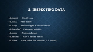
4. 2. INSPECTING DATA
• df.head() # first 5 rows
• df.tail(3) # last 3 rows
• df.info() # column types + non-null counts
• df.describe() # summary statistics
• df.shape # (rows, columns)
• df.columns # list of column names
• df.index # row index The index is 0, 1, 2 (default).

5. INDEXING, SELECTING, AND FILTERING
Column selection:
df['Name'] # single column (Series)
df[['Name', 'Score']] # multiple columns (DataFrame)

6. Row selection
df.iloc[0] # first row by position
df.iloc[0:2] # slicing by position
df.loc[1] # row with index label 1
df.loc[1:3, ['Name']] # specific rows + columns

7. • Conditional filtering
df[df['Age'] > 30] # filter rows
df[(df['Age'] > 30) & (df['Score'] > 80)] # multiple conditions

8. 4. MODIFYING DATAFRAMES
# Add new column
df['Passed'] = df['Score'] > 80
# Update values
df.loc[0, 'Score'] = 95
# Drop column
df = df.drop(columns=['Passed'])
# Rename columns
df.rename(columns={'Score': 'ExamScore'}, inplace=True)
# Change index
df.set_index('Name', inplace=True)

9. df['Score']
# 0 85.5
# 1 90.3
# 2 78.9
# 3 88.2
df['Score'] > 80
# 0 True
# 1 True
# 2 False
# 3 True
Name Age Score Passed
0 Alice 25 85.5 True
1 Bob 30 90.3 True
2 Charlie 35 78.9 False
3 David 40 88.2 True
This is how it works
df['Passed'] = df['Score'] > 80

10. DF.LOC[0, 'SCORE'] # ROW WITH INDEX=0, COLUMN='SCORE'
.loc Label-based indexing
→
• Uses row labels and column labels.
• Works with actual names (index names, column names).
.iloc Integer-location based indexing
→
• Uses row positions and column positions (like Python list indexing).
df.iloc[0, 1] # first row (0), second column (1)

11. # CHANGE INDEX
DF.SET_INDEX('NAME', INPLACE=TRUE)
Name Age Score
0 Alice 25 85
1 Bob 30 90
2 Charlie 35 78
Age Score
Name
Alice 25 85
Bob 30 90
Charlie 35 78

12. 5. HANDLING MISSING VALUES
import pandas as pd
import numpy as np
df = pd.DataFrame({
"Name": ["Alice", "Bob", "Charlie", "David"],
"Age": [25.0, np.nan, 30.0, np.nan],
"Score": [85.0, 90.0, np.nan, 70.0]
})
print(df)

13. DF.ISNULL()
Name Age Score
0 False False False
1 False True False
2 False False True
3 False True False
df.isnull().sum()
Name 0
Age 2
Score 1
dtype: int64

14. df.fillna(0) # replace NaN with 0
df.fillna(df.mean()) # replace with mean
df.dropna() # Drop rows with ANY NaN
df.dropna(axis=1) # Drop columns with ANY NaN
df.dropna(how='all') # Drop rows where ALL values are NaN
 how='any' (default) Drop the row/column if any single value is NaN.
 how=‘all 'Drop the row/column only if all values are NaN.

15. 6. GROUPING AND AGGREGATION
data = {
'Dept': ['IT', 'IT', 'HR', 'HR', 'Finance'],
'Employee': ['A', 'B', 'C', 'D', 'E'],
'Salary': [60000, 65000, 55000, 58000, 70000]
}
df = pd.DataFrame(data)
# Group by department
grouped = df.groupby('Dept')['Salary'].mean()
print(grouped)
# Multiple aggregations
df.groupby('Dept').agg({
'Salary': ['mean', 'max', 'min']
})

16. GROUPED = DF.GROUPBY('DEPT')['SALARY'].MEAN()
PRINT(GROUPED)
• import pandas as pd
• df = pd.DataFrame({
• 'Dept': ['IT', 'IT', 'HR', 'HR', 'Finance'],
• 'Employee': ['A', 'B', 'C', 'D', 'E'],
• 'Salary': [60000, 65000, 55000, 58000, 70000],
• 'Bonus': [5000, 6000, 4000, 3000, 8000]
• })
Dept
Finance 70000.0
HR 56500.0
IT 62500.0
Name: Salary, dtype:
float64

17. df.groupby('Dept').agg({
'Salary': ['mean', 'max', 'min'],
'Bonus': 'sum'
})
Salary Bonus
mean max min sum
Dept
Finance 70000.0 70000 70000 8000
HR 56500.0 58000 55000 7000
IT 62500.0 65000 60000 11000

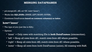
18. MERGING DATAFRAMES
• pd.merge(df1, df2, on='ID', how='inner’)
• Works like SQL JOINs (INNER, LEFT, RIGHT, OUTER).
• Combines DataFrames based on common column(s) or index.
how='inner'
• The type of join (just like in SQL).
• Options:
• 'inner' Only rows with matching IDs in
→ both DataFrames (intersection).
• 'left' Keep all rows from df1, match rows from df2 where possible.
→
• 'right' Keep all rows from df2, match rows from df1 where possible.
→
• 'outer' Keep all rows from both DataFrames (union), fill missing with NaN.
→

19. import pandas as pd
# First DataFrame
df1 = pd.DataFrame({
'ID': [1, 2, 3],
'Name': ['Alice', 'Bob', 'Charlie']
})
# Second DataFrame
df2 = pd.DataFrame({
'ID': [2, 3, 4],
'Score': [85, 90, 95]
})
# Merge
merged = pd.merge(df1, df2, on='ID', how='inner')
print(merged)
ID Name Score
0 2 Bob 85
1 3 Charlie 90

20. RESHAPING DATA
Reshaping means changing the structure or layout of DataFrame — switching
between wide and long formats, or reorganizing data for analysis.
• 1. Pivot (wide format)
• 2. Melt (long format)

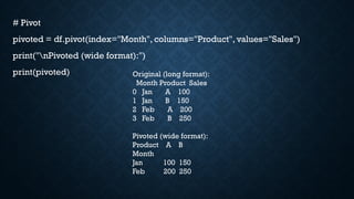
21. 1. Pivot (wide format)
Turn unique values from one column into multiple columns.
import pandas as pd
df = pd.DataFrame({
"Month": ["Jan", "Jan", "Feb", "Feb"],
"Product": ["A", "B", "A", "B"],
"Sales": [100, 150, 200, 250]
})
print("Original (long format):")
print(df)

22. # Pivot
pivoted = df.pivot(index="Month", columns="Product", values="Sales")
print("nPivoted (wide format):")
print(pivoted) Original (long format):
Month Product Sales
0 Jan A 100
1 Jan B 150
2 Feb A 200
3 Feb B 250
Pivoted (wide format):
Product A B
Month
Jan 100 150
Feb 200 250

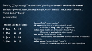
23. Melting ((Unpivoting) The reverse of pivoting — convert columns into rows.
melted = pivoted.reset_index().melt(id_vars="Month", var_name="Product",
value_name="Sales")
print(melted)
Month Product Sales
0 Jan A 10
1 Feb A 15
2 Jan B 20
3 Feb B 25
frame (DataFrame,required)
id_vars (tuple,list,or ndarray,default None)
Columns to keep fixed (not unpivoted)
value_vars (tuple,list,or ndarray,default None)
Columns to unpivot (turn into rows).
var_name (scalar, default None)
Name for the new column that will hold the old column
headers.
value_name (scalar,default "value")
Name for the new column that will hold the values.

24. • pd.melt(df, id_vars=['ID'], value_vars=['Math', 'Science'])
import pandas as pd
df = pd.DataFrame({
"ID": [1, 2, 3],
"Math": [90, 80, 85],
"Science": [88, 92, 79]
})
print(df)

25. ID Math Science
0 1 90 88
1 2 80 92
2 3 85 79
ID variable value
0 1 Math 90
1 2 Math 80
2 3 Math 85
3 1 Science 88
4 2 Science 92
5 3 Science 79
frame (DataFrame,required)
id_vars (tuple,list,or ndarray,default None)
Columns to keep fixed (not unpivoted)
value_vars (tuple,list,or ndarray,default None)
Columns to unpivot (turn into rows).
var_name (scalar, default None)
Name for the new column that will hold the old column
headers.
value_name (scalar, default "value")
Name for the new column that will hold the values.
melted = pd.melt(df, id_vars=['ID'], value_vars=['Math', 'Science'])
print(melted)

26. melted = pd.melt(
df,
id_vars=["Student"],
value_vars=["Math", "Science",
"English"],
var_name="Subject",
value_name="Marks"
)
print(melted)
Student Math Science English
0 A 90 88 95
1 B 80 92 85
2 C 85 79 87

27. melted = pd.melt(
df,
id_vars=["Student"],
value_vars=["Math", "Science", "English"],
var_name="Subject",
value_name="Marks"
)
print(melted)
Student Subject Marks
0 A Math 90
1 B Math 80
2 C Math 85
3 A Science 88
4 B Science 92
5 C Science 79
6 A English 95
7 B English 85
8 C English 87

28. 3. STACK / UNSTACK
Stack: moves columns into the row index.Unstack: moves
row index levels into columns.
stacked = pivoted.stack()
print(stacked)
Month Product
Jan A 10
B 20
Feb A 15
B 25
dtype: int64

29. unstacked = stacked.unstack()
print(unstacked) Product A B
Month
Jan 10 20
Feb 15 25

30. 4. TRANSPOSE (.T)
Flip rows and columns.
print(df.T)

31. DATA WRANGLING
Data wrangling (or data munging) in pandas means cleaning, reshaping,
transforming, and enriching raw data into a usable format for analysis or modeling.
Load & Inspect
CleanTransform
Reshape
Filter & Subset
Aggregate & Summarize
Combine Data
Reindex & Sor
tFeature Engineering