![BASIC DEFINITIONS [1]
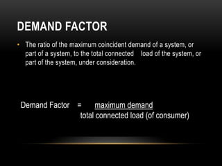
Load
The power consumed by a Electrical Circuit.
Forecasting
The process of making statements about events
whose actual outcomes have not yet been observed.
Load forecasting
An estimate of power demand at some future period.](https://image.slidesharecdn.com/group-7loadforecastingharmonicsfinalppt-120629071245-phpapp02/85/Group-7-load-forecasting-harmonics-final-ppt-3-320.jpg)


![[7]](https://image.slidesharecdn.com/group-7loadforecastingharmonicsfinalppt-120629071245-phpapp02/85/Group-7-load-forecasting-harmonics-final-ppt-13-320.jpg)


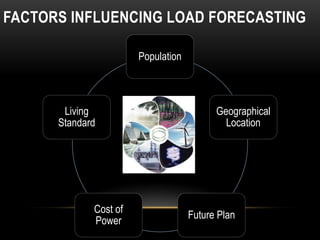
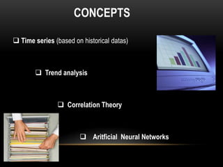
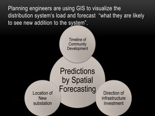
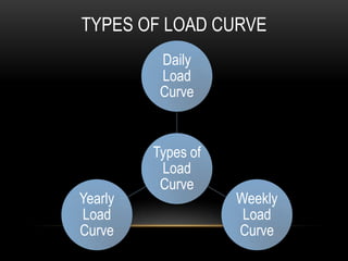
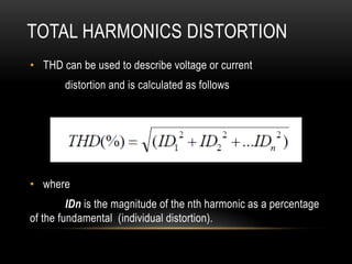
![Type of Demand Load Utilization
Industry Factor Factor Factor
Induction furnace 0.99 0.80 0.72
Steel Rolling Mills 0.80 0.25 0.72
Textile Industry 0.50 0.80 0.40
Gas Plant Industry 0.70 0.50 0.35
College & Schools 0.50 0.20 0.10
Paper Industry 0.50 0.80 0.40
Source[Electrical engineering portal]](https://image.slidesharecdn.com/group-7loadforecastingharmonicsfinalppt-120629071245-phpapp02/85/Group-7-load-forecasting-harmonics-final-ppt-25-320.jpg)
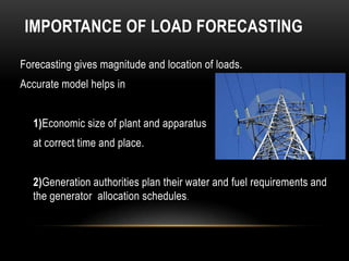
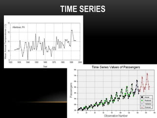
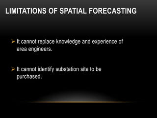
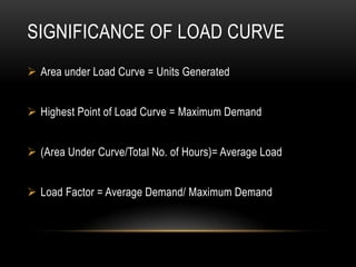
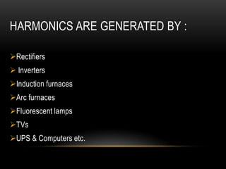
![DEMAND SUPPLY FORECAST : INDIA
[5]](https://image.slidesharecdn.com/group-7loadforecastingharmonicsfinalppt-120629071245-phpapp02/85/Group-7-load-forecasting-harmonics-final-ppt-27-320.jpg)


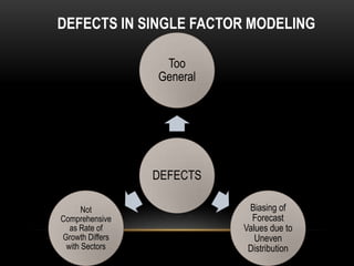
![SINGLE FACTOR MODELING [2]
Single factor modeling is based on a model that
assumes one dominant factor, determines the
model outcome.](https://image.slidesharecdn.com/group-7loadforecastingharmonicsfinalppt-120629071245-phpapp02/85/Group-7-load-forecasting-harmonics-final-ppt-48-320.jpg)


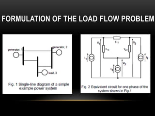
![FORMULATION OF THE LOAD FLOW PROBLEM
where [Y] is the nodal admittance matrix](https://image.slidesharecdn.com/group-7loadforecastingharmonicsfinalppt-120629071245-phpapp02/85/Group-7-load-forecasting-harmonics-final-ppt-65-320.jpg)


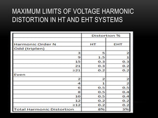
![PROPAGATION OF HARMONICS IN THE NETWORK
INFLUENCE OF PHASE ANGLE OF HARMONICS[6]](https://image.slidesharecdn.com/group-7loadforecastingharmonicsfinalppt-120629071245-phpapp02/85/Group-7-load-forecasting-harmonics-final-ppt-75-320.jpg)


![REFERENCES
• [1].International Journal of Systems Science, volume
33, number 1.
• [2]. Electrical engineering portal
• [3].US electric static schneider
• [4].Department of Electrical and Electronics Engineering, S.V.U.
College of Engineering, Tirupati, A.P., India
• [5].India Energy Handbook.
• [6] Dept. of Electrical,Electronic and Control
Engineering, Ciudad Universitaria. Madrid. Spain.
• [7] NRLDC.nic.in](https://image.slidesharecdn.com/group-7loadforecastingharmonicsfinalppt-120629071245-phpapp02/85/Group-7-load-forecasting-harmonics-final-ppt-89-320.jpg)


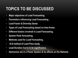
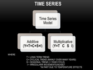
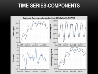
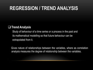
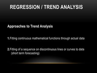
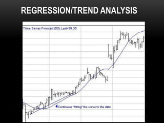
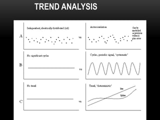
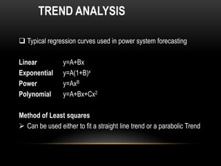
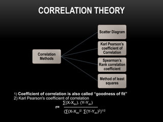
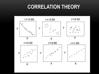
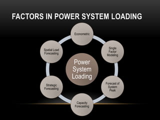
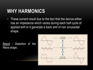
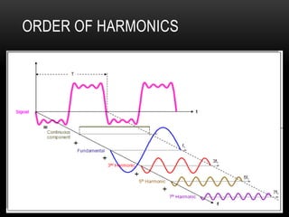
1) The document discusses load forecasting, including the objectives, factors influencing it, and types based on time frame. 2) Key factors in load forecasting include population, living standards, geographical location, cost of power, weather, time of day, and customer class. Accurate load forecasting helps utilities with generation planning and infrastructure development. 3) The document covers various load forecasting methods including time series analysis, regression/trend analysis, and correlation theory. Time series models include additive and multiplicative models, while regression analyzes trends using linear, exponential, power, and polynomial curves.


![Power system planning & operation [eceg 4410]](https://cdn.slidesharecdn.com/ss_thumbnails/powersystemplanningoperationeceg-4410-130607134359-phpapp01-thumbnail.jpg?width=640&height=640&fit=bounds)