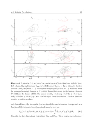
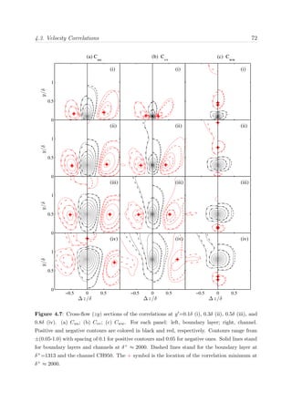
Download to read offline


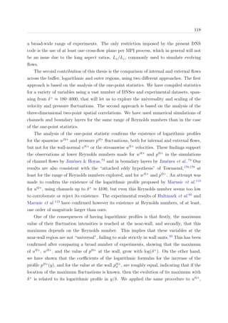
![2.4. The numerical code 19
planetopencil
penciltoplane
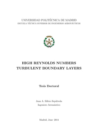
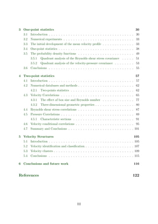
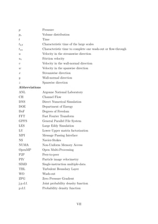
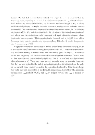
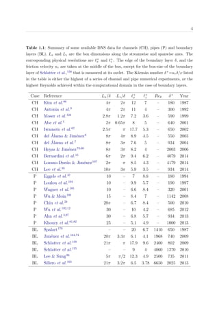
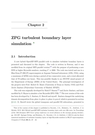
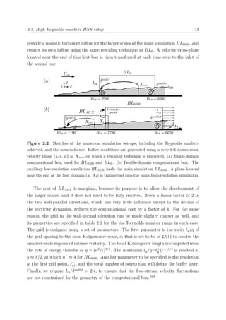
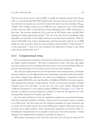
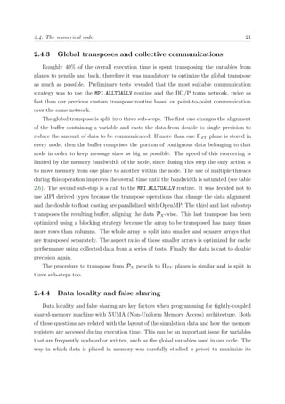
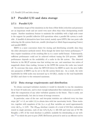
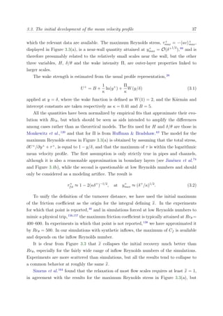
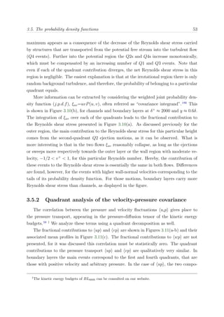
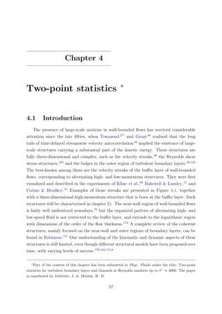
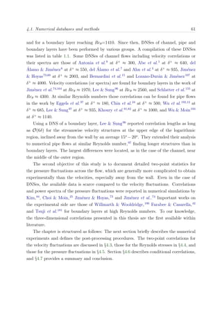
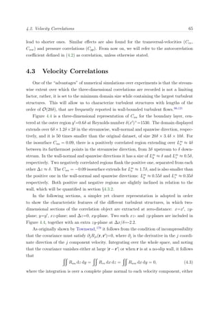
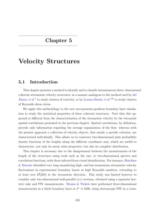
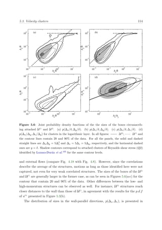
Figure 2.4: Partition of the computational domain for OpenMP-MPI for N nodes and four
threads. Top, ΠZY planes; bottom, PX pencil
The different MPI tasks are mapped to the nodes, and OpenMP is applied within each of
those nodes, splitting the sub-domain in a number of pieces equal to the available number
of threads, four in BG/P, in which each individual thread is mapped to a physical core.
The variables are most of the time allocated in memory as ψ(Nk, Ny, Nx/N ), where
Nk is the number of dealiased Fourier modes in the spanwise direction (2/3Nz). Each
thread works in the same memory region of the shared variables using a first-touch data
placement policy,111
maximizing the data locality and diminishing the cache missed,131
thus improving the overall performance of the code.
The most common configuration that a team of threads can find is presented in Fig-
ure 2.4, in which each thread works over a portion of size [Nk(Nx/N )]Ny/Nthreads with
static scheduling along the wall-normal index, where Nthread is the total number of threads.
This scheduling is defined manually through thread private indexes, which maximizes
memory reuse. A more detailed discussion is offered in section §2.4.4. In that way, each
thread always works in the same portion of the array. Nevertheless, when loop depen-
dencies are found in the wall-normal direction, for instance in the resolution of the LU
linear system of equations, threads work over portions of Nk instead. For such loops,
blocking techniques are used, putting the innermost loop index to the outermost part,
which maximize data locality since strips of the arrays fit into the cache at the same time
that threads can efficiently share the work load. The block size was manually tuned for](https://image.slidesharecdn.com/c925b986-f353-4026-9444-b6b91a9160be-160513220740/85/thesis_sillero-36-320.jpg)
![2.5. Blue Gene/P mapping 23
coordinates [X, Y, Z]. Different physical layouts of MPI tasks onto physical processors are
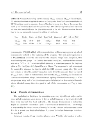
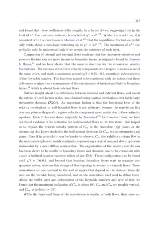
predefined depending on the number of nodes to be allocated. The predefined mapping
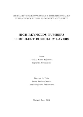
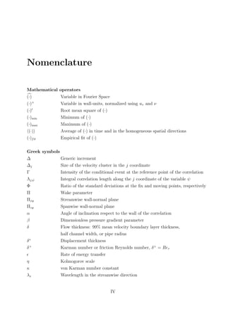
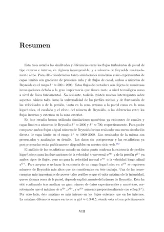
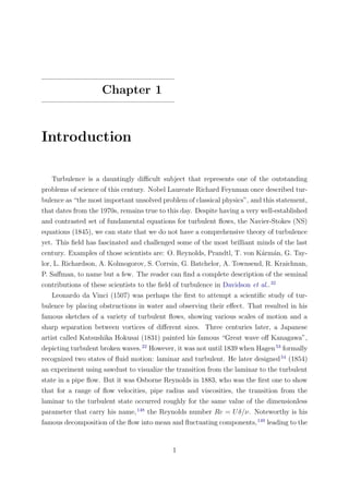
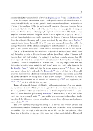
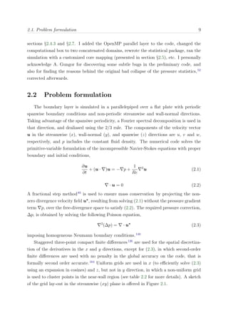
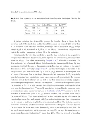
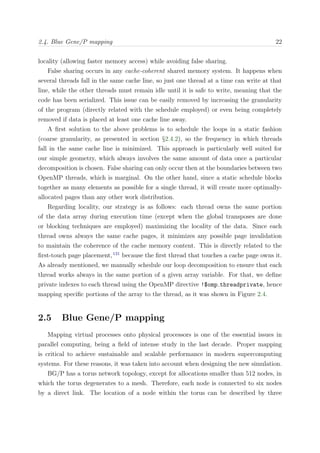
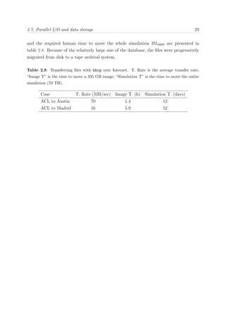
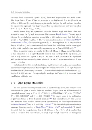
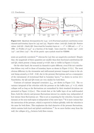
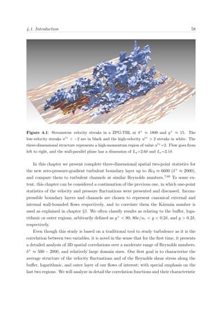
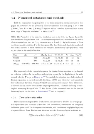
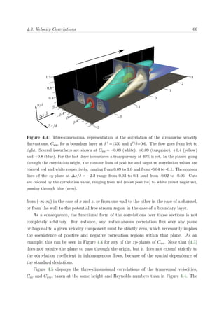
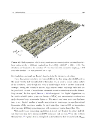
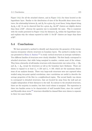
for a 512 node partition is a [8, 8, 8] topology, while for 8192 nodes it is [8, 32, 32], as shown
in Figure 2.5. Users can specify their desired node topology by using the environment
variable BG MAPPING and specifying the topology in a plain text file.
Figure 2.5: Predefined (left) and custom (right) node mapping for a 8192 node partition in a
[8, 32, 32] topology. The predefined mapping assigns to BLAUX (BL1) the nodes in a [8, 32, 2]
sub-domain. Custom mapping assigns the nodes to a [8, 8, 8] sub-domain. BL6600 is mapped to
the rest of the domain till complete the partition. Symbol • stand for an arbitrary node, and
(red) • for a neighbor node connected by a direct link.
Changing the node topology completely changes the graph embedding problem and
the path in which the MPI message travels. This can increase or decrease the number of
hops (i.e. one portion of the path between source and destination) needed to connect one
node to another, and as a result, alters the communication time to send a message. Fine
tuning for specific problems can considerably improve the time spent in communications.
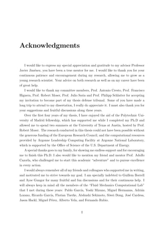
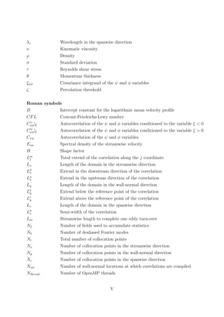
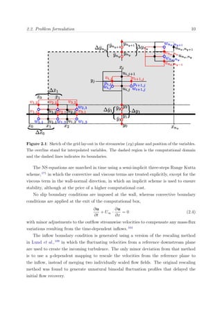
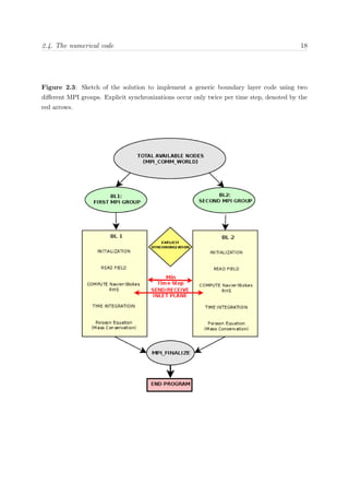
Table 2.5 shows different mappings that were tested for our specific problem size. Our
custom mapping reduces the communication time for BLAUX by a factor of 2. The work
load for BLAUX is projected using this new communication time, whereas the load for
BL6600 is fixed as already mentioned. Balance is achieved minimizing the time in which
either BLAUX or BL6600 are idle during execution time.
The choice of a user-defined mapping was motivated due to the particular distribution
of nodes and MPI groups. The first boundary layer BLAUX runs in 512 MPI processes
mapped onto the first 512 nodes, while BL6600 runs in 7680 MPI processes mapped on the
remaining nodes, ranging from 513 to 8192. Note that at the moment that the communi-
cator (denoted as C) is split such that CBLAUX
∪ CBL6600 =MPI COMM WORLD, neither CBLAUX
nor CBL6600 can be on a 3D torus network anymore. As a consequence, the communication](https://image.slidesharecdn.com/c925b986-f353-4026-9444-b6b91a9160be-160513220740/85/thesis_sillero-40-320.jpg)
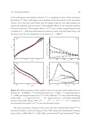
![2.5. Scalability results in Blue Gene/P 24
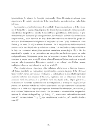
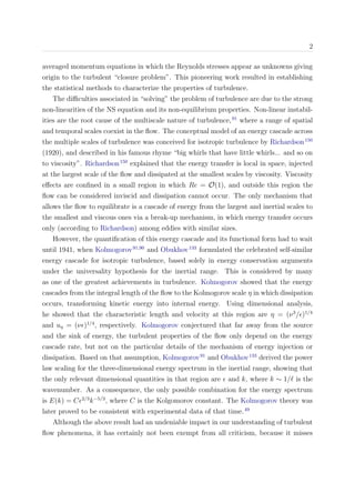
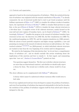
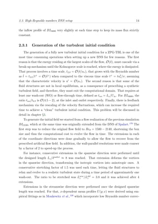
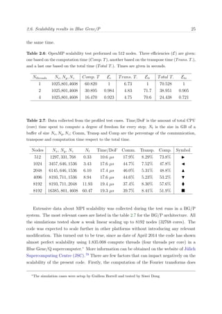
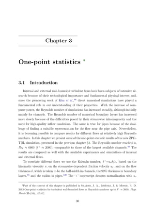
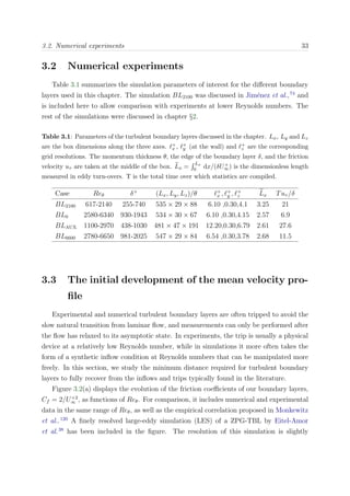
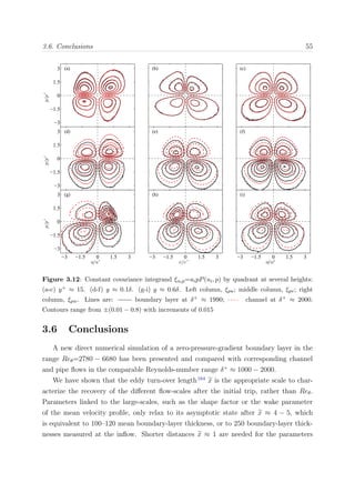
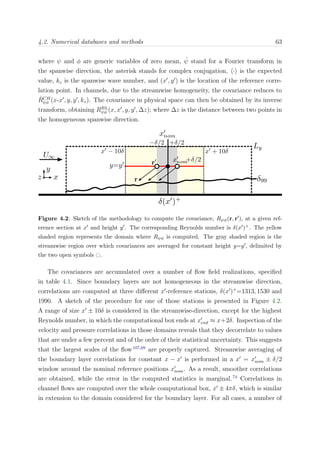
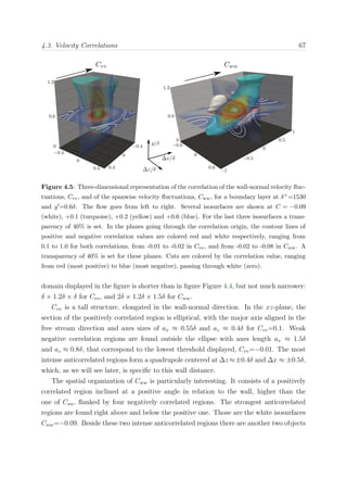
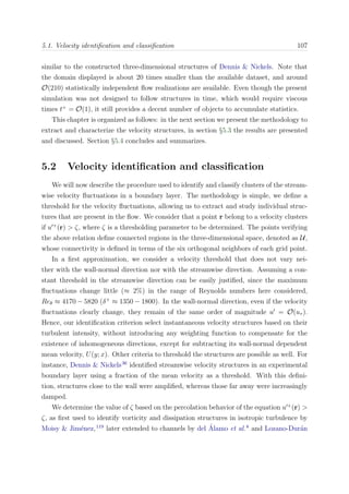
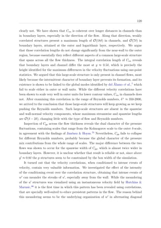
Table 2.5: Time spent in communication during global transposes. Different node topologies
are presented for 10 time steps and for each boundary layer. Times are given in seconds.
Case Topology Nodes Comm BLAUX Comm BL6600
Predefined [8, 8, 8] 512 27.77 —
Predefined [8, 32, 32] 8192 160.22 85.44
Custom [8, 32, 32] 8192 79.59 86.09
will take place within a 2D mesh with sub-optimal performance. The optimum topology
for our particular problem would be the one in which the number of hops within each
MPI group is minimum, since collective communications occur locally for each group.
For a single 512 node partition the optimum is the use of a [8, 8, 8] topology, in which
the MPI messages travel within a single communication switch. We found that a better
mapping for BLAUX was a [8, 8, 8] sub-domain within the predefined [8, 32, 32] domain, as
shown in the right side of Figure 2.4. BL6600 is mapped to the remaining nodes using the
predefined topology. No other mappings were further investigated.
Note that a [8, 8, 8] topology was used in analogy to the single 512 node partition and
the measured communication time found is substantially greater. The reason is that the
512 node partition (named midplane) is a special case having a different type of network,
a global collective tree.4
This network is characterized by presenting a higher-bandwidth
for global collective operations than the 3D-torus network, which explains the profiling
time obtained.
The methodology to optimize communications for other partition sizes would be similar
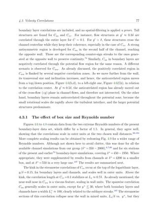
to the one just described: mapping virtual processes to nodes that are physically as close
as possible, thus minimizing the number of hops.
2.6 Scalability results in Blue Gene/P
Some tests were run in a 512 node configuration after porting the code to OpenMP.
The results are shown in table 2.6. These samples suggest that almost no penalty is paid
when the computations are parallelized with OpenMP. In addition, the problem size per
node and the MPI message size can be increased by a factor of 4 while using all the
resources at node level. The efficiency of the transposes is relatively low due to memory
contention, since two or more threads try to read items in the same block of memory at](https://image.slidesharecdn.com/c925b986-f353-4026-9444-b6b91a9160be-160513220740/85/thesis_sillero-41-320.jpg)

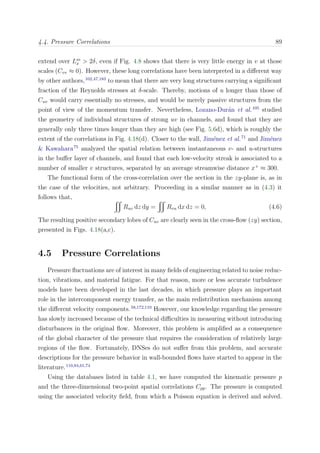
![3.1. Introduction 31
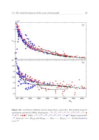
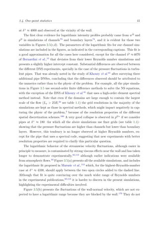
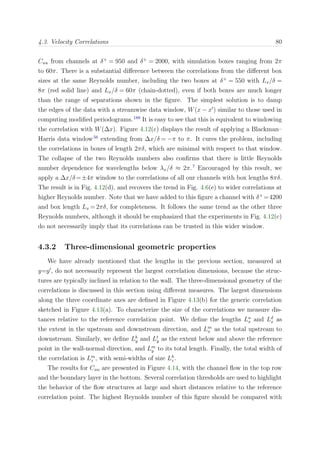
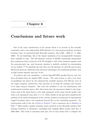
and ν. The Reynolds number Reθ = U∞θ/ν is defined for boundary layers in terms of
the momentum thickness θ and of the free-stream velocity U∞.
Our first goal is to characterize the initial development of the velocity statistics in
experimentally or numerically tripped boundary layers. In the careful study by Erm &
Joubert40
of the effect of different experimental tripping devices, the authors conclude
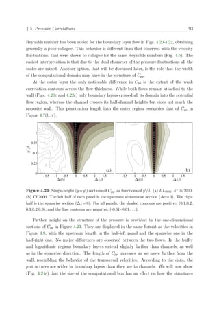
that the differences observed in the mean velocity profile disappear beyond Reθ ≈ 3000.
Likewise, Schlatter & ¨Orl¨u157
analyze the effect of different low-Reynolds-number trips
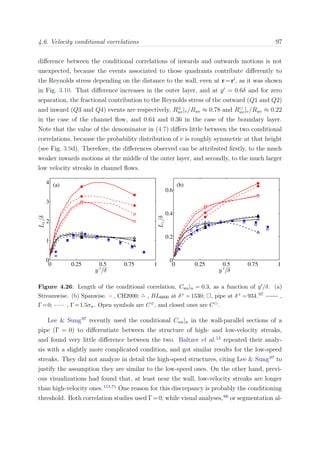
on their DNS statistics, and show that a well-established boundary layer is attained at
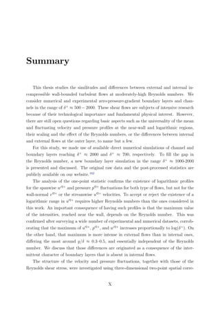
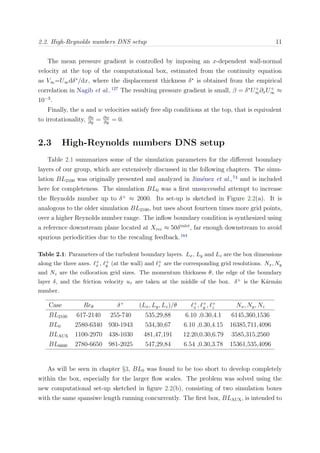
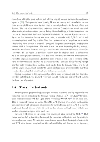
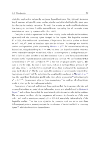
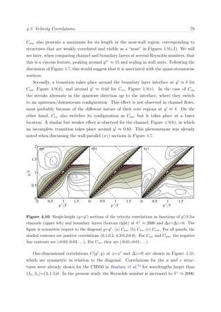
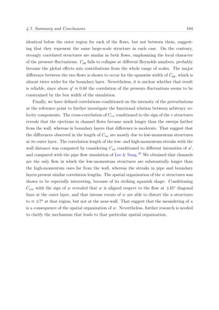
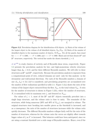
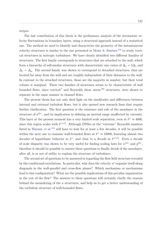
Reθ ≈ 2000. On the other hand, Simens et al.164
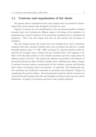
proposed that the turnover length,
defined as the distance Lto = U∞δ/uτ by which eddies are advected during a turnover
time δ/uτ , provides a better description than the Reynolds number of how fast boundary
layer simulations recover from synthetic inflow conditions. They found that at least one
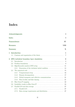
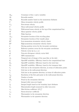
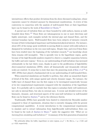
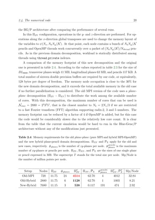
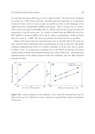
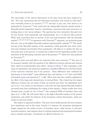
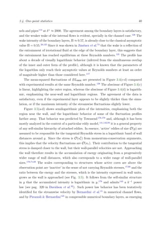
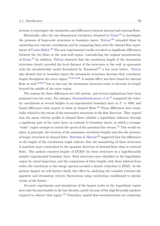
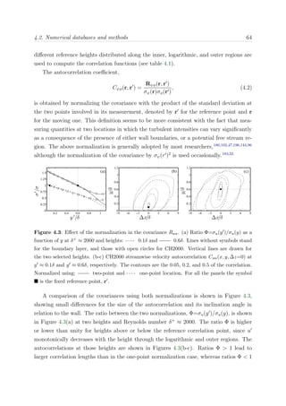
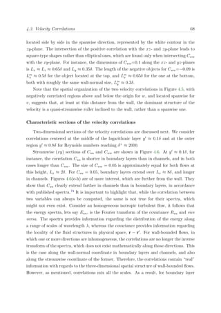
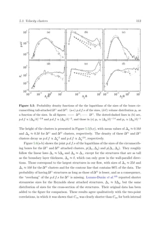
eddy-turnover is required for most flow scales to decorrelate from the inlet. Figure 3.1
shows an estimate of the integrated turn-over distance with the Reynolds number Reθ,
based on the empirical correlations proposed in Nagib et al.,127
for each of the boundary
layers of our group.
0 1000 2000 3000 4000 5000 6000 7000 8000
1
3
5
7
9
Re
θ
∫u
τ
/δ
99
U
∞
dx
Figure 3.1: Integral turn-over length x =
x
[ dx/(δU+
∞)] as a function of the Reynolds number
Reθ for the different boundary layers cases. Symbols are: • BL2100, BL0, BLAUX, and
BL6600.
Using the new data, we will compare the relative merits of the Reynolds number and
of the turnover length as indicators of recovery, and we will show that the recovery length
of the largest scales is considerable longer than the decorrelation length mentioned above.
Our second goal is to examine the universality of the mean and fluctuating velocity
profiles in the near-wall and logarithmic regions, and to inquire on the similarities and
differences between internal (channels and pipes) and external (boundary layers) flows.](https://image.slidesharecdn.com/c925b986-f353-4026-9444-b6b91a9160be-160513220740/85/thesis_sillero-48-320.jpg)

![References
[1] Abe, H., Kawamura, H. & Matsuo, Y. 2001 Direct numerical simulation of fully developed
turbulent channel flow with respect to the Reynolds number dependence. J. Fluids Eng. 123, 382
– 393.
[2] Adrian, R. J., Meinhart, C. D. & Tomkins, C. D. 2000 Vortex organization in the outer
region of the turbulent boundary layer. J. Fluid Mech. 422, 1–53.
[3] Ahn, Junsun, Lee, Jae Hwa, Jang, Sung Jae & Sung, Hyung Jin 2013 Direct numerical
simulations of fully developed turbulent pipe flows for Reτ =180, 544 and 934. Int. Journal of Heat
and Fluid Flow 44 (0), 222 – 228.
[4] Alam, S., Barrett, R., Bast, M., Fahey, M. R., Kuehn, J., McCurdy, C., Rogers, J.,
Roth, P., Sankaran, R., Vetter, J. S., Worley, P. & Yu, W. 2008 Early evaluation of
IBM BlueGene/P. SC Conference 0, 1–12.
[5] del Alamo, J.C. & Jim´enez, J. 2009 Estimation of turbulent convection velocities and correc-
tions to Taylor’s approximation. J. Fluid Mech. 640, 5–26.
[6] del ´Alamo, J. C. & Jim´enez, J. 2003 Spectra of the very large anisotropic scales in turbulent
channels. Phys. Fluids 15 (6), L41–L44.
[7] del ´Alamo, J. C., Jim´enez, J., Zandonade, P. & Moser, R. D. 2004 Scaling of the energy
spectra of turbulent channels. J. Fluid Mech. 500, 135–144.
[8] del ´Alamo, J. C., Jim´enez, J., Zandonade, P. & Moser, R. D. 2006 Self-similar vortex
clusters in the turbulent logarithmic region. J. Fluid Mech. 561, 329–358.
[9] Antonia, R. A., Teitel, M., Kim, J. & Browne, L. W. B. 1992 Low-Reynolds-number effects
in a fully developed turbulent channel flow. J. Fluid. Mech. 236, 579–605.
[10] Bailey, S. C. C. & Smits, A. J. 2010 Experimental investigation of the structure of large- and
very-large-scale motions in turbulent pipe flow. J. Fluid Mech. 651, 339–356.
[11] Bakewell, H. P. & Lumley, J. L. 1967 Viscous Sublayer and Adjacent Wall Region in Turbulent
Pipe Flow. Phys. Fluids 10 (9), 1880–1889.
[12] Baltzer, J. R., Adrian, R. J. & Wu, X. 2013 Structural organization of large and very large
scales in turbulent pipe flow simulation. J. Fluid Mech. 720, 236–279.
[13] Barenblatt, G. I. & Chorin, A. J. 1998 New perspectives in turbulence: scaling laws, asymp-
totics and intermittency. SIAM Rev. 40, 265 – 291.
[14] Batchelor, G. K. 1953 The theory of homogeneous turbulence. Cambridge U. Press.
[15] Bernardini, M., Pirozzoli, S. & Orlandi, P. 2014 Velocity statistics in turbulent channel
flow up to Reτ = 4000. J. Fluid Mech. 742, 171–191.
[16] Borrell, G., Sillero, J.A. & Jim´enez, J. 2013 A code for direct numerical simulation of
122](https://image.slidesharecdn.com/c925b986-f353-4026-9444-b6b91a9160be-160513220740/85/thesis_sillero-139-320.jpg)
![123
turbulent boundary layers at high Reynolds numbers in BG/P supercomputers. Computers & Fluids
80 (0), 37 – 43.
[17] Bradshaw, P. 1967 Irrotational fluctuations near a turbulent boundary layer. J. Fluid Mech. 27,
209–230.
[18] Brown, G.L. & Roshko, A. 1974 On the density effects and large structure in turbulent mixing
layers. J. Fluid Mech. 64, 775 – 816.
[19] Bull, M.K. & Thomas, A.S.W. 1976 High frequency wall-pressure fluctuations in turbulent
boundary layers. Phys. Fluids 19 (4), 597–599.
[20] Bullock, K. J., Cooper, R. E. & Abernathy, F. H. 1978 Structural similarity in radial
correlations and spectra of longitudinal velocity fluctuations in pipe flow. J. Fluid Mech. 88, 585–
608.
[21] Buschmann, M.H. & Gad-el-Hak, M. 2010 Normal and cross-flow Reynolds stresses: differences
between confined and semi-confined flows. Experiments in Fluids 49 (1), 213–223.
[22] Cartwright, J. H. E. & Nakamura, H. 2009 What kind of a wave is Hokusais Great wave off
Kanagawa? Notes and Records of the Royal Society 63 (2), 119–135.
[23] Chevalier, M., Schlatter, P., Lundbladh, A. & Henningson, D.S. 2007 Simson - a pseudo-
spectral solver for incompressible boundary layer flows. Tech. Rep.. TRITA-MEK 2007:07.
[24] Chin, C., Ooi, A. S. H., Marusic, I. & Blackburn, H. M. 2010 The influence of pipe length
on turbulence statistics computed from direct numerical simulation data. Phys. Fluids 22 (11), –.
[25] Choi, H. & Moin, P. 1990 On the space-time characteristics of wall-pressure fluctuations. Phys.
Fluids A 2, 1450–1460.
[26] Christensen, K. T. 2001 Experimental investigation of acceleration and velocity fields in turbu-
lent channel flow. PhD thesis, University of Illinois at Urbana-Champaign.
[27] Clauser, F.H. 1956 The turbulent boundary layer. Advances in Applied Mechanics 4.
[28] Coles, D.E. 1956 The law of the wake in the turbulent boundary layer. J. Fluid Mech. 1 (02),
191–226.
[29] Coles, D.E. 1968 The young people’s guide to the data. In Proceedings Computation of Turbulent
Boundary Layers. Stanford Univ., , vol. 2, pp. 1–19. D.E. Coles and E.A. Hirst.
[30] Comte-Bellot, G. 1965 ´Ecoulement turbulent entre deux parois parell`eles. Pub. Scientifiques
Techniques 419. Minist`ere de L’Air.
[31] Corino, E. R. & Brodkey, R. S. 1969 A visual investigation of the wall region in turbulent
flow. J. Fluid Mech. 37, 1–30.
[32] Davidson, P.A., Kaneda, Y., Moffatt, K. & Sreenivasan, K.R. 2011 A Voyage Through
Turbulence. Cambridge University Press.
[33] De Graaf, D.B. & Eaton, J.K. 2000 Reynolds number scaling of the flat-plate turbulent bound-
ary layer. J. Fluid Mech. 422, 319–346.
[34] Delo, C. J., Kelso, R. M. & Smits, A. J. 2004 Three-dimensional structure of a low-Reynolds-
number turbulent boundary layer. J. Fluid. Mech. 512, 47–83.
[35] Dennis, D. J. C. & Nickels, T. B. 2011 Experimental measurement of large-scale three-
dimensional structures in a turbulent boundary layer. Part 1. Vortex packets. J. Fluid Mech. 673,
180–217.
[36] Dennis, D. J. C. & Nickels, T. B. 2011 Experimental measurement of large-scale three-](https://image.slidesharecdn.com/c925b986-f353-4026-9444-b6b91a9160be-160513220740/85/thesis_sillero-140-320.jpg)
![124
dimensional structures in a turbulent boundary layer. Part 2. Long structures. J. Fluid Mech.
673, 218–244.
[37] Eggels, J. G. M., Unger, F., Weiss, M. H., Westerweel, J., Adrian, R. J., Friedrich,
R. & Nieuwstadt, F. T. M. 1994 Fully developed turbulent pipe flow: a comparison between
direct numerical simulation and experiment. J. Fluid Mech. 268, 175 – 209.
[38] Eitel-Amor, Georg, ¨Orl¨u, Ramis & Schlatter, Philipp 2014 Simulation and validation of
a spatially evolving turbulent boundary layer up to Reθ = 8300. Int. Journal of Heat and Fluid
Flow 47 (0), 57 – 69.
[39] Elsinga, G.E. & Marusic, I. 2010 Evolution and lifetimes of flow topology in a turbulent
boundary layer. Phys. Fluids 22 (1), –.
[40] Erm, L.P. & Joubert, P.N. 1991 Low-Reynolds-number turbulent boundary layers. J. Fluid
Mech. 230, 1–44.
[41] Farabee, T.M. & Casarella, M.J. 1986 Measurements of fluctuating wall pressure for sepa-
rated/reattached boundary layer flows. Journal of Vibration, Acoustics, Stress and Reliability in
Design 108, 301–307.
[42] Farabee, T.M. & Casarella, M.J. 1991 Spectral features of wall pressure fluctuations beneath
turbulent boundary layers. Phys. Fluids 3, 2410–2419.
[43] Favre, A. J., Gaviglio, J. J. & Dumas, R. 1957 Space-time double correlations and spectra in
a turbulent boundary layer. J. Fluid Mech. 2, 313–342.
[44] Ferrante, A. & Elghobashi, S. 2005 Reynolds number effect on drag reduction in a
microbubble-laden spatially developing turbulent boundary layer. J. Fluid Mech. 543, 93–106.
[45] Flores, O. & Jim´enez, J. 2010 Hierarchy of minimal flow units in the logarithmic layer. Phys.
Fluids 22, 071704.
[46] Frings, Wolfgang, Wolf, Felix & Petkov, Ventsislav 2009 Scalable Massively Parallel I/O
to Task-local Files. In Proceedings of the Conference on High Performance Computing Networking,
Storage and Analysis, pp. 17:1–17:11. New York, NY, USA: ACM.
[47] Ganapathisubramani, B., Hutchins, N., Hambleton, W. T., Longmire, E. K. & Maru-
sic, I. 2005 Investigation of large-scale coherence in a turbulent boundary layer using two-point
correlations. J. Fluid Mech. 524, 57–80.
[48] Grant, H. L. 1958 The large eddies of turbulent motion. J. Fluid Mech. 4, 149–190.
[49] Grant, H. L., Stewart, R. W. & Moilliet, A. 1962 Turbulence spectra from a tidal channel.
J. Fluid. Mech. 12, 241 – 268.
[50] Gropp, W., Lusk, E. & Skjellum, A. 1999 Using MPI (2Nd Ed.): Portable Parallel Program-
ming with the Message-passing Interface. Cambridge, MA, USA: MIT Press.
[51] Guala, M., Hommema, S. E. & Adrian, R. J. 2006 Large-scale and very-large-scale motions
in turbulent pipe flow. J. Fluid Mech. 554, 521–542.
[52] Gungor, A.G., Sillero, J.A. & Jim´enez, J. 2012 Pressure statistics from direct simulation
of turbulent boundary layer. In Proceedings of the 7th International Conference on Computational
Fluid Dynamics, pp. 1–6.
[53] Hagen, G. 1839 ¨Uber die Bewegung des Wassers in engen cylindrischen R¨ohren. Annalen der
Physik 122 (3), 423–442.
[54] H¨agen, G. 1854 ¨Uber den einfluss der temperatur auf die bewegung des wassers in R¨ohren. Math.](https://image.slidesharecdn.com/c925b986-f353-4026-9444-b6b91a9160be-160513220740/85/thesis_sillero-141-320.jpg)
![125
Abh. Akad. Wiss Berlin 17, 17 – 98.
[55] Hanushevsky, A. 2008 BBCP. http://www.slac.stanford.edu/~abh/bbcp/.
[56] Harris, F.J. 1978 On the use of windows for harmonic analysis with the discrete fourier transform.
Proc. IEEE 66 (1), 51–83.
[57] Head, M. R. & Bandyopadhyay, P. 1981 New aspects of turbulent boundary-layer structure.
J. Fluid Mech. 107, 297–338.
[58] Hinze, J.O. 1975 Turbulence, 2nd edn. McGraw-Hill.
[59] Hites, M. 1997 Scaling of high-Reynolds number turbulent boundary layers in the national diag-
nostic facility. Ph.D. thesis, Illinois Inst. of Technology.
[60] Hoyas, S. & Jim´enez, J. 2006 Scaling of the velocity fluctuations in turbulent channels up to
Reτ = 2003. Phys. Fluids 18, 011702.
[61] Hoyas, S. & Jim´enez, J. 2008 Reynolds number effects on the Reynolds-stress budgets in turbu-
lent channels. Phys. Fluids 20 (10), 101511.
[62] Hu, Z.W., Morfey, C.L. & Sandham, N.D. 2006 Wall pressure and shear stress spectra from
direct simulations of channel flow. AIAA J. 44 (7), 1541–1549.
[63] Huffman, G.D. & Bradshaw, P. 1972 A note on von K´arm´an’s constant in low Reynolds number
turbulent flows. J. Fluid Mech. 53, 45–60.
[64] Hultmark, M., Bailey, S.C.C & Smits, A.J. 2010 Scaling of near-wall turbulence in pipe flow.
J. Fluid Mech. 649, 103–113.
[65] Hultmark, M., Vallikivi, M., Bailey, S. C. C. & Smits, A. J. 2012 Turbulent pipe flow at
extreme Reynolds numbers. Phys. Rev. Lett. 108, 094501.
[66] Hutchins, N. & Marusic, I. 2007 Evidence of very long meandering features in the logarithmic
region of turbulent boundary layers. J. Fluid Mech. 579, 467–477.
[67] Iwamoto, K., Suzuki, Y. & Kasagi, N. 2002 Reynolds number effect on wall turbulence: toward
effective feedback control. Int. Journal of Heat and Fluid Flow 23 (5), 678 – 689.
[68] Jim´enez, J. 1998 The largest scales of turbulence. In CTR Ann. Res. Briefs, pp. 137–154. Stanford
Univ.
[69] Jim´enez, J. 2012 Cascades in wall-bounded turbulence. Ann. Rev. Fluid Mech. 44, 27–45.
[70] Jim´enez, J. 2013 Near-wall turbulence. Phys. Fluids 25 (10), –.
[71] Jim´enez, J., del ´Alamo, J. C. & Flores, O 2004 The large-scale dynamics of near-wall
turbulence. J. Fluid Mech. 505, 179–199.
[72] Jim´enez, J. & Garc´ıa-Mayoral, R. 2011 Direct simulations of wall-bounded turbulence. In
Direct and Large-Eddy Simulation VIII (ed. H. Kuerten, B. Geurts, V. Armenio & J. Fr¨ohlich),
pp. 3–8. Springer Netherlands.
[73] Jim´enez, J. & Hoyas, S. 2008 Turbulent fluctuations above the buffer layer of wall-bounded
flows. J. Fluid Mech. 611, 215–236.
[74] Jim´enez, J., Hoyas, S., Simens, M.P. & Mizuno, Y. 2010 Turbulent boundary layers and
channels at moderate Reynolds numbers. J. Fluid Mech. 657, 335–360.
[75] Jim´enez, J & Kawahara, G 2013 Ten Chapters in Turbulence, chap. Dynamics of Wall-Bounded
Turbulence. Cambridge University Press.
[76] Jim´enez, J & Lozano-Dur´an, A. 2014 Progress in Wall Turbulence: Understanding and Mod-
eling, chap. Coherent structures in wall-bounded turbulence. Springer, (To appear).](https://image.slidesharecdn.com/c925b986-f353-4026-9444-b6b91a9160be-160513220740/85/thesis_sillero-142-320.jpg)
![126
[77] Jim´enez, J. & Moser, R.D. 2007 What are we learning from simulating wall turbulence? Phil.
Trans. R. Soc. A 365, 715–732.
[78] Jim´enez, Javier & Pinelli, Alfredo 1999 The autonomous cycle of near-wall turbulence. J
Fluid Mech 389, 335–359.
[79] J¨ulich Supercomputing Centre (JSC) 2014 High-Q Club: Highest Scaling Codes on Juqueen.
http://fz-juelich.de/ias/jsc/EN/Expertise/High-Q-Club/OpenTBL/_node.html.
[80] von K´arm´an, T. 1930 Mechanische Ahnlichkeit und turbulenz. In Proceedings Third Int. Congr.
Applied Mechanics, Stockholm, pp. 85–105.
[81] Khoury, George., Schlatter, Philipp, Noorani, Azad, Fischer, Paul., Brethouwer,
Geert & Johansson, Arne. 2013 Direct Numerical Simulation of Turbulent Pipe Flow at Mod-
erately High Reynolds Numbers. Flow, Turbulence and Combustion 91 (3), 475–495.
[82] Khoury, George K El, Schlatter, Philipp, Brethouwer, Geert & Johansson, Arne V
2014 Turbulent pipe flow: Statistics, Re-dependence, structures and similarities with channel and
boundary layer flows. Journal of Physics: Conference Series 506 (1), 012010.
[83] Khujadze, G. & Oberlack, M. 2004 DNS and scaling laws from new symmetry groups of ZPG
turbulent boundary layer flow. Theoretical and Computational Fluid Dynamics 18 (5), 391–411.
[84] Kim, J. 1989 On the structure of pressure fluctuations in simulated turbulent channel flow. J. Fluid
Mech. 205, 421–451.
[85] Kim, J. & Moin, P. 1985 Application of a fractional-step method to incompressible Navier-Stokes
equations. J. Comput. Phys. 59 (2), 308–323.
[86] Kim, J., Moin, P. & Moser, R. D. 1987 Turbulence statistics in fully developed channel flow
at low Reynolds number. J. Fluid Mech. 177, 133–166.
[87] Kim, K. & Adrian, R. J. 1999 Very large-scale motion in the outer layer. Phys. Fluids 11,
417–422.
[88] Klewicki, J.C., Fife, P., Wei, T. & McMurtry, P. 2007 A physical model of the turbulent
boundary layer consonant with mean momentum balance structure. Phil. Trans. Roy. Soc A 365,
823–839.
[89] Kline, S. J., Reynolds, W. C., Schraub, F. A. & Runstadler, P. W. 1967 The structure
of turbulent boundary layers. J. Fluid Mech. 30, 741–773.
[90] Kolmogorov, A. N. 1941 Dissipation of energy in isotropic turbulence. Dokl. Akad. Nauk. SSSR
32, 19 – 21.
[91] Kolmogorov, A. N. 1941 The local structure of turbulence in incompressible viscous fluids a
very large Reynolds numbers. Dokl. Akad. Nauk. SSSR 30, 301–305.
[92] Kovasznay, L. S. G., Kibens, V. & Blackwelder, R. R. 1970 Large-scale motion in the
intermittent region of a turbulent boundary layer. J. Fluid Mech. 41, 283–325.
[93] Kunkel, G.J. & Marusic, I. 2006 Study of the near-wall-turbulent region of the high-Reynolds-
number boundary layer using atmospheric data. J. Fluid Mech. 548, 375–402.
[94] Lauchle, G.C. & Daniels, M.A. 1987 Wall-pressure fluctuations in turbulent pipe flow. Phys.
Fluids 30 (10), 3019–3024.
[95] Lee, J., Lee, J.H., Choi, J.I. & Sung, H.J. 2014 Spatial organization of large- and very-large-
scale motions in a turbulent channel flow. J. Fluid. Mech. 749, 818–840.
[96] Lee, J. H. & Sung, H. J. 2011 Very-large-scale motions in a turbulent boundary layer. J. Fluid](https://image.slidesharecdn.com/c925b986-f353-4026-9444-b6b91a9160be-160513220740/85/thesis_sillero-143-320.jpg)
![127
Mech. 673, 80–120.
[97] Lee, J. H. & Sung, H. J. 2013 Comparison of very-large-scale motions of turbulent pipe and
boundary layer simulations. Phys. Fluids 25, 045103.
[98] Lee, S.H. & Sung, H.J. 2007 Direct numerical simulation of the turbulent boundary layer over
a rod-roughened wall. J. Fluid Mech. 584, 125.
[99] LeHew, J.A., Guala, M. & McKeon, B.J. 2013 Time-resolved measurements of coherent
structures in the turbulent boundary layer. Experiments in Fluids 54 (4).
[100] Lele, S.K. 1992 Compact finite difference schemes with spectral-like resolution. Journal of Com-
putational Physics 103, 16–42.
[101] Ligrani, P.M. & Bradshaw, P. 1987 Spatial resolution and measurement of turbulence in the
viscous sublayer using subminiature hot-wire probes. Exp. Fluids 5, 407–417.
[102] Liu, Z., Adrian, R. J. & Hanratty, T. J. 2001 Large-scale modes of turbulent channel flow:
transport and structure. J. Fluid Mech. 448, 53 – 80.
[103] Long, R.R. & Chen, T-C. 1981 Experimental evidence for the existence of the mesolayer in
turbulent systems. J. Fluid Mech. 105, 19–59.
[104] Loulou, P., Moser, R.D., Mansour, N.N. & Cantwell, B.J. 1997 Direct numerical simu-
lation of incompressible pipe flow using a B-spline spectral method (110436).
[105] Lozano-Dur´an, A., Flores, O. & Jim´enez, J. 2012 The three-dimensional structure of mo-
mentum transfer in turbulent channels. J. Fluid Mech. 694, 100–130.
[106] Lozano-Dur´an, A. & Jim´enez, J. 2010 Time-resolved evolution of the wall-bounded vorticity
cascade. In Proc. Div. Fluid Dyn., pp. EB–3. American Physical Society.
[107] Lozano-Dur´an, A. & Jim´enez, J. 2014 Effect of the computational domain on direct simulations
of turbulent channels up to Reτ =4200. Phys. Fluids 26 (1), –.
[108] Lozano-Dur´an, A. & Jim´enez, J. 2014 Time-resolved evolution of coherent structures in tur-
bulent channels: Characterization of eddies and cascades. J. Fluid Mech. (Submitted).
[109] Lund, T.S., Wu, X. & Squires, K.D. 1998 Generation of turbulent inflow data for spatially-
developing boundary layer simulations. J. Comput. Phys. 140, 233–258.
[110] Mansour, N. N., Kim, J. & Moin, P. 1988 Reynolds-stress and dissipation-rate budgets in a
turbulent channel flow. J. Fluid Mech. 194, 15–44.
[111] Marchetti, M., Kontothanassis, L., Bianchini, R. & Scott, M.L. 1994 Using simple
page placement policies to reduce the cost of cache fills in coherent shared-memory systems. In In
Proceedings of the Ninth International Parallel Processing Symposium, pp. 480–485.
[112] Marusic, I. & Kunkel, G.J. 2003 Streamwise turbulence intensity formulation for flat-plate
boundary layers. Phys. Fluids 15, 2461–2464.
[113] Marusic, I., Monty, J.P., Hultmark, M. & Smits, A.J. 2013 On the logarithmic region in
wall turbulence. J. Fluid Mech. 716.
[114] McKeon, B.J., Li, J., Jiang, W., Morrison, J.F. & Smits, A.J. 2004 Further observations
on the mean velocity distribution in fully developed pipe flow. J. Fluid Mech. 501, 135–147.
[115] Metzger, M.M. & Klewicki, J.C. 2001 A comparative study of near-wall turbulence in high
and low Reynolds number boundary layers. Phys. Fluids 13, 692–701.
[116] Metzger, M.M., Klewicki, J.C., Bradshaw, K.L. & Sadr, R. 2001 Scaling of near-wall
axial turbulent stress in the zero pressure gradient boundary layer. Phys. Fluids 13, 1819–1821.](https://image.slidesharecdn.com/c925b986-f353-4026-9444-b6b91a9160be-160513220740/85/thesis_sillero-144-320.jpg)
![128
[117] Mizuno, Y. & Jim´enez, J. 2011 Mean velocity and length-scales in the overlap region of wall-
bounded turbulent flows. Phys. Fluids 23, 085112.
[118] Moin, P. & Mahesh, K. 1998 Direct numerical simulation: A tool in turbulence research. Annual
Review of Fluid Mechanics 30, 539–578.
[119] Moisy, F & Jim´enez, J 2004 Geometry and clustering of intense structures in isotropic turbulence.
J Fluid Mech 513, 111–133.
[120] Monkewitz, P.A., Chauhan, K.A. & Nagib, H.M. 2007 Self-consistent high-Reynolds-number
asymptotics for zero-pressure-gradient turbulent boundary layers. Phys. Fluids 19 (11), 115101.
[121] Monty, J. P., Hutchins, N., Ng, H. C. H., Marusic, I. & Chong, M. S. 2009 A comparison
of turbulent pipe, channel and boundary layer flows. J. Fluid Mech. 632, 431–442.
[122] Monty, J. P., Stewart, J. A., Williams, R. C. & Chong, M. S. 2007 Large-scale features
in turbulent pipe and channel flows. J. Fluid Mech. 589.
[123] Morrison, J.F., McKeon, B.J., Jiang, W. & Smits, A.J. 2004 Scaling of the streamwise
velocity component in turbulent pipe flow. J. Fluid Mech. 508, 99–131.
[124] Moser, R.D., Kim, J. & Mansour, N.N. 1999 Direct numerical simulation of turbulent channel
flow up to Reτ = 590. Phys. Fluids 11, 943–945.
[125] Murlis, J., Tsai, H. M. & Bradshaw, P. 1982 The structure of turbulent boundary layers at
low Reynolds numbers. J. Fluid Mech. 122, 13–56.
[126] Nagarajan, S., Lele, S.K. & Ferziger, J.H 2003 A robust high-order compact method for
large eddy simulation. J. Comput. Phys. 191, 329–419.
[127] Nagib, H.M., Chauhan, K.A. & Monkewitz, P. 2006 Approach to an asymptotic state for zero
pressure gradient turbulent boundary layers. Phil. Trans. R. Soc. London, Ser. A 365, 755–770.
[128] Nagib, H. M. & Chauhan, K. A. 2008 Variations of von k´arm´an coefficient in canonical flows.
Phys. Fluids 20 (10), –.
[129] Ng, H.C.H., Monty, J.P., Hutchins, N., Chong, M.S. & Marusic, I. 2011 Comparison of
turbulent channel and pipe flows with varying Reynolds number. Experiments in Fluids 51 (M),
1261–1281.
[130] Niederschulte, M.A. 1989 Turbulent flow through a rectangular channel. Ph.D. thesis, U. of
Illinois Dept. of Theor. and App. Mech.
[131] Nikolopoulos, D.S., Papatheodorou, T.S., Polychronopoulos, C.D., Labarta, J. &
Ayguade, E. 2000 Is Data Distribution Necessary in OpenMP? In Proceedings of the 2000
ACM/IEEE Conference on Supercomputing. Washington, DC, USA: IEEE Computer Society.
[132] Nikolopoulos, Dimitrios S., Ayguad´e, Eduard, Papatheodorou, Theodore S., Poly-
chronopoulos, Constantine D. & Labarta, Jes´us 2001 The trade-off between implicit and
explicit data distribution in shared-memory programming paradigms. In ICS ’01: Proceedings of
the 15th international conference on Supercomputing, pp. 23–37. New York, NY, USA: ACM.
[133] Obukhov, A.M. 1941 On the distribution of energy in the spectrum of turbulent flow. Dokl. Akad.
Nauk. SSSR 32, 22 – 24.
[134] O’Neill, P. L., Nicolaides, D., Honnery, D. & Soria, J. 2004 Autocorrelation functions and
the determination of integral length with reference to experimental and numerical data. Proceedings
of the Fifteenth Australasian Fluid Mechanics Conference. University of Sydney .
[135] OpenMP Architecture Review Board 2008 OpenMP application program interface version](https://image.slidesharecdn.com/c925b986-f353-4026-9444-b6b91a9160be-160513220740/85/thesis_sillero-145-320.jpg)
![129
3.0. http://www.openmp.org/mp-documents/spec30.pdf.
[136] ¨Orl¨u, R. & Alfredsson, P.H. 2010 On spatial resolution issues related to time-averaged quan-
tities using hot-wire anemometry. Experiments in Fluids 49 (1), 101–110.
[137] Orszag, S.A. & Patterson, G.S. 1972 Numerical simulation of three-dimensional homogeneous
isotropic turbulence. Phys. Rev. Lett. 16, 76–79.
[138] Osaka, H., Kameda, T. & Mochizuki, S. 1998 Re-examination of the Reynolds-number-effect
on the mean flow quantities in a smooth wall turbulent boundary layer. JSME International Journal
Series B 41 (1), 123–129.
[139] ¨Osterlund, J. 1999 Experimental studies of zero pressure-gradient turbulent boundary layer flow.
Ph.D. thesis, Kungl Tekniska H¨ogskolan.
[140] Perot, J.B. 1993 An analysis of the fractional step method. Journal of Computational Physics
108, 51–58.
[141] Perry, A.E. & Chong, M.S. 1982 On the mechanism of wall turbulence. J. Fluid Mech. 119,
173–217.
[142] Perry, A.E., Henbest, S. & Chong, M.S. 1986 A theoretical and experimental study of wall
turbulence. J. Fluid Mech. 119, 163 – 199, (Agard, PCH02).
[143] Perry, A. E. & Abell, C. J. 1977 Asymptotic similarity of turbulence structures in smooth-
and rough-walled pipes. J. Fluid Mech. 79, 785 – 799.
[144] Pirozzoli, S. & Bernardini, M. 2011 Turbulence in supersonic boundary layers at moderate
Reynolds number. J. Fluid Mech. 688, 120–168.
[145] Pirozzoli, S. & Bernardini, M. 2013 Probing high-reynolds-number effects in numerical bound-
ary layers. Phys. Fluids 25 (2), –.
[146] Pope, S. B. 2000 Turbulent Flows. Cambridge U. Press.
[147] Purtell, L.P., Klebanoff, P.S. & Buckley, F.T. 1981 Turbulent boundary layers at low
Reynolds numbers. Phys. Fluids 24, 802–811.
[148] Reynolds, O. 1883 An experimental investigation of the circumstances which determine whether
the motion of water should be direct or sinuous, and the law of resistance in parallel channels.
Philos. Trans. R. Soc. London Ser. A 174, 935 – 982.
[149] Reynolds, O. 1895 On the dynamical theory of turbulent incompressible viscous fluids and the
determination of the criterion. Philos. Trans. R. Soc. London Ser. A 186, 123 – 164.
[150] Richardson, L. F. 1922 Weather prediction by numerical process. Cambridge U. Press.
[151] Robinson, S. K. 1991 Coherent motions in the turbulent boundary layer. Ann. Rev. Fluid Mech.
23, 601–639.
[152] Rogallo, R.S. & Moin, P. 1984 Numerical simulation of turbulent flow. Annual Review of Fluid
Mechanics 16, 99–137.
[153] Saffman, P.G. 1978 Problems and progress in the theory of turbulence. In Structure and Mech-
anisms of Turbulence II (ed. H. Fiedler), Lecture Notes in Physics, vol. 76, pp. 273–306. Springer
Berlin Heidelberg.
[154] Schewe, G. 1983 On the structure and resolution of wall-pressure fluctuations associated with
turbulent boundary-layer flow. J. Fluid Mech. 134, 311–328.
[155] Schlatter, P., Li, Q, Brethouwer, G, Johansson, A.V & Henningson, D.S. 2010 Sim-
ulations of spatially evolving turbulent boundary layers up to Reθ = 4300. Int. Journal of Heat](https://image.slidesharecdn.com/c925b986-f353-4026-9444-b6b91a9160be-160513220740/85/thesis_sillero-146-320.jpg)
![130
and Fluid Flow 31 (3), 251 – 261, sixth International Symposium on Turbulence and Shear Flow
Phenomena.
[156] Schlatter, P. & ¨Orl¨u, R. 2010 Assessment of direct numerical simulation data of turbulent
boundary layers. J. Fluid Mech. 659, 116–126.
[157] Schlatter, P. & ¨Orl¨u, R. 2012 Turbulent boundary layers at moderate Reynolds numbers:
inflow length and tripping effects. J. Fluid Mech. 710, 5–34.
[158] Schlatter, P., ¨Orl¨u, R., Li, Q., Fransson, J.H.M., Johansson, A.V., Alfredsson,
P. H. & Henningson, D. S. 2009 Turbulent boundary layers up to Reθ = 2500 studied through
simulation and experiments. Phys. Fluids 21, 05702.
[159] Schultz, M.P. & Flack, K.A. 2013 Reynolds-number scaling of turbulent channel flow. Phys.
Fluids 25, 025104.
[160] Sillero, J.A., Borrell, G., Jim´enez, J. & Moser, R.D. 2011 Hybrid openMP-MPI turbu-
lent boundary layer code over 32k cores. In Proceedings of the 18th European MPI Users’ group
conference on recent advances in the message passing interface, pp. 218–227. Springer-Verlag.
[161] Sillero, J. A. 2014 Rendered velocity and vorticity clusters in a turbulent boundary layer. http:
//youtu.be/Mwq5PAIza1w.
[162] Sillero, J. A., Borrell, G., Jim´enez, J. & Moser, R. D. 2013 High Reynolds number
ZPG-TBL DNS database. http://torroja.dmt.upm.es/turbdata/blayers/.
[163] Sillero, J. A., Jim´enez, J. & Moser, R. D. 2013 One-point statistics for turbulent wall-
bounded flows at Reynolds numbers up to δ+
≈ 2000. Phys. Fluids 25 (10), 105102.
[164] Simens, M. P., Jim´enez, J., Hoyas, S. & Mizuno, Y. 2009 A high-resolution code for turbulent
boundary layers. J. Comput. Phys. 228, 4218–4231.
[165] Skote, M., Haritonides, J.H. & Henningson, D.S. 2002 Varicose instabilities in turbulent
boundary layers. Phys. Fluids 14, 2309–2323.
[166] Skote, M. & Henningson, D.S. 2002 Direct numerical simulation of a separated turbulent
boundary layer. J. Fluid Mech. 471, 107–136.
[167] Smith, C. R. & Metzler, S. P. 1983 The characteristics of low-speed streaks in the near-wall
region of a turbulent boundary layer. J. Fluid Mech. 129, 27 – 54.
[168] Smith, R.W. 1994 Effect of Reynolds number on the structure of turbulent boundary layers. Ph.
D. thesis Princeton University, USA .
[169] Smits, A.J., Monty, J., Hultmark, M., Bailey, S.C.C., Hutchins, N. & Marusic, I. 2011
Spatial resolution correction for wall-bounded turbulence measurements. J. Fluid Mech. 676 (1),
41–53.
[170] Spalart, P.R. 1987 Direct simulation of a turbulent boundary layer up to Reθ = 1410. J. Fluid
Mech. 187, 61 – 98.
[171] Spalart, P.R., Moser, R.D. & Rogers, M.M. 1991 Spectral methods for the navier-stokes
equations with one infinite and two periodic directions. J. Comput. Phys. 96, 297–324.
[172] Tennekes, H. & Lumley, J. L. 1972 A first course on turbulence. MIT Press.
[173] Theodorsen, T. 1952 Mechanism of turbulence. In Proc. Second Midwestern Conf. on Fluid
Mechanics, Ohio, Ohio State University, pp. 1 – 18.
[174] Tomkins, C. D. & Adrian, R. J. 2003 Spanwise structure and scale growth in turbulent boundary
layers. J. Fluid Mech. 490, 37–74.](https://image.slidesharecdn.com/c925b986-f353-4026-9444-b6b91a9160be-160513220740/85/thesis_sillero-147-320.jpg)
![131
[175] den Toonder, J.M.J. & Nieuwstadt, F.T.M. 1997 Reynolds number effects in a turbulent
pipe flow for low to moderate Re. Phys. Fluids 9 (11), 3398–3409.
[176] Torrellas, Josep, Lam, Monica S. & Hennessy, John L. 1992 False Sharing and Spatial
Locality in Multiprocessor Caches. IEEE Transactions on Computers 43, 651–663.
[177] Townsend, A. A. 1958 The turbulent boundary layer. In Boundary Layer Research (ed.
H. G¨ortler), pp. 1–15. Springer Berlin Heidelberg.
[178] Townsend, A. A. 1961 Equilibrium layers and wall turbulence. J. Fluid Mech. 11, 97–120.
[179] Townsend, A. A. 1976 The structure of turbulent shear flows, 2nd edn. Cambridge U. Press.
[180] Tritton, D. J. 1967 Some new correlation measurements in a turbulent boundary layer. J. Fluid
Mech. 28, 439–462.
[181] Tsuji, Y., Fransson, J. H. M., Alfredsson, P. H. & Johansson, A. V. 2007 Pressure
statistics and their scaling in high-Reynolds-number turbulent boundary layers. J. Fluid Mech.
585, 1–40.
[182] Tuerke, F. & Jim´enez, J. 2013 Simulations of turbulent channels with prescribed velocity pro-
files. J. Fluid Mech 723, 587–603.
[183] Tutkun, M., George, W. K., Delville, J., Stanislas, M., Johansson, P. B. V., Foucaut,
J.-M. & Coudert, S. 2009 Two-point correlations in high Reynolds number flat plate turbulent
boundary layers. Journal of Turbulence 10, 21.
[184] University, of Chicago 2008 GT 5.2.5 GridFTP. http://toolkit.globus.org/toolkit/
docs/latest-stable/gridftp/.
[185] Wagner, C., H¨uttl, T.J. & Friedrich, R. 2001 Low-Reynolds-number effects derived from
direct numerical simulations of turbulent pipe flow. Computers & Fluids 30 (5), 581 – 590.
[186] Wallace, J. M. & Brodkey, R. S. 1977 Reynolds stress and joint probability density distribu-
tions in the u-v plane of a turbulent channel flow. Phys. Fluids 20 (3), 351–355.
[187] Wallace, J. M., Eckelmann, H. & Brodkey, R. S. 1972 The wall region in turbulent shear
flow. J. Fluid Mech. 54, 39–48.
[188] Wei, T. & Willmarth, W. W. 1989 Reynolds-number effects on the structure of a turbulent
channel flow. J. Fluid Mech. 204, 57–95.
[189] Welch, P. D. 1967 The use of fast Fourier transform for the estimation of power spectra: a method
based on time averaging over short modified periodograms. IEEE Trans. Audio Electroacoust., AU-
15, 70–73.
[190] Willmarth, W.W. & Wooldridge, C.E. 1962 Measurements of the fluctuating pressure at the
wall beneath a thick turbulent boundary layer. J. Fluid Mech. 14, 187–210.
[191] Willmarth, W. W. & Lu, S. S. 1972 Structure of the reynolds stress near the wall. J. Fluid
Mech. 55, 65–92.
[192] Wu, X., Baltzer, J.R. & Adrian, R.J. 2012 Direct numerical simulation of a 30R long turbulent
pipe flow at R+
=685: large- and very large-scale motions. J. Fluid. Mech. 698, 235–281.
[193] Wu, X. & Moin, P. 2008 A direct numerical simulation study on the mean velocity characteristics
in turbulent pipe flow. J. Fluid Mech. 608, 81–112.
[194] Wu, X. & Moin, P. 2009 Direct numerical simulation of turbulence in a nominally-zero-pressure-
gradient flat-plate boundary layer. J. Fluid Mech. 630, 5.
[195] Wu, X. & Moin, P. 2010 Transitional and turbulent boundary layer with heat transfer. Phys.](https://image.slidesharecdn.com/c925b986-f353-4026-9444-b6b91a9160be-160513220740/85/thesis_sillero-148-320.jpg)
![132
Fluids 22, 085105.
[196] Wu, Y. & Christensen, K. T. 2010 Spatial structure of a turbulent boundary layer with irregular
surface roughness. J. Fluid Mech. 655, 380–418.](https://image.slidesharecdn.com/c925b986-f353-4026-9444-b6b91a9160be-160513220740/85/thesis_sillero-149-320.jpg)

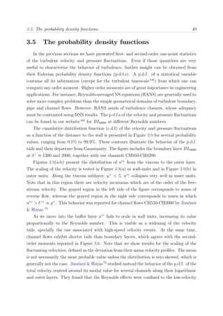
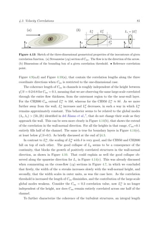
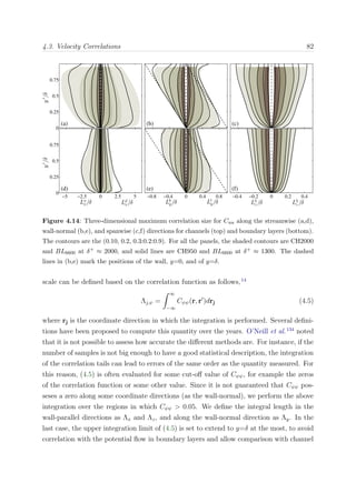
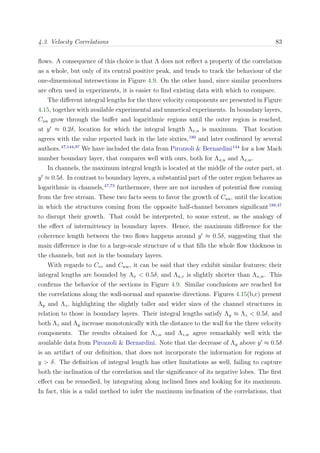
This document is the doctoral thesis of Juan A. Sillero Sepúlveda titled "High Reynolds Numbers Turbulent Boundary Layers". It contains acknowledgments, an index, and 6 chapters that study turbulent boundary layers at high Reynolds numbers through direct numerical simulation and analysis of one-point and two-point statistics, as well as velocity structures. The thesis was completed at the Polytechnic University of Madrid in June 2014 under the supervision of Dr. Javier Jiménez Sendín.


