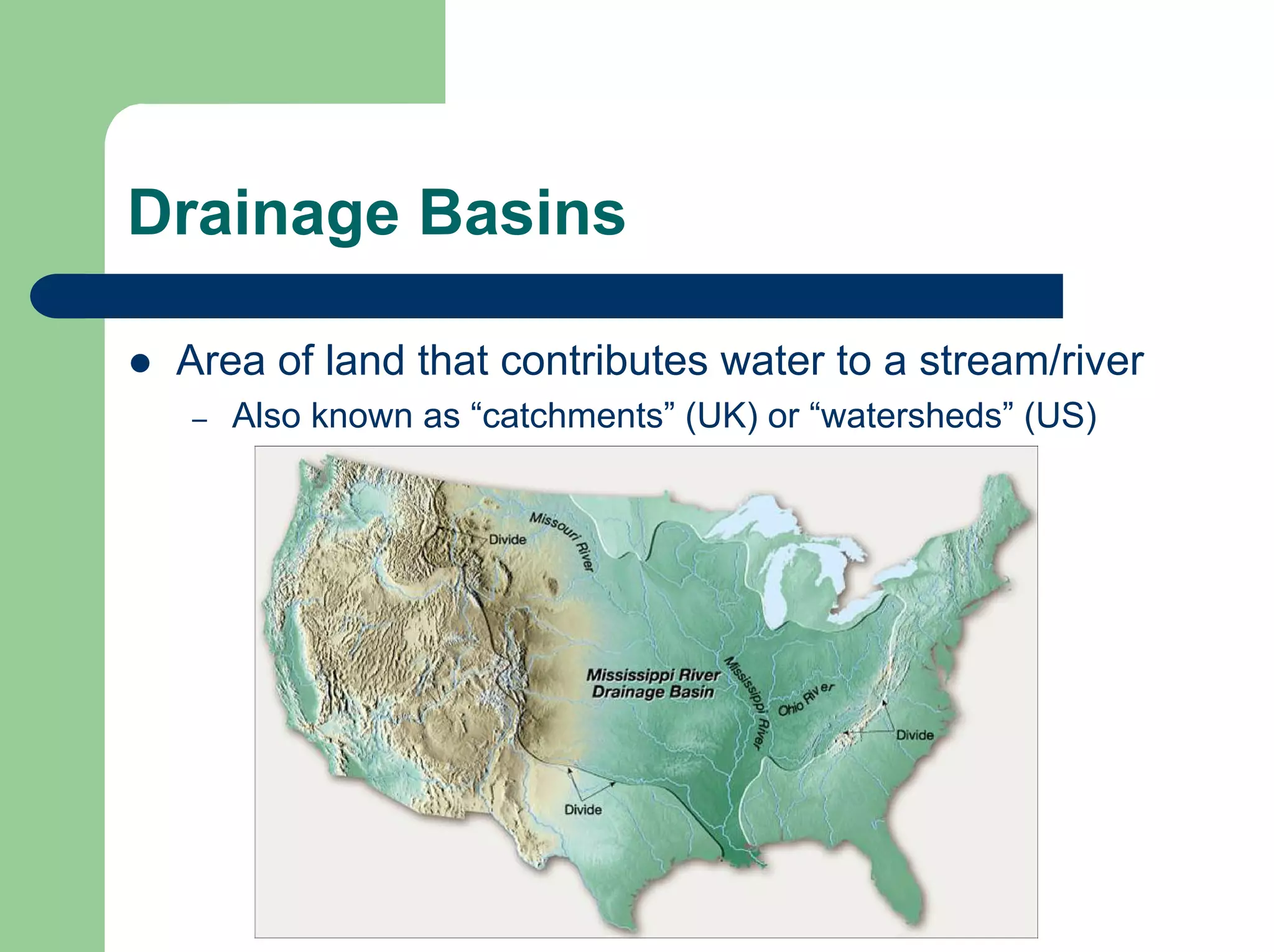
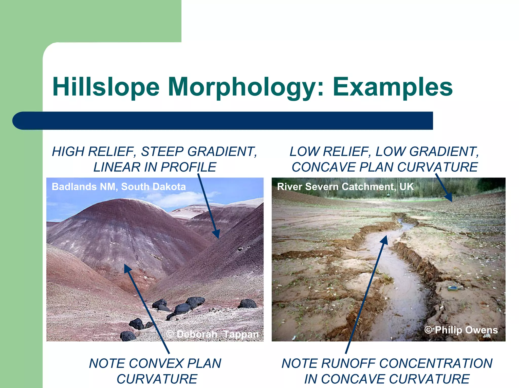
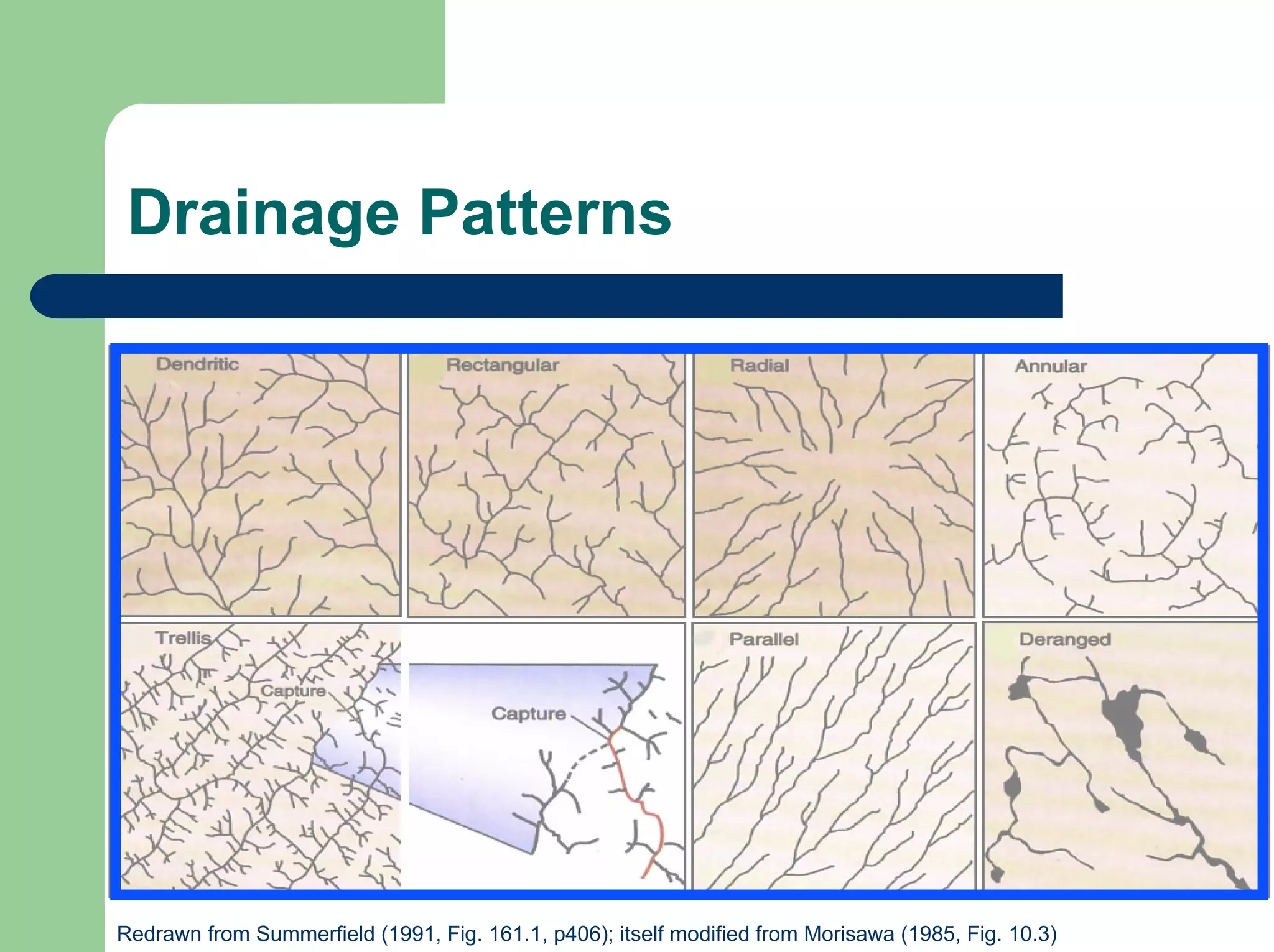
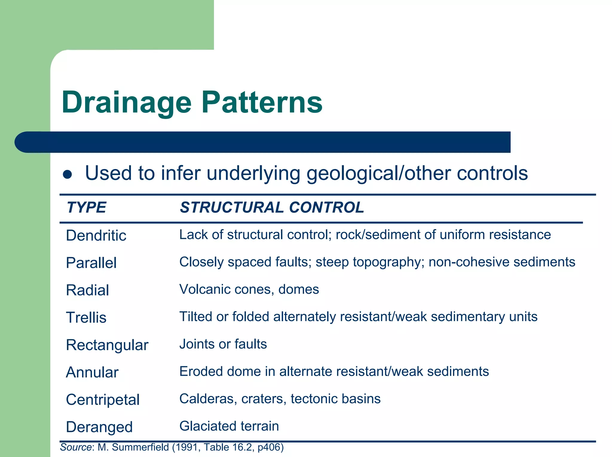
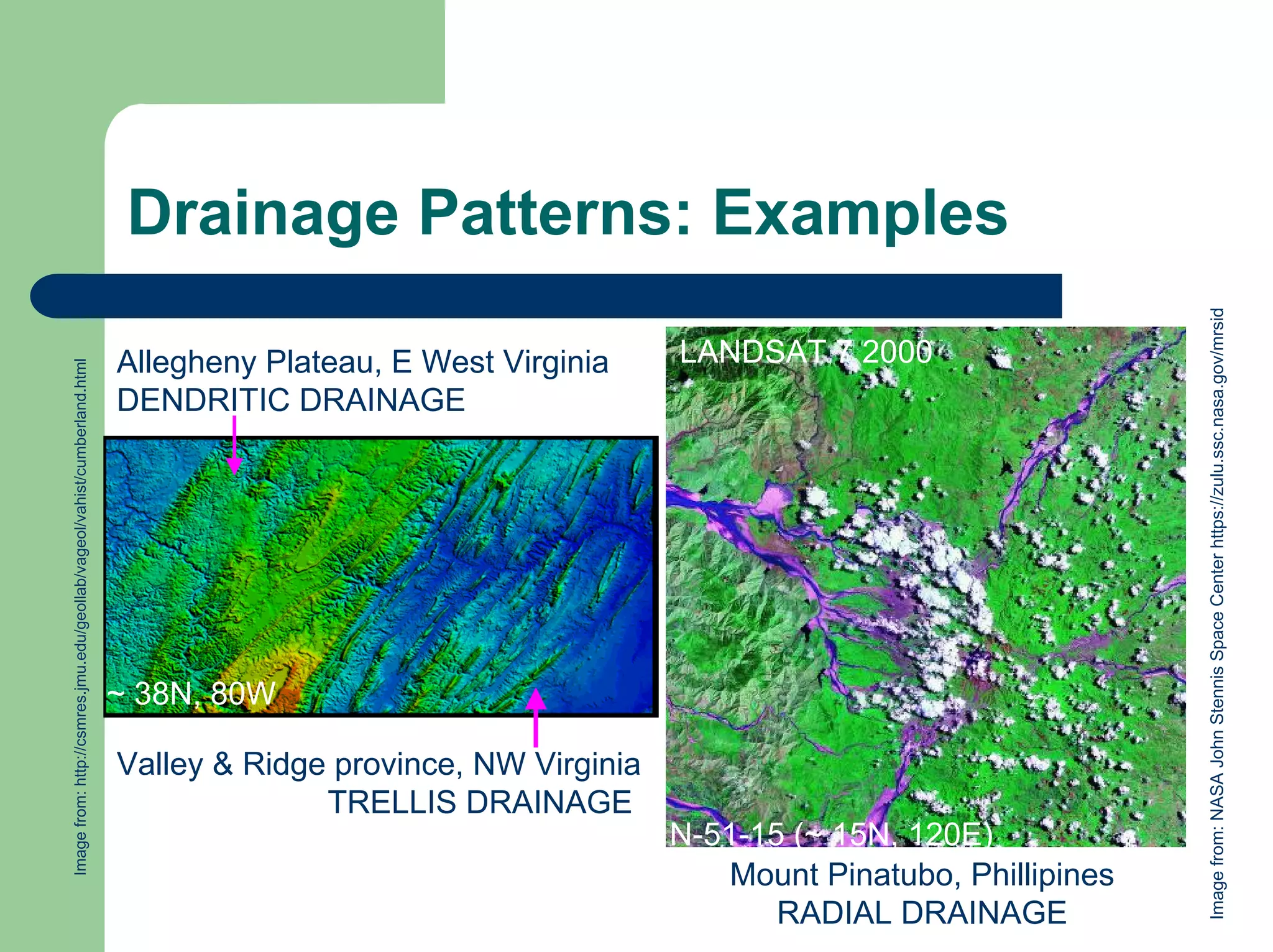
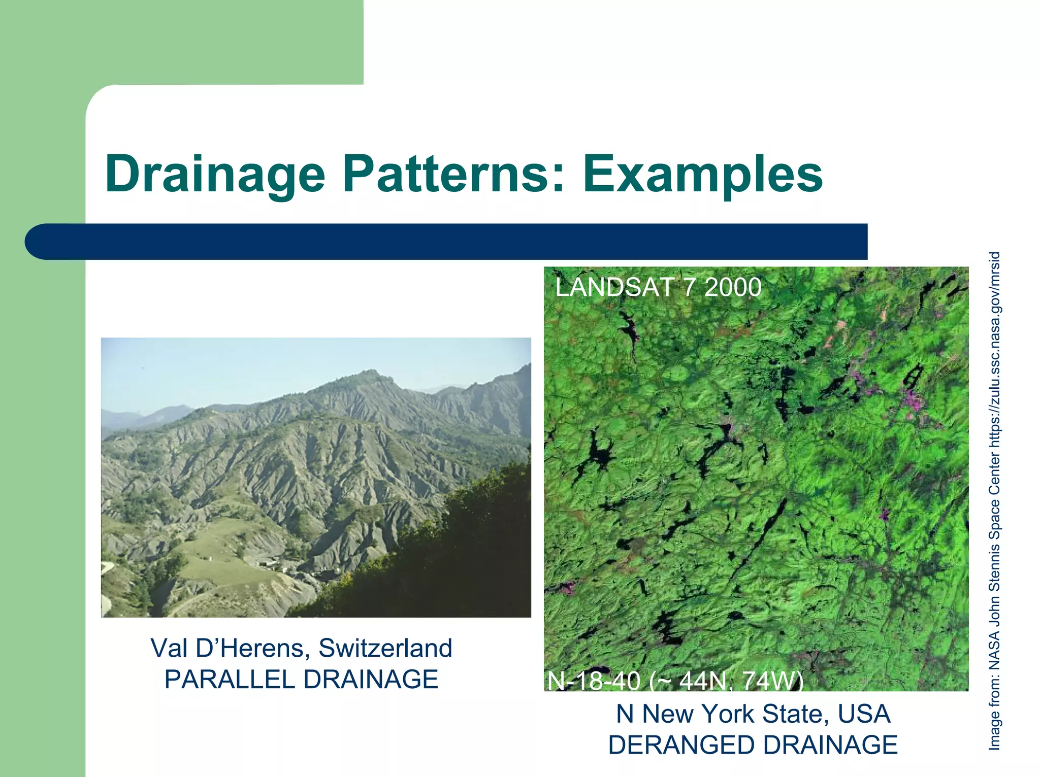
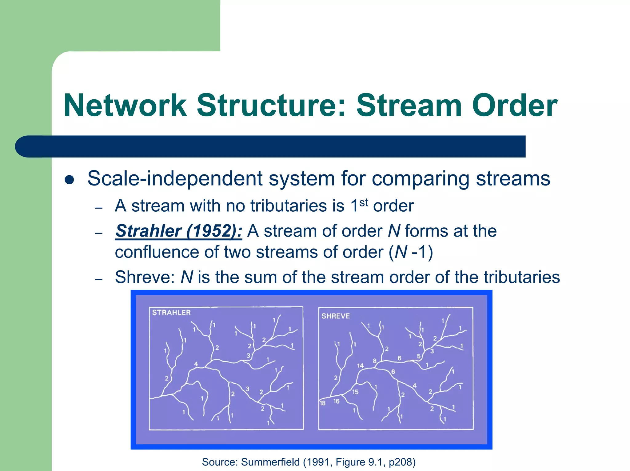
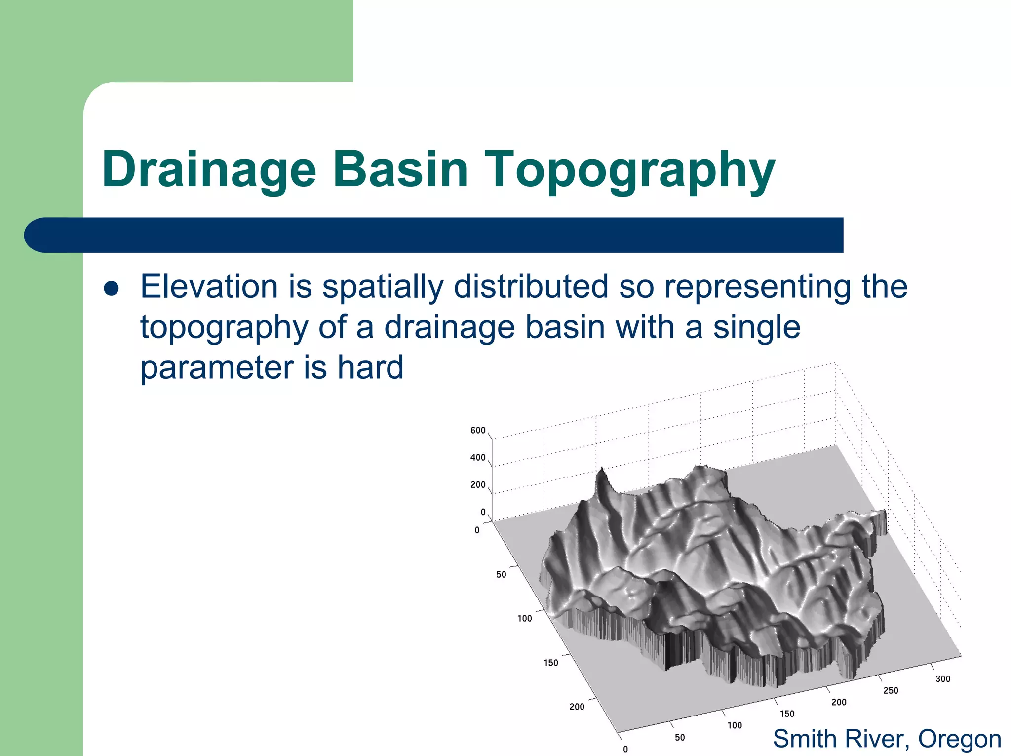
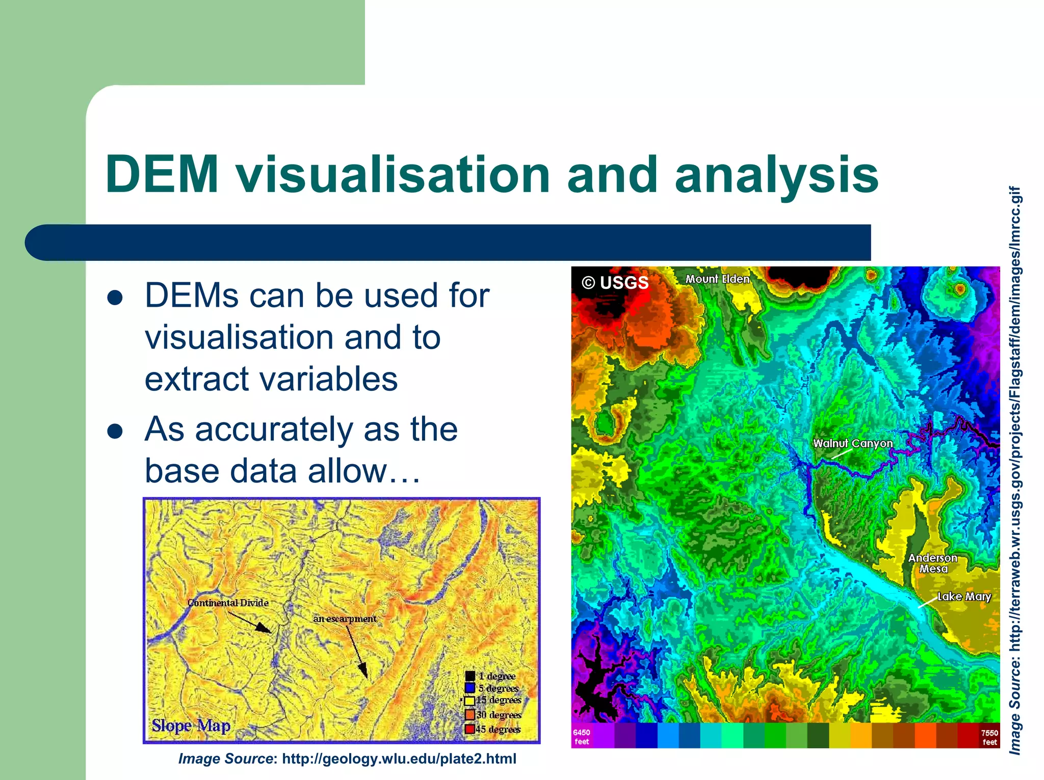
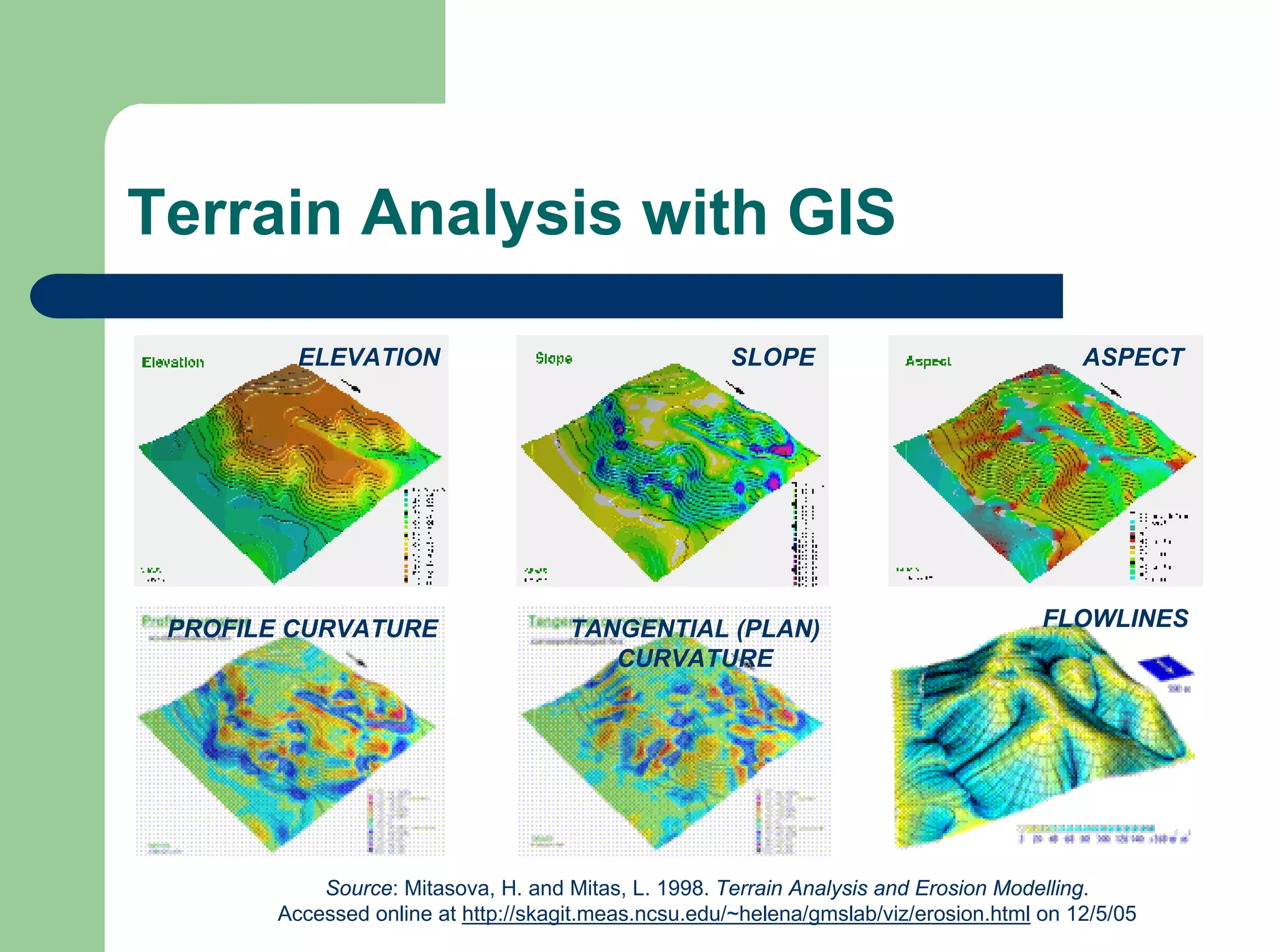
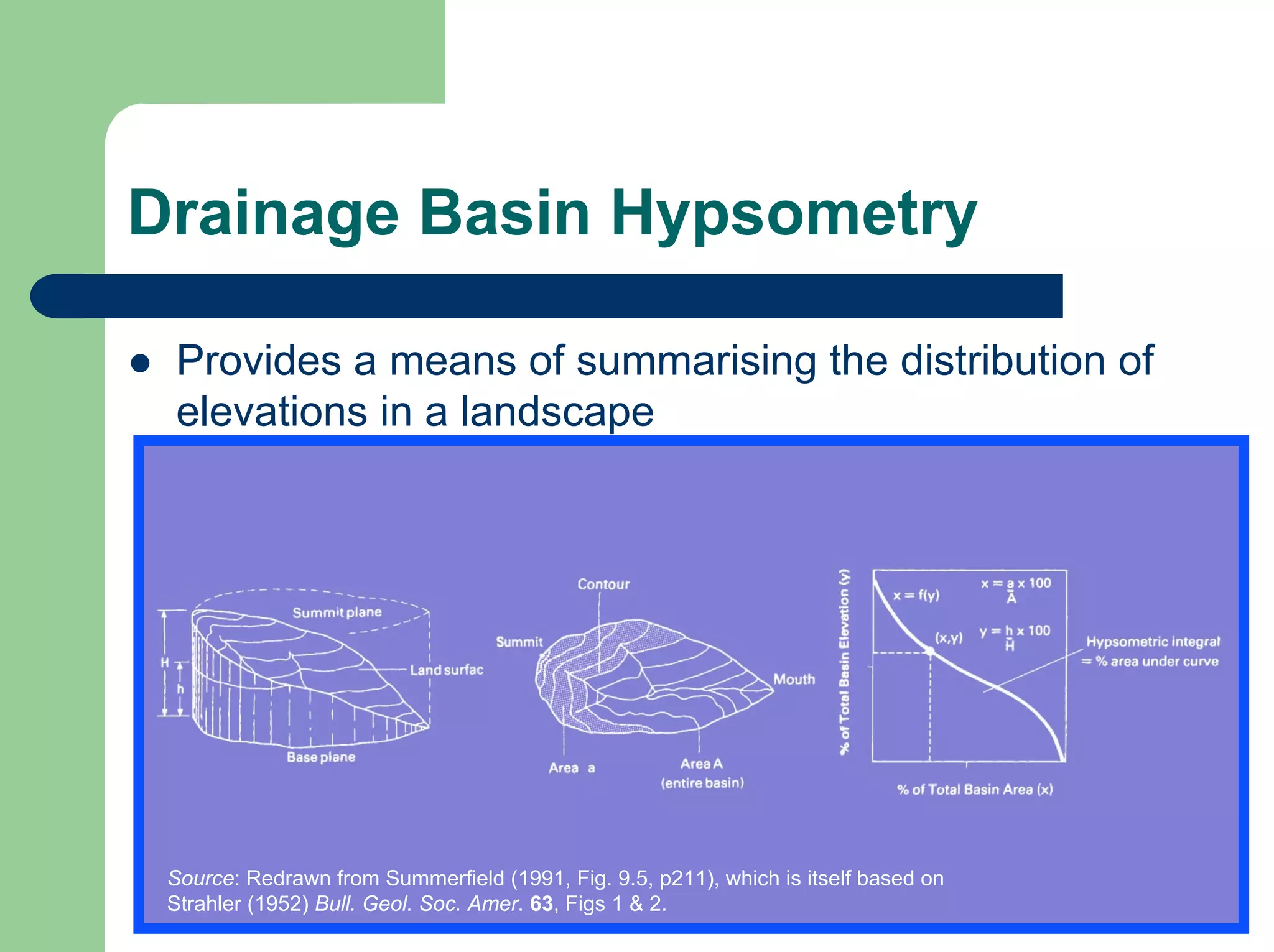
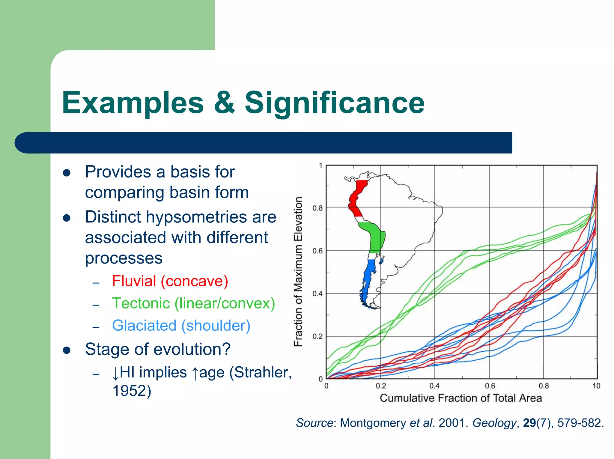
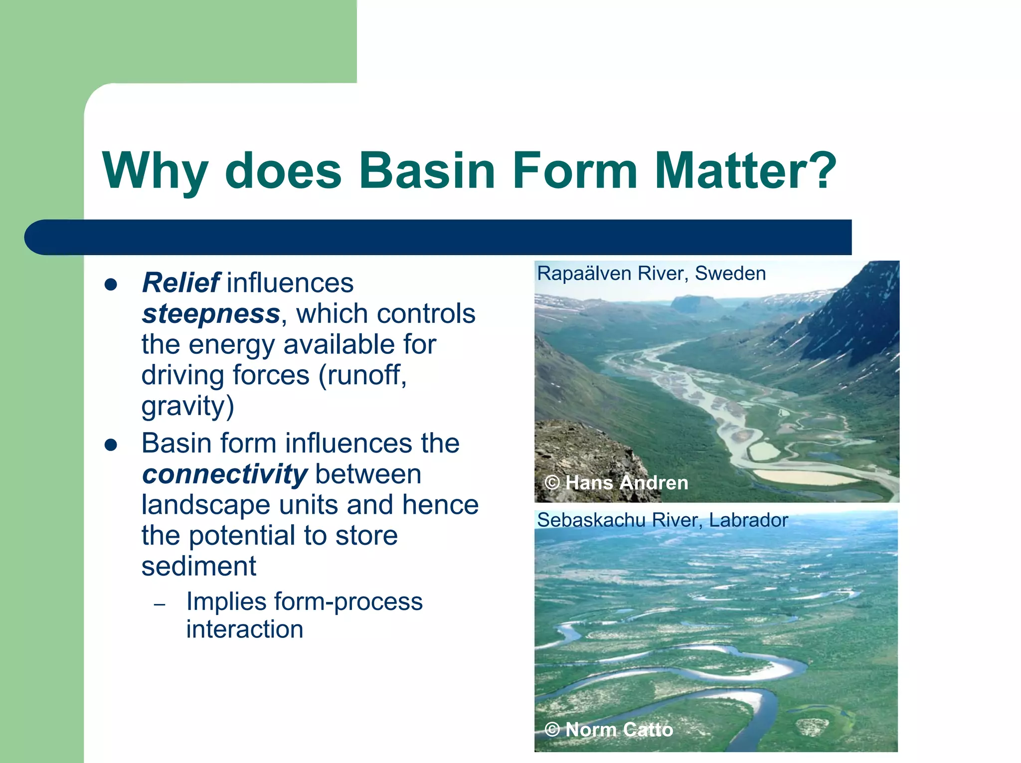
Drainage basin geomorphology can be summarized using morphometric analysis. Key variables include drainage patterns, stream order, basin shape, drainage density, relief, ruggedness, hypsometry, and topographic characteristics extracted from digital elevation models. Together these provide a quantitative description of basin form and allow comparison between basins. Basin form is influenced by climate, geology, and tectonics, and in turn influences hydrological and sediment transport processes within the basin. Morphometric analysis is needed to systematically describe basins and test hypotheses, but provides no direct insight into formative processes.

1. Drainage Basin Geomorphology
Fundamentals & Basin Morphometry
Source: http://www.ucmp.berkeley.edu/tectonics/globe1.gif
Dr Steve Darby

2. The Fluvial System: Components
z Sources, transfers, sinks
– (Schumm, 1977)
z Independent variables
– Climate, geology, land
cover/use, tectonics, etc
z Dependent variables
– See this lecture…
Source: Schumm, S.A. 1977. The Fluvial System, Wiley, New York

3. The Fluvial System: Functions
© Steve Darby
Mont Mine Glacier, Switzerland
z Terrestrial and aquatic
ecosystems
z Transports matter from
sources to sinks
– Water
– Solids (sediment,
organic matter, carbon)
– Solutes (mineral and
carbon solutes)
– Nutrients (N, P, etc)
LANDSAT
Image
from:
NASA
John
Stennis
Space
Center
https://zulu.ssc.nasa.gov/mrsid
S-45-05 (~8S, 143E)
LANDSAT 7 2000

4. Global Sediment Yield
z 70% of the total (15 000 Mt a-1) load comes from 10% of the land
– 3 rivers (Ganges, Brahmaputra & Huang He) carry 20% of the load
Source: Skinner, B. J., and Porter, S. C. (1995). The Dynamic Earth, An Introduction to Physical Geology (3rd Edition),
New York, John Wiley and Sons.

5. Global Denudation Rates
z Calculated by estimating total sediment/solute load
and dividing by basin area to give average ‘lowering
rate’ in mm ka-1
– Global mean is ~ 8 mm ka-1
z Masks huge variations amongst the world’s large
drainage basins
– Chari Basin, interior Africa (3 mm ka-1)
– Brahmaputra Basin, eastern Himalayas (677 mm ka-1)
z Scale dependent
– Haast River, Southern Alps, NZ (4,717 mm ka-1)
– Huangfuchan, China (19,814 mm ka-1)

7. The Scientific Method
Observation
Formulate ‘Theory’
(Hypothesis/Model)
Make Prediction
Test ‘Theory’ (Hypothesis/Model)
Robust Theory/Model/Hypothesis
Observation
New Observations
INDUCE
DEDUCE
PASS
REVISE
THEORY
?

8. Drainage Basins
z Area of land that contributes water to a stream/river
– Also known as “catchments” (UK) or “watersheds” (US)

9. Drainage Basin Components
z Boundaries
– Watersheds or divides
z Landscape elements
– Hillslopes
– Channels
– Channel heads
– Valleys
– Interfluves
z Materials
– Bedrock
– Regolith
– Colluvium vs. alluvium
HyMap airborne imaging spectrometer data (19 June 2000) draped over
DEM based on digitised OS 1:25 000 map contours for portion of Highland
Water Research Catchment, New Forest, UK

10. Drainage Basin Components
z Drainage divide/watershed
– Topographical
– Hydrological
– Military
z Interfluve
– A region of higher land
separating two rivers in the
same drainage basin
Source: Figure 14.4 from Christopherson, R.W. 2005.
Geosystems: An Introduction to Physical Geography
(5th
Edition), Prentice Hall, New Jersey.

11. Drainage Basin Components
z Hillslopes
– area of land between
drainage divide and a
channel or valley
z Channel
– a passage for water to flow
through
z Valley
– elongated lowland between
mountains, hills, or other
uplands, usually with a well
developed drainage
network
Photo courtesy of USGS photo library
Rocky Mountain NP, Colorado

12. Where do channels begin?
© Frans Kwaad 2002
Valley side gullies, Rif Mountains (N Morocco)

13. Channel Heads
Diffuse channel head
Rambla Mofar, near Turre, Almeria
© Professor Mike Kirkby
© Professor Mike Kirkby
Abrupt channel head
South of Lake Balaton, Hungary

14. Hillslope Morphology
z Hillslope morphology is complex and multi-dimensional, so
many parameters can be used as descriptors
– steepness, length, shape (i.e. rounded), degree of linearity,
concavity or convexity (in plan and/or in profile), etc.
z Hillslopes are usually mantled in sediment (colluvium)
– Sediment synonyms: Soil, regolith
z The significance of all these metrics is that water and gravity
mediated sediment transfer is strongly controlled by slope
– and the way in which slope varies across the landscape

15. Slope Profiles
Linear Hillslope Profile
0
2
4
6
8
10
12
14
16
18
20
0 20 40 60 80 100 120 140 160 180 200
Distance Across (m)
Elevation
(m)
z Basic hillslope profile shapes
– linear, convex, concave
– all have average slope of 0.1
Convex Hillslope Profile
0
2
4
6
8
10
12
14
16
18
20
0 10 20 30 40 50 60 70 80 90 100 110 120 130 140 150 160 170 180 190 200
Horizontal Distance (m)
Elevation
(m)
Concave Hillslope Profile
0
2
4
6
8
10
12
14
16
18
20
0 10 20 30 40 50 60 70 80 90 100 110 120 130 140 150 160 170 180 190 200
Distance Across (m)
Elevation
(m)

16. 3D Slope Morphology
Source:
http://www.soils.agri.umn.edu/academics/classes/soil5515/modules/topography/topography.html
z Hillslopes are 3-dimensional
z Slope curvature controls the
flow of surface and sub-
surface water across a
landscape
– areas with concave plan
curvatures have focused
flows, whereas convex
plan curvatures have
dispersed flows
– areas with convex profile
curvature have accelerated
flows, concave profile
curvature have
decelerating flows
L = linear, V = convex, C = concave

17. Hillslope Morphology: Examples
HIGH RELIEF, STEEP GRADIENT,
LINEAR IN PROFILE
NOTE CONVEX PLAN
CURVATURE
© Philip Owens
LOW RELIEF, LOW GRADIENT,
CONCAVE PLAN CURVATURE
River Severn Catchment, UK
NOTE RUNOFF CONCENTRATION
IN CONCAVE CURVATURE
© Deborah Tappan
Badlands NM, South Dakota

18. Drainage Basin Morphometry
z Morphometry
– The quantitative measurement of form
– Provides a systematic basis for description and comparison
(e.g. between basins, model predictions vs. observations)
z Topology versus topography
– Topological variables represent network structure
– Implies that two basins may look utterly different but be
functionally similar if their topology is similar
z Dimensional versus non-dimensional variables
– All things can be measured with 3 scales: M, L, T
– Dimensional: area (L2), velocity (L/T), density (M/L3)
– Non-dimensional: slope (L/L)
– Non-dimensional variables can be compared across basins
of different scale

19. Morphometric Variables
z Basic descriptions of basin shape & network structure
– Drainage patterns and network characteristics
– Basin size and shape (e.g. elongation ratio)
– Drainage density
z Topographic characteristics
– Analysis of slopes and curvature
– Basic mapping and DEM cartography
– Basin elevation
– Hypsometry
– Relief (local and total)
– Ruggedness

20. Drainage Patterns
Redrawn from Summerfield (1991, Fig. 161.1, p406); itself modified from Morisawa (1985, Fig. 10.3)

21. Drainage Patterns
z Used to infer underlying geological/other controls
TYPE STRUCTURAL CONTROL
Dendritic Lack of structural control; rock/sediment of uniform resistance
Parallel Closely spaced faults; steep topography; non-cohesive sediments
Radial Volcanic cones, domes
Trellis Tilted or folded alternately resistant/weak sedimentary units
Rectangular Joints or faults
Annular Eroded dome in alternate resistant/weak sediments
Centripetal Calderas, craters, tectonic basins
Deranged Glaciated terrain
Source: M. Summerfield (1991, Table 16.2, p406)

22. Drainage Patterns: Examples
Image
from:
NASA
John
Stennis
Space
Center
https://zulu.ssc.nasa.gov/mrsid
N-51-15 (~ 15N, 120E)
LANDSAT 7 2000
Mount Pinatubo, Phillipines
RADIAL DRAINAGE
Image
from:
http://csmres.jmu.edu/geollab/vageol/vahist/cumberland.html
Allegheny Plateau, E West Virginia
DENDRITIC DRAINAGE
Valley & Ridge province, NW Virginia
TRELLIS DRAINAGE
~ 38N, 80W

23. Drainage Patterns: Examples
Image
from:
NASA
John
Stennis
Space
Center
https://zulu.ssc.nasa.gov/mrsid
N-18-40 (~ 44N, 74W)
LANDSAT 7 2000
N New York State, USA
DERANGED DRAINAGE
Val D’Herens, Switzerland
PARALLEL DRAINAGE

24. Network Structure: Stream Order
z Scale-independent system for comparing streams
– A stream with no tributaries is 1st order
– Strahler (1952): A stream of order N forms at the
confluence of two streams of order (N -1)
– Shreve: N is the sum of the stream order of the tributaries
Source: Summerfield (1991, Figure 9.1, p208)

25. Some Data…
Wheeling Creek, Ohio
(2nd
Vs. 3rd
Order Basins)
Sulphur Creek, CA (2nd Order)
© Steve Darby
© Wheeling Jesuit University
z The largest river is the 12th order
Amazon
– Assuming 1st order streams are
identified correctly!
z Over 80% of the total length of
Earth’s rivers are 1st or 2nd order
z Basin area increases non-linearly
with increasing stream order
z Bifurcation Ratio (Rb)
– Rb = Nx/Nx+1
– Strahler says R is typically ~ 3
– Hence N1 > 175 000 for the
Amazon (N1 = 3x-1)
z Source areas make up in
numbers what they lack in size

26. Drainage Basin Shape
z Basin shape influences the fluxes and delivery of runoff and
sediment from headwater reaches
z Can be represented using the Elongation Ratio (E)
z E = (2/L)×(A/π)0.5
z E is dimensionless
Source: Redrawn from Benda, L. et al. 2004. Water
Resources Research, 40, W05402, doi:10.1029/2003WR002583.

27. Significance…
z Runoff delivery to streams
– Elongated basins have
flatter hydrographs
z Influences confluence
geomorphology (Benda et
al., 2004)
– Tributaries of elongated
basins have less impact on
main stem geomorphology
Source: Redrawn from Benda et al. 2004.

28. Drainage Density
z Extent to which a landscape is channelled reflects
the balance between erosive and resisting forces
– So, likely influenced by climatic and geologic factors
z Ratio of total stream length to drainage area (ΣSL/A)
z DD (has dimensions L-1) varies across a wide range
– e.g. 5 km-1 on permeable rocks, to 500 km-1 on badlands
z Can be problematic to define where channels are
indistinct or ephemeral
– Locating channel heads is critical to accurate estimation

29. Examples…
Images
from:
NASA
John
Stennis
Space
Center
https://zulu.ssc.nasa.gov/mrsid
N-14-40 (~ 40N, 100W)
LANDSAT 7 2000
N-19-05 (~ 5N, 70W)
LANDSAT 7 2000
LANDSAT 7 2000
N-19-05 (~ 5N, 70W)
LANDSAT 7 2000
Middle Loup River, Nebraska
SEMI-ARID - Low Drainage Density
Upper Orinoco Basin, Venezuela
HUMID - High Drainage Density

30. Physical Significance (?)
z Drainage density values can sometimes surprise
z Perhaps best interpreted as a long-term measure of
the relative difference between rainfall and infiltration
Nazca, Peru (~15S, 75W)
© Steve Darby

31. Drainage Basin Topography
z Elevation is the vertical height above a datum
z Relief (R) refers to differences in elevation at local (e.g. for a
hill) or total basin (difference in elevation between the drainage
divide and the basin outlet) scales
© Martin Geertsema
HIGH RELIEF
LOW RELIEF
HyMap
airborne
imaging
spectrometer
data
(19
June
2000)
draped
over
DEM
based
on
digitised
OS
1:25
000
map
contours
for
portion
of
Highland
Water
Research
Catchment,
New
Forest,
UK
~ 50m ~ 1000m

32. Drainage Basin Ruggedness
z Measured with the
ruggedness number
– RN = R × DD
z Measures the extent to
which basin topography
is dissected
DEM of the headwaters of the Smith
River in Oregon – an example of a rugged
basin with high relief

33. Drainage Basin Topography
z Elevation is spatially distributed so representing the
topography of a drainage basin with a single
parameter is hard
Smith River, Oregon

34. DEM visualisation and analysis
Image
Source:
http://terraweb.wr.usgs.gov/projects/Flagstaff/dem/images/lmrcc.gif
© USGS
z DEMs can be used for
visualisation and to
extract variables
z As accurately as the
base data allow…
Image Source: http://geology.wlu.edu/plate2.html

35. Terrain Analysis with GIS
Source: Mitasova, H. and Mitas, L. 1998. Terrain Analysis and Erosion Modelling.
Accessed online at http://skagit.meas.ncsu.edu/~helena/gmslab/viz/erosion.html on 12/5/05
ELEVATION SLOPE ASPECT
FLOWLINES
TANGENTIAL (PLAN)
CURVATURE
PROFILE CURVATURE

36. Drainage Basin Hypsometry
z Provides a means of summarising the distribution of
elevations in a landscape
Source: Redrawn from Summerfield (1991, Fig. 9.5, p211), which is itself based on
Strahler (1952) Bull. Geol. Soc. Amer. 63, Figs 1 & 2.

37. Examples & Significance
z Provides a basis for
comparing basin form
z Distinct hypsometries are
associated with different
processes
– Fluvial (concave)
– Tectonic (linear/convex)
– Glaciated (shoulder)
z Stage of evolution?
– ↓HI implies ↑age (Strahler,
1952)
Source: Montgomery et al. 2001. Geology, 29(7), 579-582.

38. Why does Basin Form Matter?
© Hans Andren
Rapaälven River, Sweden
Sebaskachu River, Labrador
© Norm Catto
z Relief influences
steepness, which controls
the energy available for
driving forces (runoff,
gravity)
z Basin form influences the
connectivity between
landscape units and hence
the potential to store
sediment
– Implies form-process
interaction

39. Conclusion
z Morphometric analysis is needed to provide a
systematic basis for describing & comparing
drainage basin geomorphology & to test hypotheses
z Morphometry can highlight links between basin
forms and environmental variables, but it provides no
direct insight into formative processes
z Care is required: Underlying data are derived from
maps, DEMs, etc.
– Relationships depend on the basic quality of acquired data
– Relationships can be scale dependent

40. Urumchi, NW China
© Matthias Jakob