Genetic programming (GP), created by Cramer in 1985 and later expanded by Koza in 1992, focuses on finding a function and its parameters to optimize a given function based solely on input-output data. The GP system operates differently from genetic algorithms, particularly in fitness evaluations, and utilizes programming languages like Lisp to handle chromosome structures, including operations such as crossover and mutation. Gene expression programming (GEP) is a newer approach that utilizes fixed-length chromosomes representing variable-length expressions, simplifying some of the complexities present in traditional GP methods.

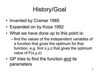
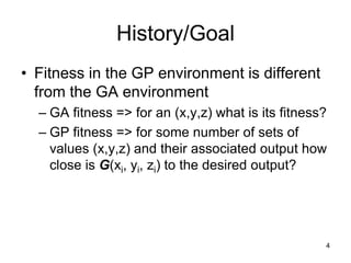
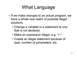
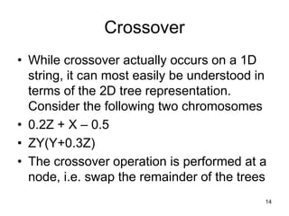
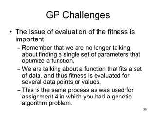
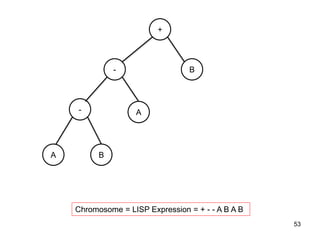
1. 1
Genetic Programming

2. 2
History/Goal
• Invented by Cramer 1985
• Expanded on by Koza 1992
• What we have done up to this point is:
– find the values of the independent variables of
a function that gives the optimum for that
function, e.g. find x,y,z that gives the optimum
value of F(x,y,z)
• GP tries to find the function and its
parameters

3. Goal
• What does it mean to find the function and
its parameters?
– We are trying to find the function for F(x,y,z)
such that given an (x,y,z), our function G
gives the same value as F(x,y,z). Generally
we don’t have F, all we have is inputs and
their outputs.
– This is a very different task from that
performed by a GA.
– In general this function G in GP is a program
3

4. 4
History/Goal
• Fitness in the GP environment is different
from the GA environment
– GA fitness => for an (x,y,z) what is its fitness?
– GP fitness => for some number of sets of
values (x,y,z) and their associated output how
close is G(xi, yi, zi) to the desired output?

5. 5
Attributes of a GP System (Goals)
• GP starts with what needs to be done – starts
from a high level description of the problem
• GP produces a result in the form of a program-
sequence of steps that can be run on a
computer – hence – real code
• GP can automatically determine the size of the
program, i.e. number of steps
• GP is largely problem independent
• Sometimes, GP produces results competitive
with humans

6. 6
What Language
• One of the challenges in developing a GP
environment is the issue of encoding, i.e.
in what form (language) should we encode
the solution.
– Remember, it is from this encoding that we
want to be able to do things like crossover
and mutate.
– As always, we don’t want illegal solutions
• In this case, what is an illegal solution?

7. 7
What Language
• A new challenge in GP is that we now
have a new realm of illegal solutions.
– Previously, an illegal solution was one in
which the changes to the parameters gave
them values that were in some way illegal,
e.g. X>100 or maybe we change X and Y so
that their sum exceeds some maximum even
though neither X or Y is larger than their
respective maximums. Or maybe we get a
divide by 0

8. 8
What Language
– If we make changes to an actual program, we
have a whole new realm of possible illegal
solutions.
• Change a variable in a statement to one
that is not declared
• Make an expression illegal, e.g. “+-”
• Create an illegal statement because of
type, number of parameters, etc.

9. 9
What Language
• The resolution of this issue requires a language
or an environment that embodies a structure that
can be manipulated, and has very “loose” rules
on parameter typing and declaration.
• LISP does this, and with certain restrictions we
can do it with other programming languages

10. 10
What Language
• LISP – List Processing, embodies these
characteristics
– An expression in LISP can be represented as
a linear (1D) string, which actually represents
a 2D expression.
– The expression 2*3+4 is represented in LISP
as (+ (* 2 3) 4) (called an S-expression). It
can also be represented as a tree.

11. 11
+
*
2 3
4
(+ (* 2 3) 4)

12. 12
LISP
• Consider the expression
• (+ 1 2 (IF (> TIME 10) 3 4))

13. 13
+
1
> 3
2
(+ 1 2 (IF (> TIME 10) 3 4))
IF
4
TIME 10

14. 14
Crossover
• While crossover actually occurs on a 1D
string, it can most easily be understood in
terms of the 2D tree representation.
Consider the following two chromosomes
• 0.2Z + X – 0.5
• ZY(Y+0.3Z)
• The crossover operation is performed at a
node, i.e. swap the remainder of the trees

15. 15
+
*
0.2 Z
X
-+(*0.2 Z) X 0.5
0.2Z + X – 0.5
-
0.5
*(* X Y)(+ Y (*Z
0.3)
ZY(Y+0.3Z)
*
*
Z Y
+
Y *
Z 0.3

16. 16
Crossover
• Let’s say that we perform the crossover at
the two (randomly selected) nodes labeled
with + for each of the two expressions
• In the next slide they are labeled in red
• Notice that although this is single point, it
is not the same point in each tree, and
thus the “chromosomes” can be of
different length. This is a very powerful
capability and can also be problematic

17. 17
+
*
0.2 Z
X
0.2Z + X – 0.5
-
0.5
ZY(Y+0.3Z)
*
*
Z Y
+
Y *
Z 0.3

18. 18
+
*
0.2 Z
X
(Y+(Z*0.3))-0.5
-
0.5
ZY(0.2Z + X)
*
*
Z Y
+
Y *
Z 0.3

19. 19
Crossover => Mutation
• Even in LISP there are some problems
with crossover, but the preceding at least
gives the idea of its implementation in a
GP environment using LISP
• The next question is how do we perform
mutation?

20. 20
Mutation
• Mutation can be most easily understood if
we first address the question of how do we
generate an initial program.
– We begin by deciding on a set of functions
(operators for now), and a set of terminals, i.e.
variables and constants. Generally the
variables with be the variables of the function,
e.g. F(x,y,z), x, y, and z are the variables
– We then randomly select from this set to
generate our program

21. 21
Program Generation
• As an example, let’s say we have the
following set:
– ,+, -, /, *, A,B,random_constant
• What are the lengths of the expressions
that can be generated?
• How many different programs can be
generated from this set?

22. 22
Program Generation
• Example set
– ,+, -, /, *, A,B,random_constant
• Let’s use 0=+, 1=-, … 8= random_constant
• Thus, generating a program simply means
generating a random sequence of integers
0 to 8. ( We will assume when we
generate an 8, we also generate a random
constant)

23. 23
Program Generation
• What would the string
– +,10.0,/,-,A,1.0,*,B,A
• This corresponds to the function
– 10.0 + (A-1.0)/(B*A)
• The tree would be

24. 24
Program Generation
+
10. /
- *
A 1 B A

25. 25
Program Generation
• What about the string + A B – A B?
• Note that it terminates after + A B, i.e. the
– - A B is not used
• Let’s say that we limit the length of a string
(program) to some maximum. Is there a
way to terminate it?

26. 26
Program Generation
• The problem we face is that when we get
to the maximum, we may not have a legal
or complete program or expression.
– Let’s say the maximum is 4 elements.
– + A – B is 4 elements long but not legal.
– How can we address this problem?

27. 27
Program Generation
• The problem we face is that when we get
to the maximum, we may not have a legal
program.
– Let’s say the maximum is 4 elements.
– + A – B is 4 elements long but not legal.
– How can we address this problem?
• When we get to the “max” length, we generate only
enough to make the string legal.
• What should this be?

28. 28
Program Generation
– Let’s say the maximum is 4 elements.
– + A – B is 4 elements long but not legal.
– How can we address this problem?
• When we get to the “max” length, we generate only
enough to make the string legal.
• What should this be?
– Just generate terminals (variables or constants)
until the string is legal

29. 29
Program Generation
• As an example:
– What will it take to make *,-,+,A,B,+,/,*,B
legal?
– It is easiest seen if we look at the tree.

30. 30
*
-
+ +
B
A /
*
B
* - + A B + / * B

31. 31
Program Generation
• As an example:
– What will it take to make *,-,+,A,B,+,/,*,B
legal?
– If we just randomly generate constants and
variables on the end we can “fill” out the tree.
– Let’ say we generate
– *,-,+,A,B,+,/,*,B,1.0,A,B,2.0
– We then get a completed tree:

32. 32
*
-
+ +
B
A /
*
B
* - + A B + / * B 1.0 A B 2.0
2.
B
A
1.

33. 33
Mutation
• Now that we have a way to randomly
generate a program(s), what happens on
mutation?
– Method 1
• Select a node at which to perform a mutation
• From that node down, remove all code
• Randomly generate another program segment
from that node down

34. 34
Mutation
– Method 2
• Only mutate operators for operators, and
terminals (variables and constants) for
terminals
– Method 3
• Select a node to mutate, and mutate it
• Let the interpreter be smart enough to
ignore extraneous code, or remove
extraneous code if need be.

35. 35
GP Challenges
• GP Problems/challenges
– Manipulation of the chromosome, while fairly
easy to visualize with a tree, requires more
challenging coding because of the linear LISP
string involved.
– The fact that the program is LISP means that
it will generally run slow, i.e. evaluation of the
fitness is an issue.
– The length of the chromosomes varies, and
over time some can/will grow very large if we
don’t limit its size
• To address length issue, we may have to
periodically “prune”, e.g. 5-4 becomes 1

36. 36
GP Challenges
• The issue of evaluation of the fitness is
important.
– Remember that we are no longer talking
about finding a single set of parameters that
optimize a function.
– We are talking about a function that fits a set
of data, and thus fitness is evaluated for
several data points or values.
– This is the same process as was used for
assignment 4 in which you had a genetic
algorithm problem.

37. Fitting Data - Parsimony
• The rule to generally go by is that when
given the choice between two functions
used to fit a set of data, choose the
simpler of the two functions. This is
minimizing parsimony
– Why?
• It is a fact that for any set of N data points, a (N-1)
or higher degree polynomial will fit the data
perfectly.
• The problem lies in the details, i.e. even though the
function fits the data perfectly, what happens
between the data points?
37

38. 38
GP Challenges
• Thus, as the GP grows, there is a
tendency to expand in terms of program
length and program complexity.
• Some of this problem can be reduced by
“pruning” the trees after every few
generations, but that slows the whole
process.

39. 39
Tree Pruning
• The process of pruning the tree of a Lisp
program, involves replacing degenerate
cases, e.g.
– (= 1 1) could be replaced with true
– (+ 1 1) could be replaced with 2
• There are obviously other issues with this
process since it changes the tree which
may impact what happens under
crossover and/or mutation. But in general,
pruning is good.

40. Pros and Cons of GP
• While LISP is still used in some GP
environments, there has been
considerable work in developing GP
environments which use other languages.
• With variable length chromosomes, there
is also the challenge of controlling the
length of programs as they evolve.
40

41. 41
GEP – A Modified Approach to
Genetic Programming
• Gene Expression Programming (GEP) is a
relatively new technique developed by
Candida Ferreira - ~2000
• In this case, the chromosomes are of fixed
length, whereas the expression lengths
vary within some limit.
• Like GP, each chromosome represents a
program (for now it will just be an
expression)

42. 42
GEP Material
• In addition to these notes, there are several
papers on GEP on the WEB.
• Some are located at:
• http://www.gene-expression-
programming.com/webpapers/GEPtutorial.pdf
• http://gene-expression-
programming.com/webpapers/GEPfirst.pdf
• The GEP web site also includes extensive
tutorials

43. 43
GEP
• What makes GEP somewhat unique is
that its fixed length chromosome can
represent variable length expressions.
• A GEP chromosome consists of two parts,
a head and a tail. The head is any
combination of operators and operands
(terminals and non-terminals). The tail is
any combination of operands (terminals)
• Remember this distinction!
• A constant is considered an operand

44. GEP
• The head of a GEP expression is a
random string of operators and operands.
• The tail of a GEP expression is a random
string of operands
– Remember what we had to do to the LISP
expression to “fill it out?”
• We added operands
• The tail length is chosen so that no matter what is
in the head, there are enough terminals in the tail
to complete the expression.
44

45. GEP
• GEP strings look like the LISP strings we
have seen, except:
– The length of the head is fixed
• And thus, the length of the tail can be
derived from the length of the head and the
arity (number of operands) of the operators.
–While the strings look alike, the building
of the equivalent tree and its evaluation
is slightly different
45

46. 46
GEP Length
• The length of the head is set by the user.
Call it H
• The length of the tail is determined from
the length of the head – H
• The length of the tail T is a function of the
length of the head H, and the maximum
arity of any of the operators n

47. 47
GEP Length
• The arity of an operator is the number of
operands that operator requires.
– Arity of square root is 1
– Arity of * is 2
– Arity of – is 1 (unary minus) or 2 (subtraction)
– GEP even allows for arity > 2, e.g. ternary
addition
• The total length of a GEP chromosome is
Head length (H) + Tail length (T), i.e.
T= H*(n-1)+1

48. 48
GEP Length
• Thus for a head of length 10, and unary
and binary operators, the tail would be of
length
– T=10*(2-1) +1 = 11
– Total Chromosome length = 10 + 11 = 21
• For a head of length 10 and unary, binary
and ternary operators
– T=10*(3-1) + 1 = 21
– Total Chromosome length = 10+21 = 31

49. 49
GEP Length
• Let’s say that we have a head length of 3,
only the + & - operators, and two variables
or operands A and B. What will be H, T,
and the total length?
– Since it is the + operator, the maximum arity
is 2.
– H is given as 3
– Thus
• T=H*(n-1)+1 = 3*(2-1)+1 = 4
– How will this maximum arise?

50. 50
GEP Length
• How will this maximum arise?
• Consider the case of the head consisting
of only the operators, i.e. + - -, what must
be the tail?
– The tail must be 4 operands – A’s and B’s
– The next slide shows the tree for such an
arrangement

51. 51
-
+
-
A B A B
Chromosome = GEP Expression = + - - A B A B

52. NOTE
• Note that in this case the GEP tree is built
differently from the LISP tree.
• If the expression +--ABAB had been for a
LISP expression, then the tree would be:
52

53. 53
-
+
-
B
A
A B
Chromosome = LISP Expression = + - - A B A B

54. 54
GEP Example
• Consider the following expression
• The tree for this expression would be:
e
-
d
*

c
b
a

55. 55
• The GEP string for the preceding would be:
• The integers above the string are simply to index
the elements

56. GEP Trees
• If you have been watching, you have
noticed that a GEP tree for a chromosome
is not the same as the expression tree that
we built for a LISP expression.
– The reason is that the tail of the GEP
expression may have only terminals. Thus for
a maximum length GEP chromosome (one
with no unused elements), the tail must be for
the last row or level of the tree – all terminals.
56

57. 57
Question
• What tree would the following K-
expression (that’s what Ferreira calls
them) code for? (Q is square root)

58. 58

59. 59
More GEP’s
• Consider a chromosome for which the set
of functions is F = {Q, *, /, -, +} and the set
of terminals is T = {a, b}.
• In this case, n = 2 (max arity); and if we
chose an h = 15, then t = 16.
• The length of the gene g is 15+16=31.
• One such gene is
0123456789012345678901234567890
/aQ/b*ab/Qa*b*-ababaababbabbbba

60. 60
GEP’s
• Now draw the tree for this expression

61. 61

62. 62
What happens if?
• What happens if at position 2, the Q
(square root) is changed to a “+”?
0123456789012345678901234567890
/a+/b*ab/Qa*b*-ababaababbabbbba
What is the new tree?

63. 63

64. GEP IDE
• The GEP IDE is a very large and well
documented GP environment.
• It does not have the functionality to
generate all categories of programs;
however, if the “function” can be
represented as an expression, then GEP
has the potential to find the “best”
expression.
64

65. GEP Environment
• Like Matlab, GEP has the ability to read in
Excel files for the data.
• Once a GEP expression has been derived,
GEP can generate an equivalent program
in a multitude of different languages.
• GEP reads as its input from an Excel file
65

66. GEP IDE
66

67. Important Note On GEP
• When inputting an Excel file of data as
training or test REMEMBER:
– Insert a row of dummy values as the first row;
otherwise it only reads N-1 rows
– Be sure to see that the last column is the one
used for the predictable or target. Because
GEP labels the columns like A1, A2,.. It then
orders them alphabetically. What this means
is A9 comes after A45. If A45 is the last or
predictable value, you need to set it as such
67

68. Example
• For this example, we will use the H4 Data.
Instead of finding the parameters as in
homework 4, we will find the function and
parameters for the data.
• Note that the function derived will likely be
very different from the one we used to
generate the data.
68

69. A B C D E F OUT
3.651405 -2.60247 7.378754 4.4934 8.283131 77.82019 34.26497
1.831271 -0.11943 5.57562 -3.57578 7.951177 26.17905 -3.95293
2.550929 -4.66467 21.56286 -1.27206 2.020111 35.72745 10.93247
2.304536 -4.54927 20.18452 -3.21892 0.396615 96.96078 8.475999
2.508332 -4.11504 6.332095 1.86956 0.225546 84.38288 27.59149
4.379797 -0.25062 1.321408 2.735182 3.972376 38.5376 29.15822
4.700903 -0.38833 18.1707 -2.80373 0.215971 33.13248 9.315848
3.347355 -3.64873 16.60594 0.804735 1.539553 49.19623 21.27661
1.973178 1.636113 20.82038 1.369196 8.287639 6.336365 10.2556
1.052932 0.549494 18.28929 -0.41666 1.463885 58.2357 13.37768
69

70. Example
• The next few slides are screen shots of opening
GeneXpro (The IDE name for the GEP system)
and loading the data, etc.
• Screen A
– Select New to create a new GEP solution
• Screen B
– This is H4Example, function finding and the data will
come from an excel file, select Next
• Screen C , D, and E
– Inputting the data
– Click on the green “+” to get screen D
– Click on “…’ to browse for the file, then click “OK” to
load it – The file must be .xls

71. Example
• Screen C , D, and E Input the data
– Click on the green “+” to get screen D
– Click on “…’ to browse for the file, then click
“OK” to load it – The file must be .xls
– If all is loaded correctly, you will see screen E
• You really only need to be concerned about the
lower part of the window where the columns of the
spreadsheet are given. The predictable column is
the desired or target output. If you have the wrong
column for predictable, then click on that element
and change its type to predictable.
– If all is correct, click on Load to load the file

72. 72

73. 73

74. 74

75. 75

76. 76

77. Important Note On GEP
• When you select data source for training –
– test the connection to see that it is valid.
– The two windows will be filled in. The bottom
window will show the data items with names
like A1, A2, …
• Remember, the last one which is called
(predictable) is the alphabetically last one. You will
have to move through to find the real last one, then
select it, select type->predictable, and that will do
it.
77

78. GEP IDE Example
• If the data has loaded properly, you will
seen the screen on the next overhead
– Note that the left scrollable window shows the
data. At the bottom of the window is a
summary of the number of rows and columns
read in.
– If you click on next, you will have the
opportunity to read in testing data. For this
example, we will not do so. We will simply
select finish.
78

79. 79

80. GEP IDE Example
• Once finished, you will be given the option
to save your GEP environment. It is wise
to do so.
• After saving your environment, you will
have the opportunity to configure GEP and
run it. The next slide shows the home
window.
80

81. 81

82. GEP Example – “The Hard Part”
• Although one could simply select evolve to
run GEP, the results would not be very
informative without understanding how to
set up for a run.
• Remember that there is a Matlab-like help
function in GEP
– Select Help=> GeneXpro Tools Help
• In the following slides, we will briefly
review
82

83. GEP Example – “The Hard Part”
• In the following slides, we will briefly
review the following tabs
– Evolve/optimize/simplify/stop
– Data
– Settings
– Functions
– Run
– Results
– Model
83

84. GEP - Evolve/optimize/simplify/stop
• If you select Evolve, the system will create
a random population of GEP
chromosomes and begin to evolve.
• Selecting Stop will cause the evolution to
stop (See next slide)
84

85. 85

86. GEP - Evolve/optimize/simplify/stop
• The plots on the preceding slide should be
self-explanatory
• Note that in addition to the Evolve button
being active, the optimize and simplify
buttons are active. Selecting optimize will
cause the system to continue to evolve
using the population it had when it
stopped. Selecting evolve will cause the
system to generate a new initial
population, i.e. it will start over.
86

87. GEP - Evolve/optimize/simplify/stop
• Selecting simplify will cause the system to
continue to evolve but with parsimony
pressure added to give greater weight in
selecting mates to those models that are
simplest.
87

88. GEP - Data
• The Data tab allows you to view your
training data, change it, and/or add testing
data
88

89. 89

90. GEP - Settings
• The Settings option is what you use to
actually define your GEP environment.
• There are 4 setting tabs
– General Settings
– Fitness Function
– Genetic Operators
– Numerical Constants
90

91. General Settings
• Training Samples – Given, it’s the number
of data elements to train on
• Testing Samples – Disabled unless there
is a testing file
• Number of chromosomes- This is the size
of your population – experiment
• Head Size – Depending on the max atiry
of your operator set, this will determine the
chromosome length
91

92. General Settings
• Number of Genes- Each chromosome is
made of 1 to n genes. The size specified
by head size is actually the size of each
gene.
• Linking function – This is how the values
of the genes are linked to give a single
value for the chromosome, e.g. addition
means they are added together.
92

93. General Settings
• Complexity Increase (If enabled)
– Generations without change: After X
generations without an improvement in the
best fitness, a gene is added.
– Number of tries: This is the number of times a
gene will be added
– Max Complexity: Maximum number of genes
allowed
93

94. 94

95. Fitness Function
• Fitness function – Too many to detail. Use
help to define them. In our example we will
use the standard RMSE (root mean
squared error)
• With Parsimony pressure – fitness is
reduced as the gene gets more complex
• Selection range – if the error is > selection
range, it is ignored in computing the
overall error
95

96. Fitness Function
• Precision – for hits, if the output is within
precision of the target the error is 0.
• 0/1 Rounding threshold – For 0/1 outputs,
values above the rounding threshold
become 1, else 0.
96

97. 97

98. Genetic Operators
• Mutation default 0.044
– Rule of thumb is an average of 2
mutations/chromosome
– No constraints on the kinds of mutations,
except to maintain structurally correct
programs
– Best of each generation is cloned, i.e. not
changed
98

99. Genetic Operators
• Inversion 0.1
– Only occurs in heads
– Given a chromosome, if random #< Inversion,
then
• Randomly choose gene to invert
• Randomly choose position in gene and length to
invert
• Invert, e.g. +ab => ba+
99

100. Genetic Operators
• IS transposition: 0.1
– Insertion Sequence
– A short fragment of a gene, position and
length randomly chosen
– This fragment is then inserted into the head
(not the root node) of another randomly
chosen gene, and elements deleted at the
end of the head of that gene to accommodate
the inserted fragment
100

101. Genetic Operators
• RIS Transposition: 0.1
– Root insertion sequence
– Element must start with a function (operator)
– Starts at a random location in the head and
scans until it finds a function. Then moves
down the head a random number of elements,
copies that string and inserts it at the front
(root) of the head.
– Extras at the end of the head are deleted to
make room
101

102. Genetic Operators
• One-point recombination: 0.3
– Same as single point recombination
– Recombination rate is probability of genes
combining
• Two-point recombination: 0.3
– Same as one-point except start and end
points are chosen
102

103. Genetic Operators
• Gene Recombination: 0.1
– Like one-point recombination except
individual genes are swapped
• Gene Transposition: 0.1
– Randomly select a gene and move it to the
from and delete the old gene
– Generally of little impact except for linking
functions of subtract and divide
103

104. 104

105. Numerical Constants
• For numerical constants, GEP generates a
string of random values for each gene of
length equal to the length of the tail. Each
random number has a position 1-T. In
generating a gene, if a random number is
chosen, then only its position in the string
of random values in encoded into the
gene.
105

106. Numerical Constants
• Select – Use Random numerical constants
– Will generate 0 to N random numerical
constants/gene within the given lower/upper
bounds. Type will be integer or floating-point.
• RNC mutation: 0.1
– Mutates the string of random numerical
constants
• DC Mutation:0.044
– Mutates the index or pointer of a numerical
constant, i.e. which one of the numerical
constants is used 106

107. Numerical Constants
• DC Inversion & transposition
– These two operators work like their
counterparts except the operation is carried
out on the string of random numerical
constants.
107

108. 108

109. GEP - Functions
• The functions operators allows the user to
select which functions (operators) to be
used.
109

110. GEP – Run, Results, Model
• Run
– Allows one to evolve, simplify, etc.
• Results
– Display the results of the evolution
• Model
– Save the model in code of choice
110

111. MS Thesis Topics
• A
– Use Weka to build a decision tree
– Convert the tree into a GEP like expression
– Generate a population of such trees and then
use GEP to evolve
• B
– Use GEP directly to evolve a decision tree
– Note: a GEP expression is a tree. If we use
If/then/else as only operator, is it a decision
tree? 111

112. GEP for Classification
• When using GEP for classification there
are a few differences:
– Chose “Classification” as the run category
– Read the data in as before but remember
there can only be two output values 0 or 1
– Most things can remain the same except
• The fitness function choices change (see help)
• You must pick a 0/1 rounding threshold
• For the homework, number of hits will work
– The output is different 112

113. 113