Downloaded 38 times


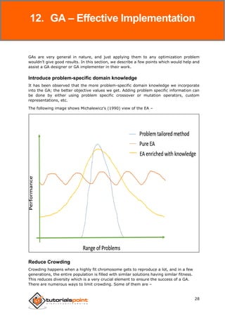
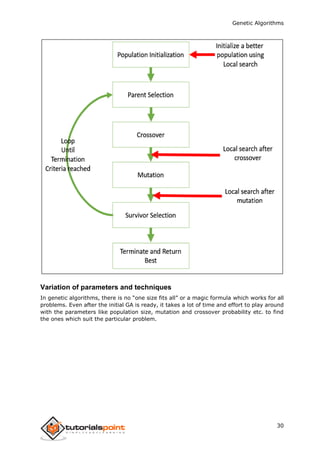

This tutorial covers the key concepts of genetic algorithms (GAs), a search-based optimization technique that employs principles of genetics and natural selection to find optimal solutions efficiently. It is intended for students and researchers familiar with programming and basic algorithms, and discusses various components such as population initialization, fitness functions, and genetic operators like crossover and mutation. The document also addresses the advantages and limitations of GAs, positioning them as effective tools for solving complex optimization problems that traditional methods struggle with.


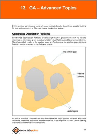
![[Deck] What's New in Spark-Iceberg Integration via DSV2.pptx](https://cdn.slidesharecdn.com/ss_thumbnails/deckwhatsnewinspark-icebergintegrationviadsv2-260210005337-25955b12-thumbnail.jpg?width=640&height=640&fit=bounds)


