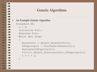
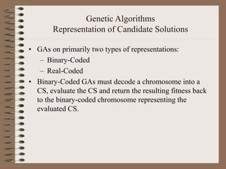
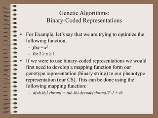
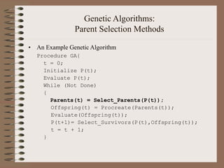
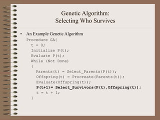
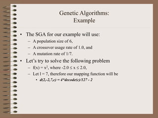
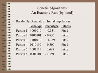
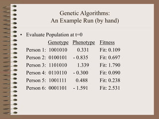
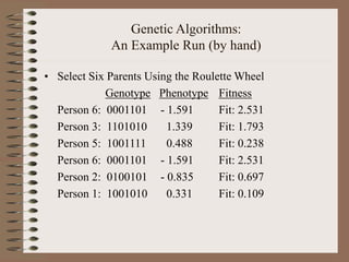
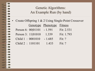
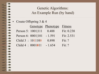
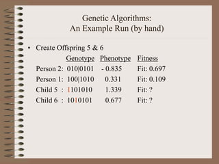
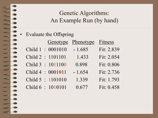
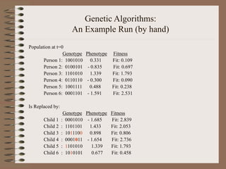
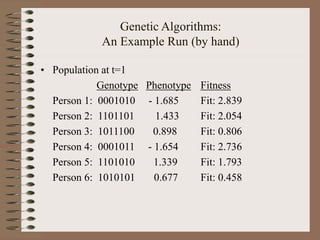
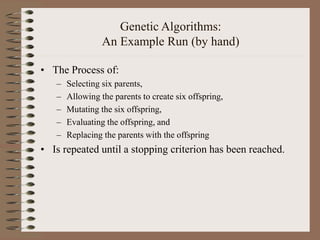
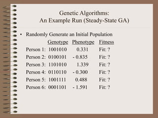
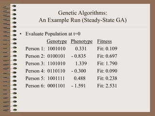
The document describes genetic algorithms and their components. It provides an overview of a basic genetic algorithm procedure that initializes a population, evaluates it, selects parents, generates offspring through crossover and mutation, evaluates the offspring, and selects survivors for the next generation. It then discusses various representations, selection methods, crossover and mutation operators, and replacement strategies for genetic algorithms. Finally, it walks through a simple example of applying a genetic algorithm by hand to optimize a function.

1. Genetic Algorithms
• An Example Genetic Algorithm
Procedure GA{
t = 0;
Initialize P(t);
Evaluate P(t);
While (Not Done)
{
Parents(t) = Select_Parents(P(t));
Offspring(t) = Procreate(Parents(t));
Evaluate(Offspring(t));
P(t+1)= Select_Survivors(P(t),Offspring(t));
t = t + 1;
}

2. Genetic Algorithms
Representation of Candidate Solutions
• GAs on primarily two types of representations:
– Binary-Coded
– Real-Coded
• Binary-Coded GAs must decode a chromosome into a
CS, evaluate the CS and return the resulting fitness back
to the binary-coded chromosome representing the
evaluated CS.

3. Genetic Algorithms:
Binary-Coded Representations
• For Example, let’s say that we are trying to optimize the
following function,
– f(x) = x2
– for 2  x  1
• If we were to use binary-coded representations we would
first need to develop a mapping function form our
genotype representation (binary string) to our phenotype
representation (our CS). This can be done using the
following mapping function:
– d(ub,lb,l,chrom) = (ub-lb) decode(chrom)/2l-1 + lb

4. Genetic Algorithms:
Binary-Coded Representations
• d(ub,lb,l,c) = (ub-lb) decode(c)/2l-1 + lb , where
– ub = 2,
– lb = 1,
– l = the length of the chromosome in bits
– c = the chromosome
• The parameter, l, determines the accuracy (and resolution
of our search).
• What happens when l is increased (or decreased)?

5. Genetic Algorithms:
Binary Coded Representations
Individual
Chromosome: 00101
Fitness = ?????
d(2,1,5,00101) = 1.16 f(1.16) = 1.35
Individual
Chromosome: 00101
Fitness = 1.35
The Fitness Assignment Process for Binary Coded
Chromosomes (ub=2, lb=1, l=5)

6. Genetic Algorithms:
Real-Coded Representations
• Real-Coded GAs can be regarded as GAs that operate on
the actual CS (phenotype).
• For Real-Coded GAs, no genotype-to-phenotype mapping
is needed.

7. Genetic Algorithms:
Real-Coded Representations
Individual
Chromosome: 1.16
Fitness = ?????
f(1.16) = 1.35
Individual
Chromosome: 1.16
Fitness = 1.35
The Fitness Assignment Process for Real Coded Chromosomes

8. Genetic Algorithms:
Parent Selection Methods
• An Example Genetic Algorithm
Procedure GA{
t = 0;
Initialize P(t);
Evaluate P(t);
While (Not Done)
{
Parents(t) = Select_Parents(P(t));
Offspring(t) = Procreate(Parents(t));
Evaluate(Offspring(t));
P(t+1)= Select_Survivors(P(t),Offspring(t));
t = t + 1;
}

9. Genetic Algorithms:
Parent Selection Methods
• GA researchers have used a number of parent selection
methods. Some of the more popular methods are:
– Proportionate Selection
– Linear Rank Selection
– Tournament Selection

10. Genetic Algorithms:
Proportionate Selection
• In Proportionate Selection, individuals are assigned a
probability of being selected based on their fitness:
– pi = fi / fj
– Where pi is the probability that individual i will be selected,
– fi is the fitness of individual i, and
– fj represents the sum of all the fitnesses of the individuals with
the population.
• This type of selection is similar to using a roulette wheel
where the fitness of an individual is represented as
proportionate slice of wheel. The wheel is then spun and
the slice underneath the wheel when it stops determine
which individual becomes a parent.

11. Genetic Algorithms:
Proportionate Selection
• There are a number of disadvantages associated with
using proportionate selection:
– Cannot be used on minimization problems,
– Loss of selection pressure (search direction) as population
converges,
– Susceptible to Super Individuals

12. Genetic Algorithms:
Linear Rank Selection
• In Linear Rank selection, individuals are assigned
subjective fitness based on the rank within the population:
– sfi = (P-ri)(max-min)/(P-1) + min
– Where ri is the rank of indvidual i,
– P is the population size,
– Max represents the fitness to assign to the best individual,
– Min represents the fitness to assign to the worst individual.
• pi = sfi / sfj Roulette Wheel Selection can be performed
using the subjective fitnesses.
• One disadvantage associated with linear rank selection is
that the population must be sorted on each cycle.

13. Genetic Algorithms:
Tournament Selection
• In Tournament Selection, q individuals are randomly
selected from the population and the best of the q
individuals is returned as a parent.
• Selection Pressure increases as q is increased and
decreases a q is decreased.

14. Genetic Algorithms:
Genetic Procreation Operators
• An Example Genetic Algorithm
Procedure GA{
t = 0;
Initialize P(t);
Evaluate P(t);
While (Not Done)
{
Parents(t) = Select_Parents(P(t));
Offspring(t) = Procreate(Parents(t));
Evaluate(Offspring(t));
P(t+1)= Select_Survivors(P(t),Offspring(t));
t = t + 1;
}

15. Genetic Algorithms:
Genetic Procreation Operators
• Genetic Algorithms typically use two types of operators:
– Crossover (Sexual Recombination), and
– Mutation (Asexual)
• Crossover is usually the primary operator with mutation
serving only as a mechanism to introduce diversity in the
population.
• However, when designing a GA to solve a problem it is
not uncommon that one will have to develop unique
crossover and mutation operators that take advantage of
the structure of the CSs comprising the search space.

16. Genetic Algorithms:
Genetic Procreation Operators
• However, there are a number of crossover operators that
have been used on binary and real-coded GAs:
– Single-point Crossover,
– Two-point Crossover,
– Uniform Crossover

17. Genetic Algorithms:
Single-Point Crossover
• Given two parents, single-point crossover will generate a
cut-point and recombines the first part of first parent with
the second part of the second parent to create one
offspring.
• Single-point crossover then recombines the second part of
the first parent with the first part of the second parent to
create a second offspring.

18. Genetic Algorithms:
Single-Point Crossover
• Example:
– Parent 1: X X | X X X X X
– Parent 2: Y Y | Y Y Y Y Y
– Offspring 1: X X Y Y Y Y Y
– Offspring 2: Y Y X X X X X

19. Genetic Algorithms:
Two-Point Crossover
• Two-Point crossover is very similar to single-point
crossover except that two cut-points are generated instead
of one.

20. Genetic Algorithms:
Two-Point Crossover
• Example:
– Parent 1: X X | X X X | X X
– Parent 2: Y Y | Y Y Y | Y Y
– Offspring 1: X X Y Y Y X X
– Offspring 2: Y Y X X X Y Y

21. Genetic Algorithms:
Uniform Crossover
• In Uniform Crossover, a value of the first parent’s gene is
assigned to the first offspring and the value of the second
parent’s gene is to the second offspring with probability
0.5.
• With probability 0.5 the value of the first parent’s gene is
assigned to the second offspring and the value of the
second parent’s gene is assigned to the first offspring.

22. Genetic Algorithms:
Uniform Crossover
• Example:
– Parent 1: X X X X X X X
– Parent 2: Y Y Y Y Y Y Y
– Offspring 1: X Y X Y Y X Y
– Offspring 2: Y X Y X X Y X

23. Genetic Algorithms:
Real-Coded Crossover Operators
• For Real-Coded representations there exist a number of
other crossover operators:
– Mid-Point Crossover,
– Flat Crossover (BLX-0.0),
– BLX-0.5

24. Genetic Algorithms:
Mid-Point Crossover
• Given two parents where X and Y represent a floating
point number:
– Parent 1: X
– Parent 2: Y
– Offspring: (X+Y)/2
• If a chromosome contains more than one gene, then this
operator can be applied to each gene with a probability of
Pmp.

25. Genetic Algorithms:
Flat Crossover (BLX-0.0)
• Flat crossover was developed by Radcliffe (1991)
• Given two parents where X and Y represent a floating
point number:
– Parent 1: X
– Parent 2: Y
– Offspring: rnd(X,Y)
• Of course, if a chromosome contains more than one gene
then this operator can be applied to each gene with a
probability of Pblx-0.0.

26. Genetic Algorithms:
BLX-
• Developed by Eshelman & Schaffer (1992)
• Given two parents where X and Y represent a floating
point number, and where X < Y:
– Parent 1: X
– Parent 2: Y
– Let  = (Y-X), where  = 0.5
– Offspring: rnd(X-, Y+ )
• Of course, if a chromosome contains more than one gene
then this operator can be applied to each gene with a
probability of Pblx-.

27. Genetic Algorithms:
Mutation (Binary-Coded)
• In Binary-Coded GAs, each bit in the chromosome is
mutated with probability pbm known as the mutation rate.
Parent1 1 0 0 0 0 1 0
Parent2 1 1 1 0 0 0 1
Child1 1 0 0 1 0 0 1
Child2 0 1 1 0 1 1 0
An Example of Single-point Crossover Between the
Third and Fourth Genes with a Mutation Rate of
0.01 Applied to Binary Coded Chromosomes

28. Genetic Algorithms:
Mutation (Real-Coded)
• In real-coded GAs, Gaussian mutation can be used.
• For example, BLX-0.0 Crossover with Gaussian
mutation.
• Given two parents where X and Y represent a floating
point number:
– Parent 1: X
– Parent 2: Y
– Offspring: rnd(X,Y) + N(0,1)

29. Genetic Algorithm:
Selecting Who Survives
• An Example Genetic Algorithm
Procedure GA{
t = 0;
Initialize P(t);
Evaluate P(t);
While (Not Done)
{
Parents(t) = Select_Parents(P(t));
Offspring(t) = Procreate(Parents(t));
Evaluate(Offspring(t));
P(t+1)= Select_Survivors(P(t),Offspring(t));
t = t + 1;
}

30. Genetic Algorithms:
Selection Who Survives
• Basically, there are two types of GAs commonly used.
• These GAs are characterized by the type of replacement
strategies they use.
• A Generational GA uses a (,) replacement strategy
where the offspring replace the parents.
• A Steady-State GA usually will select two parents, create
1-2 offspring which will replace the 1-2 worst individuals
in the current population even if the offspring are worse
than the individuals they replace.
• This slightly different than (+1) or (+2) replacement.

31. Genetic Algorithm:
Example by Hand
• Now that we have an understanding of the various parts
of a GA let’s evolve a simple GA (SGA) by hand.
• A SGA is :
– binary-coded,
– Uses proportionate selection
– uses single-point crossover (with a crossover usage rate between
0.6-1.0),
– uses a small mutation rate, and
– is generational.

32. Genetic Algorithms:
Example
• The SGA for our example will use:
– A population size of 6,
– A crossover usage rate of 1.0, and
– A mutation rate of 1/7.
• Let’s try to solve the following problem
– f(x) = x2, where -2.0  x  2.0,
– Let l = 7, therefore our mapping function will be
• d(2,-2,7,c) = 4*decode(c)/127 - 2

33. Genetic Algorithms:
An Example Run (by hand)
• Randomly Generate an Initial Population
Genotype Phenotype Fitness
Person 1: 1001010 0.331 Fit: ?
Person 2: 0100101 - 0.835 Fit: ?
Person 3: 1101010 1.339 Fit: ?
Person 4: 0110110 - 0.300 Fit: ?
Person 5: 1001111 0.488 Fit: ?
Person 6: 0001101 - 1.591 Fit: ?

34. Genetic Algorithms:
An Example Run (by hand)
• Evaluate Population at t=0
Genotype Phenotype Fitness
Person 1: 1001010 0.331 Fit: 0.109
Person 2: 0100101 - 0.835 Fit: 0.697
Person 3: 1101010 1.339 Fit: 1.790
Person 4: 0110110 - 0.300 Fit: 0.090
Person 5: 1001111 0.488 Fit: 0.238
Person 6: 0001101 - 1.591 Fit: 2.531

35. Genetic Algorithms:
An Example Run (by hand)
• Select Six Parents Using the Roulette Wheel
Genotype Phenotype Fitness
Person 6: 0001101 - 1.591 Fit: 2.531
Person 3: 1101010 1.339 Fit: 1.793
Person 5: 1001111 0.488 Fit: 0.238
Person 6: 0001101 - 1.591 Fit: 2.531
Person 2: 0100101 - 0.835 Fit: 0.697
Person 1: 1001010 0.331 Fit: 0.109

36. Genetic Algorithms:
An Example Run (by hand)
• Create Offspring 1 & 2 Using Single-Point Crossover
Genotype Phenotype Fitness
Person 6: 00|01101 - 1.591 Fit: 2.531
Person 3: 11|01010 1.339 Fit: 1.793
Child 1 : 0001010 - 1.685 Fit: ?
Child 2 : 1101101 1.433 Fit: ?

37. Genetic Algorithms:
An Example Run (by hand)
• Create Offspring 3 & 4
Genotype Phenotype Fitness
Person 5: 1001|111 0.488 Fit: 0.238
Person 6: 0001|101 - 1.591 Fit: 2.531
Child 3 : 1011100 0.898 Fit: ?
Child 4 : 0001011 - 1.654 Fit: ?

38. Genetic Algorithms:
An Example Run (by hand)
• Create Offspring 5 & 6
Genotype Phenotype Fitness
Person 2: 010|0101 - 0.835 Fit: 0.697
Person 1: 100|1010 0.331 Fit: 0.109
Child 5 : 1101010 1.339 Fit: ?
Child 6 : 1010101 0.677 Fit: ?

39. Genetic Algorithms:
An Example Run (by hand)
• Evaluate the Offspring
Genotype Phenotype Fitness
Child 1 : 0001010 - 1.685 Fit: 2.839
Child 2 : 1101101 1.433 Fit: 2.054
Child 3 : 1011100 0.898 Fit: 0.806
Child 4 : 0001011 - 1.654 Fit: 2.736
Child 5 : 1101010 1.339 Fit: 1.793
Child 6 : 1010101 0.677 Fit: 0.458

40. Genetic Algorithms:
An Example Run (by hand)
Population at t=0
Genotype Phenotype Fitness
Person 1: 1001010 0.331 Fit: 0.109
Person 2: 0100101 - 0.835 Fit: 0.697
Person 3: 1101010 1.339 Fit: 1.793
Person 4: 0110110 - 0.300 Fit: 0.090
Person 5: 1001111 0.488 Fit: 0.238
Person 6: 0001101 - 1.591 Fit: 2.531
Is Replaced by:
Genotype Phenotype Fitness
Child 1 : 0001010 - 1.685 Fit: 2.839
Child 2 : 1101101 1.433 Fit: 2.053
Child 3 : 1011100 0.898 Fit: 0.806
Child 4 : 0001011 - 1.654 Fit: 2.736
Child 5 : 1101010 1.339 Fit: 1.793
Child 6 : 1010101 0.677 Fit: 0.458

41. Genetic Algorithms:
An Example Run (by hand)
• Population at t=1
Genotype Phenotype Fitness
Person 1: 0001010 - 1.685 Fit: 2.839
Person 2: 1101101 1.433 Fit: 2.054
Person 3: 1011100 0.898 Fit: 0.806
Person 4: 0001011 - 1.654 Fit: 2.736
Person 5: 1101010 1.339 Fit: 1.793
Person 6: 1010101 0.677 Fit: 0.458

42. Genetic Algorithms:
An Example Run (by hand)
• The Process of:
– Selecting six parents,
– Allowing the parents to create six offspring,
– Mutating the six offspring,
– Evaluating the offspring, and
– Replacing the parents with the offspring
• Is repeated until a stopping criterion has been reached.

43. Genetic Algorithms:
An Example Run (Steady-State GA)
• Randomly Generate an Initial Population
Genotype Phenotype Fitness
Person 1: 1001010 0.331 Fit: ?
Person 2: 0100101 - 0.835 Fit: ?
Person 3: 1101010 1.339 Fit: ?
Person 4: 0110110 - 0.300 Fit: ?
Person 5: 1001111 0.488 Fit: ?
Person 6: 0001101 - 1.591 Fit: ?

44. Genetic Algorithms:
An Example Run (Steady-State GA)
• Evaluate Population at t=0
Genotype Phenotype Fitness
Person 1: 1001010 0.331 Fit: 0.109
Person 2: 0100101 - 0.835 Fit: 0.697
Person 3: 1101010 1.339 Fit: 1.790
Person 4: 0110110 - 0.300 Fit: 0.090
Person 5: 1001111 0.488 Fit: 0.238
Person 6: 0001101 - 1.591 Fit: 2.531

45. Genetic Algorithms:
An Example Run (Steady-State GA)
• Select 2 Parents and Create 2 Using Single-Point
Crossover
Genotype Phenotype Fitness
Person 6: 00|01101 - 1.591 Fit: 2.531
Person 3: 11|01010 1.339 Fit: 1.793
Child 1 : 0001010 - 1.685 Fit: ?
Child 2 : 1101101 1.433 Fit: ?

46. Genetic Algorithms:
An Example Run (Steady-State GA)
• Evaluate the Offspring
Genotype Phenotype Fitness
Child 1 : 0001010 - 1.685 Fit: 2.839
Child 2 : 1101101 1.433 Fit: 2.054

47. Genetic Algorithms:
An Example Run (Steady-State GA)
• Find the two worst individuals to be replaced
Genotype Phenotype Fitness
Person 1: 1001010 0.331 Fit: 0.109
Person 2: 0100101 - 0.835 Fit: 0.697
Person 3: 1101010 1.339 Fit: 1.790
Person 4: 0110110 - 0.300 Fit: 0.090
Person 5: 1001111 0.488 Fit: 0.238
Person 6: 0001101 - 1.591 Fit: 2.531

48. Genetic Algorithms:
An Example Run (Steady-State GA)
• Replace them with the offspring
Genotype Phenotype Fitness
Person 1: 1001010 0.331 Fit: 0.109
Child 1 : 0001010 - 1.685 Fit: 2.839
Person 3: 1101010 1.339 Fit: 1.790
Child 2 : 1101101 1.433 Fit: 2.054
Person 5: 1001111 0.488 Fit: 0.238
Person 6: 0001101 - 1.591 Fit: 2.531

49. Genetic Algorithms:
An Example Run (Steady-State GA)
• This process of:
– Selecting two parents,
– Allowing them to create two offspring, and
– Immediately replacing the two worst individuals in the population with
the offspring
• Is repeated until a stopping criterion is reached
• Notice that on each cycle the steady-state GA will make two function
evaluations while a generational GA will make P (where P is the
population size) function evaluations.
• Therefore, you must be careful to count only function evaluations
when comparing generational GAs with steady-state GAs.

50. Genetic Algorithms:
Additional Properties
• Generation Gap: The fraction of the population that is
replaced each cycle. A generation gap of 1.0 means that
the whole population is replaced by the offspring. A
generation gap of 0.01 (given a population size of 100)
means ______________.
• Elitism: The fraction of the population that is guaranteed
to survive to the next cycle. An elitism rate of 0.99
(given a population size of 100) means ___________ and
an elitism rate of 0.01 means _______________.

51. Genetic Algorithms:
“Wake-up Neo, It’s Schema Theorem Time!”
• The Schema Theorem was developed by John Holland in
an attempt to explain the quickness and efficiency of
genetic search (for a Simple Genetic Algorithm).
• His explanation was that GAs operate on large number of
schemata, in parallel. These schemata can be seen as
building-blocks. Thus, GAs solves problems by
assembling building blocks similar to the way a child
build structures with building blocks.
• This explanation is known as the “Building-Block
Hypothesis”.

52. Genetic Algorithms:
The Schema Theorem
• Schema Theorem Terminology:
– A schema is a similarity template that represents a number of
genotypes.
– Let H = #1##10 be a schema.
– Schemata have a base which is the cardinality of their largest
domain of values (alleles).
– Binary coded chromosomes have a base of 2. Therefore the
alphabet for a schema is taken from the set {#,0,1} where #
represents the don’t care symbol.
– Schema H represents 8 unique individuals. How do we know
this?

53. Genetic Algorithms:
The Schema Theorem
• Schema Theorem Terminology (Cont.):
– if H = #1##10,
– Let (H) represent the defining length of H, which is measured
by the outermost non-wildcard values.
– Therefore, (H) = 6-2 = 4.
– Let o(H) represent the order of H, which is the number of non-
wildcard values.
– Thus, o(H) = 3.
– Therefore schema H will represent 2l-o(H) individuals.

54. Genetic Algorithms:
The Schema Theorem
• Schema Theorem Terminology (Cont.):
– Let m(H,t) denoted the number of instances of H that are in the
population at time t.
– Let f(H,t) denote the average fitness of the instances of H that are
in the population at time t.
– Let favg(t) represent the average fitness of the population at time t.
– Let pc and pm represent the single-point crossover and mutation
rates.
– According to the Schema Theorem there will be:
• m(H,t+1) = m(H,t) f(H,t)/favg(t) instances of H in the next population
if H has an above average fitness.

55. Genetic Algorithms:
The Schema Theorem
• Schema Theorem Terminology (Cont.):
– According to the Schema Theorem there will be:
– m(H,t+1) = m(H,t) f(H,t)/favg(t)
– instances of H in the next population if H has an above average
fitness.
– If we let f(H,t) = favg(t) + c favg(t), for some c > 0, then
– m(H,t+1) = m(H,t)(1+c), and
– If m(H,0) > 0 then we can rewrite the equation as
– m(H,t) = m(H,0)(1+c)t
– What this says is that proportionate selection allocates an
exponentially increasing number of trials to above average
schemata.

56. Genetic Algorithms:
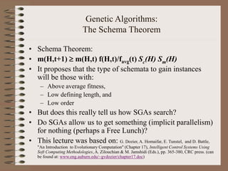
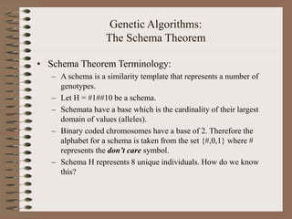
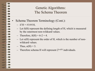
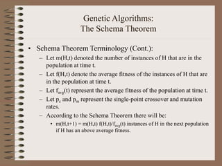
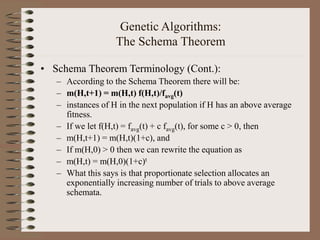
The Schema Theorem
• Schema Theorem Terminology (Cont.):
– m(H,t+1) = m(H,t) f(H,t)/favg(t)
– Although the above equation seems to say that above average
schemata are allowed an exponentially increasing number of
trials, instances may be gained or lost through the application of
single-point crossover and mutation.
– Thus we need to calculate the probability that schema H survives:
– Single-Point Crossover: Sc(H) =1- [pc (H)/(l-1)]
– Mutation: Sm(H) = (1- pm )o(H)

57. Genetic Algorithms:
The Schema Theorem
• Schema Theorem:
• m(H,t+1)  m(H,t) f(H,t)/favg(t) Sc(H) Sm(H)
• It proposes that the type of schemata to gain instances
will be those with:
– Above average fitness,
– Low defining length, and
– Low order
• But does this really tell us how SGAs search?
• Do SGAs allow us to get something (implicit parallelism)
for nothing (perhaps a Free Lunch)?
• This lecture was based on: G. Dozier, A. Homaifar, E. Tunstel, and D. Battle,
"An Introduction to Evolutionary Computation" (Chapter 17), Intelligent Control Systems Using
Soft Computing Methodologies, A. Zilouchian & M. Jamshidi (Eds.), pp. 365-380, CRC press. (can
be found at: www.eng.auburn.edu/~gvdozier/chapter17.doc)