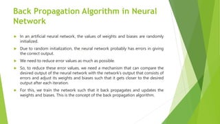
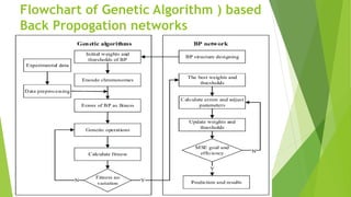
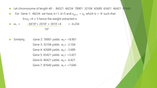
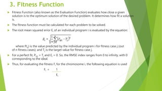
Genetic Algorithm Based Back
Propagation Network
Submitted By: Submitted To:
Rohit Poonia Dr.Linni Mathew
231516 (HOD & Professor, NITTTR)
Ravi Kumar Fulwaria
231515
Department of Electrical Engineering,
NITTTR Chandigarh
Content
 Genetic Algorithm
 Back Propagation network
 Genetic Algorithm based Back Propagation Network
 Coding
 Weight Extraction
 Fitness Factor
 Reproduction
 Convergence
 Conclusion
 References
Genetic Algorithm
 The Genetic Algorithm is a method for solving both constrained and
unconstrained optimization problems that is based on natural selection, the
process that drives biological evolution.
 The Genetic Algorithm repeatedly modifies a population of individual
solutions.
 At each step, the genetic algorithm selects individuals from the current
population to be parents and uses them to produce the children for the next
generation.
 Over successive generations, the population "evolves" toward an optimal
solution.
Flowchart of Genetic Algorithm
Back Propagation Algorithm in Neural
Network
 In an artificial neural network, the values of weights and biases are randomly
initialized.
 Due to random initialization, the neural network probably has errors in giving
the correct output.
 We need to reduce error values as much as possible.
 So, to reduce these error values, we need a mechanism that can compare the
desired output of the neural network with the network’s output that consists of
errors and adjust its weights and biases such that it gets closer to the desired
output after each iteration.
 For this, we train the network such that it back propagates and updates the
weights and biases. This is the concept of the back propagation algorithm.
Flowchart of Back
Propagation Algorithm
Genetic algorithm (GA) based Back
Propagation networks (BPN)
 Conventionally, a BPN determines its weights based on a gradient search
technique and therefore the risk of encountering the local minimum problem.
 GA on the other hand, though not guaranteed to find global optimum solution
to the problems but have been found to be good at finding “acceptably good”
solutions to problems at the quicker rate or use less number of iterations.
 The idea to hybridize the two approaches, namely Genetic Algorithm and
Backpropogation networks was given by Whitley , Bogart and Hanson in year
1990.
 They use GA to guide BPN in finding the optimal weights and to enhance the
speed of training.
Flowchart of Genetic Algorithm ) based
Back Propogation networks
Genetic Algorithm based Back
Propagation Network has 5 parts
1. Coding
2. Weight Extraction
3. Fitness Factor
4. Reproduction
5. Convergence
1.Coding
 Chromosomes: The parameters which represent a potential solution to the
problems, (genes) are joined together to form a string of values referred to as a
chromosomes.
 Assume a BPN whose network configuration is l-m-n ( l input neurons, m
hidden neurons and n output neurons).
 The number of weights that are to be determined are (l+n)*m.
 Let d = The number of digits in the weight
 Then String Length ,L = (l+n)*m*d is randomly generated
 The string S represents the weight matrices of the input-hidden and hidden-
output layers in a linear form.
 An initial population of “p” chromosomes is randomly generated where “p” is
referred as the “Population Size”
Example Of Coding:
 Consider a BPN network with configuration 3-2-1:
 l=3 input neurons, m=2 hidden neurons and n=1 output neurons
 The number of weights that are to be determined are (l+n)*m
= (3+1)*2= 8
 Let d = 5 The number of digits in the weight
 Then String Length ,L = (l+n)*m*d = 8*5=40 is randomly generated
2. Weight Extraction
 To determine the fitness values for each of the chromosomes, we extract weights from each of the
chromosomes.
 Let x1,x2,…….xd,……,..xL represents a chromosome and xkd+1, xkd+2,.. …….x(k+1)d
represent the kth gene (k≥0) in the chromosome.
 The actual weight wk is given by
+ xkd+210d-2+ xkd+310d-3 +……. x(k+1)d , if 5≤xkd+1≤ 9
 wk 10d-2
- xkd+210d-2+ xkd+310d-3 +……. x(k+1)d , if 0≤xkd+1≤ 5
10d-2
 Let chromosome of length 40 : 84321 46234 78901 32104 42689 63421 46421 87640
 For Gene 0: 84321 we have k=0, d=5 and xkd+1 = x1 which is = ‘8’ such that
5≤x1 =8 ≤ 9 hence the weight extracted is
w0 = + 4X10³+ 3X10² + 2X10 +1 = 4.321
103
 Let chromosome of length 40 : 84321 46234 78901 32104 42689 63421 46421 87640
 For Gene 1: 46234 we have, k=1, d=5 and xkd+1 = x6 which is = ‘4’ such that
0≤x6 =4 ≤ 5 hence the weight extracted is
 w1 = - 6X10³+ 2X10² + 3X10 +4 = -6.234
103
 Similarly, Gene 2: 78901 yields w2= +8.901
Gene 3: 32104 yields w3= -2.104
Gene 4: 42689 yields w4= -2.689
Gene 5: 63421 yields w5= +3.421
Gene 6: 46421 yields w6= -6.421
Gene 7: 87640 yields w7= +7.640
3. Fitness Function
 Fitness Function (also known as the Evaluation Function) evaluates how close a given
solution is to the optimum solution of the desired problem. It determines how fit a solution
is.
 The fitness function must be calculated for each problem to be solved.
 The root mean squared error Ei of an individual program i is evaluated by the equation:
where P(ij) is the value predicted by the individual program i for fitness case j (out
of n fitness cases); and Tj is the target value for fitness case j.
 For a perfect fit, P(ij) = Tj and Ei = 0. So, the RMSE index ranges from 0 to infinity, with 0
corresponding to the ideal.
 Thus, for evaluating the fitness Fi for the chromosome i, the following equation is used
Fi = 1
Ei
4. Reproduction
 In this phase the mating pool is first formed before the paranet chromosomes
reproduce to deliver offspring with better fitness.
 For the given problem the mating pool is first formed by excluding that chromosome
Ci with the least fitness Fmin and replacing it with a duplicate copy of the chromosome
Ck reporting the highest fitness Fmax.
 Now the best fit individuals have multiple copies while the worst fit individuals die off.
 From the mating pool the parents are selected in pairs at random
 The chromosomes of the respective pairs are recombined using the “Two point cross
over” operator of a standard GA
Two-Point Crossover
 This is a specific case of a N-point Crossover technique. Two random points
are chosen on the individual chromosomes (strings) and the genetic material
is exchanged at these points.
 The offspring which now form the current population again have their fitness
calculated as before by fitness function
5.Convergence
 For any problem, if the GA is correctly implemented, the population evolves over
successive generations with the fitness value increasing towards the global optimum
value.
 Convergence is the progression towards increasing uniformity.
 A population is said to have converged when 95% of the individuals constituting the
population share the same fitness value.
 The population P1 now undergoes the process of selection, reproduction and cross
over.
 The fitness values for the chromosomes in P1 are computed, the best individuals
replicated and reproduction carried out using two-point cross over operator to form
the next generation P2 of chromosomes.
 The process of generation proceeds until at one stage 95% of the chromosomes in the
population Pi converge to the same fitness value.
 At that stage the weights extracted from the population Pi are the final weights to be
used by the Back Propagation Network
Example
Limitations and Challenges
 Vanishing and Exploding Gradients: In very deep networks, gradients can
become very small (vanish) or very large (explode), making training difficult.
Techniques like LSTM in RNNs or ResNet in CNNs are used to mitigate this.
 Requirement of Differentiable Activation Functions: The activation functions
used in the network must be differentiable for backpropagation to work.
Thank You!!

GABPN genetic algorithm based back propogation networknew.pptx

  • 1.
    Genetic Algorithm BasedBack Propagation Network Submitted By: Submitted To: Rohit Poonia Dr.Linni Mathew 231516 (HOD & Professor, NITTTR) Ravi Kumar Fulwaria 231515 Department of Electrical Engineering, NITTTR Chandigarh
  • 2.
    Content  Genetic Algorithm Back Propagation network  Genetic Algorithm based Back Propagation Network  Coding  Weight Extraction  Fitness Factor  Reproduction  Convergence  Conclusion  References
  • 3.
    Genetic Algorithm  TheGenetic Algorithm is a method for solving both constrained and unconstrained optimization problems that is based on natural selection, the process that drives biological evolution.  The Genetic Algorithm repeatedly modifies a population of individual solutions.  At each step, the genetic algorithm selects individuals from the current population to be parents and uses them to produce the children for the next generation.  Over successive generations, the population "evolves" toward an optimal solution.
  • 4.
  • 5.
    Back Propagation Algorithmin Neural Network  In an artificial neural network, the values of weights and biases are randomly initialized.  Due to random initialization, the neural network probably has errors in giving the correct output.  We need to reduce error values as much as possible.  So, to reduce these error values, we need a mechanism that can compare the desired output of the neural network with the network’s output that consists of errors and adjust its weights and biases such that it gets closer to the desired output after each iteration.  For this, we train the network such that it back propagates and updates the weights and biases. This is the concept of the back propagation algorithm.
  • 6.
  • 7.
    Genetic algorithm (GA)based Back Propagation networks (BPN)  Conventionally, a BPN determines its weights based on a gradient search technique and therefore the risk of encountering the local minimum problem.  GA on the other hand, though not guaranteed to find global optimum solution to the problems but have been found to be good at finding “acceptably good” solutions to problems at the quicker rate or use less number of iterations.  The idea to hybridize the two approaches, namely Genetic Algorithm and Backpropogation networks was given by Whitley , Bogart and Hanson in year 1990.  They use GA to guide BPN in finding the optimal weights and to enhance the speed of training.
  • 8.
    Flowchart of GeneticAlgorithm ) based Back Propogation networks
  • 9.
    Genetic Algorithm basedBack Propagation Network has 5 parts 1. Coding 2. Weight Extraction 3. Fitness Factor 4. Reproduction 5. Convergence
  • 10.
    1.Coding  Chromosomes: Theparameters which represent a potential solution to the problems, (genes) are joined together to form a string of values referred to as a chromosomes.  Assume a BPN whose network configuration is l-m-n ( l input neurons, m hidden neurons and n output neurons).  The number of weights that are to be determined are (l+n)*m.  Let d = The number of digits in the weight  Then String Length ,L = (l+n)*m*d is randomly generated  The string S represents the weight matrices of the input-hidden and hidden- output layers in a linear form.  An initial population of “p” chromosomes is randomly generated where “p” is referred as the “Population Size”
  • 11.
    Example Of Coding: Consider a BPN network with configuration 3-2-1:  l=3 input neurons, m=2 hidden neurons and n=1 output neurons  The number of weights that are to be determined are (l+n)*m = (3+1)*2= 8  Let d = 5 The number of digits in the weight  Then String Length ,L = (l+n)*m*d = 8*5=40 is randomly generated
  • 12.
    2. Weight Extraction To determine the fitness values for each of the chromosomes, we extract weights from each of the chromosomes.  Let x1,x2,…….xd,……,..xL represents a chromosome and xkd+1, xkd+2,.. …….x(k+1)d represent the kth gene (k≥0) in the chromosome.  The actual weight wk is given by + xkd+210d-2+ xkd+310d-3 +……. x(k+1)d , if 5≤xkd+1≤ 9  wk 10d-2 - xkd+210d-2+ xkd+310d-3 +……. x(k+1)d , if 0≤xkd+1≤ 5 10d-2  Let chromosome of length 40 : 84321 46234 78901 32104 42689 63421 46421 87640  For Gene 0: 84321 we have k=0, d=5 and xkd+1 = x1 which is = ‘8’ such that 5≤x1 =8 ≤ 9 hence the weight extracted is w0 = + 4X10³+ 3X10² + 2X10 +1 = 4.321 103
  • 13.
     Let chromosomeof length 40 : 84321 46234 78901 32104 42689 63421 46421 87640  For Gene 1: 46234 we have, k=1, d=5 and xkd+1 = x6 which is = ‘4’ such that 0≤x6 =4 ≤ 5 hence the weight extracted is  w1 = - 6X10³+ 2X10² + 3X10 +4 = -6.234 103  Similarly, Gene 2: 78901 yields w2= +8.901 Gene 3: 32104 yields w3= -2.104 Gene 4: 42689 yields w4= -2.689 Gene 5: 63421 yields w5= +3.421 Gene 6: 46421 yields w6= -6.421 Gene 7: 87640 yields w7= +7.640
  • 14.
    3. Fitness Function Fitness Function (also known as the Evaluation Function) evaluates how close a given solution is to the optimum solution of the desired problem. It determines how fit a solution is.  The fitness function must be calculated for each problem to be solved.  The root mean squared error Ei of an individual program i is evaluated by the equation: where P(ij) is the value predicted by the individual program i for fitness case j (out of n fitness cases); and Tj is the target value for fitness case j.  For a perfect fit, P(ij) = Tj and Ei = 0. So, the RMSE index ranges from 0 to infinity, with 0 corresponding to the ideal.  Thus, for evaluating the fitness Fi for the chromosome i, the following equation is used Fi = 1 Ei
  • 15.
    4. Reproduction  Inthis phase the mating pool is first formed before the paranet chromosomes reproduce to deliver offspring with better fitness.  For the given problem the mating pool is first formed by excluding that chromosome Ci with the least fitness Fmin and replacing it with a duplicate copy of the chromosome Ck reporting the highest fitness Fmax.  Now the best fit individuals have multiple copies while the worst fit individuals die off.  From the mating pool the parents are selected in pairs at random  The chromosomes of the respective pairs are recombined using the “Two point cross over” operator of a standard GA
  • 16.
    Two-Point Crossover  Thisis a specific case of a N-point Crossover technique. Two random points are chosen on the individual chromosomes (strings) and the genetic material is exchanged at these points.  The offspring which now form the current population again have their fitness calculated as before by fitness function
  • 17.
    5.Convergence  For anyproblem, if the GA is correctly implemented, the population evolves over successive generations with the fitness value increasing towards the global optimum value.  Convergence is the progression towards increasing uniformity.  A population is said to have converged when 95% of the individuals constituting the population share the same fitness value.  The population P1 now undergoes the process of selection, reproduction and cross over.  The fitness values for the chromosomes in P1 are computed, the best individuals replicated and reproduction carried out using two-point cross over operator to form the next generation P2 of chromosomes.  The process of generation proceeds until at one stage 95% of the chromosomes in the population Pi converge to the same fitness value.  At that stage the weights extracted from the population Pi are the final weights to be used by the Back Propagation Network
  • 18.
  • 19.
    Limitations and Challenges Vanishing and Exploding Gradients: In very deep networks, gradients can become very small (vanish) or very large (explode), making training difficult. Techniques like LSTM in RNNs or ResNet in CNNs are used to mitigate this.  Requirement of Differentiable Activation Functions: The activation functions used in the network must be differentiable for backpropagation to work.
  • 20.
    Limitations and Challenges Vanishing and Exploding Gradients: In very deep networks, gradients can become very small (vanish) or very large (explode), making training difficult. Techniques like LSTM in RNNs or ResNet in CNNs are used to mitigate this.  Requirement of Differentiable Activation Functions: The activation functions used in the network must be differentiable for backpropagation to work.
  • 21.
    Limitations and Challenges Vanishing and Exploding Gradients: In very deep networks, gradients can become very small (vanish) or very large (explode), making training difficult. Techniques like LSTM in RNNs or ResNet in CNNs are used to mitigate this.  Requirement of Differentiable Activation Functions: The activation functions used in the network must be differentiable for backpropagation to work.
  • 22.
    Limitations and Challenges Vanishing and Exploding Gradients: In very deep networks, gradients can become very small (vanish) or very large (explode), making training difficult. Techniques like LSTM in RNNs or ResNet in CNNs are used to mitigate this.  Requirement of Differentiable Activation Functions: The activation functions used in the network must be differentiable for backpropagation to work.
  • 23.
    Limitations and Challenges Vanishing and Exploding Gradients: In very deep networks, gradients can become very small (vanish) or very large (explode), making training difficult. Techniques like LSTM in RNNs or ResNet in CNNs are used to mitigate this.  Requirement of Differentiable Activation Functions: The activation functions used in the network must be differentiable for backpropagation to work.
  • 24.
    Limitations and Challenges Vanishing and Exploding Gradients: In very deep networks, gradients can become very small (vanish) or very large (explode), making training difficult. Techniques like LSTM in RNNs or ResNet in CNNs are used to mitigate this.  Requirement of Differentiable Activation Functions: The activation functions used in the network must be differentiable for backpropagation to work.
  • 25.