Downloaded 49 times


![Equivalent Computers
z z zz z z z
1
Start
HALT
), X, L
2:
look
for (
#, 1, -
), #, R
(, #, L
(, X, R
#, 0, -
Finite State Machine
...
Turing Machine
term = variable
| term term
| (term)
| variable . term
y. M v. (M [y v])
where v does not occur in M.
(x. M)N M [ x N ]
Lambda Calculus
Functional Programming Computability](https://image.slidesharecdn.com/functionalbackground-150915104733-lva1-app6891/85/Computability-turing-machines-and-lambda-calculus-7-320.jpg)
![Alan Turing, 1936
• "On computable numbers, with an application
to the Entscheidungsproblem [decision
problem]”
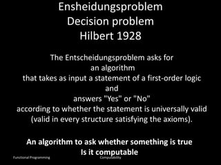
• addressed a previously unsolved
mathematical problem posed by the German
mathematician David Hilbert in 1928:
Functional Programming Computability](https://image.slidesharecdn.com/functionalbackground-150915104733-lva1-app6891/85/Computability-turing-machines-and-lambda-calculus-8-320.jpg)


![Equivalent Computers
z z zz z z z ...
Turing Machine
term = variable
| term term
| (term)
| variable . term
y. M v. (M [y v])
where v does not occur in M.
(x. M)N M [ x N ]
Lambda Calculus
Functional Programming Lambda Calculus](https://image.slidesharecdn.com/functionalbackground-150915104733-lva1-app6891/85/Computability-turing-machines-and-lambda-calculus-45-320.jpg)
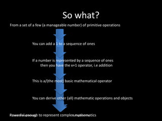
![What is Calculus?
• In High School:
d/dx xn = nxn-1 [Power Rule]
d/dx (f + g) = d/dx f + d/dx g [Sum Rule]
Calculus
is a branch of mathematics
that deals with limits
and the differentiation and
integration of functions
of one or more variables...
Functional Programming Lambda Calculus](https://image.slidesharecdn.com/functionalbackground-150915104733-lva1-app6891/85/Computability-turing-machines-and-lambda-calculus-46-320.jpg)


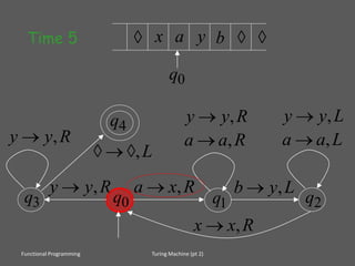
![Expression Reduction
Functional Programming Lambda Calculus
(𝛌x. x x) (𝛌y. y)
--> x x [𝛌y. y / x]
== (𝛌y. y) (𝛌y. y)
--> y [𝛌y. y / y]
== 𝛌y. y
How the original expression is
evaluated
Is determined the
operational semantics
of lambda calculus
(there are many ways to evaluate expressions)
Operational Semantics: how the substitutions are made:
Key concepts:
specification of free variables
specification of bound variables
Β-reduction
a formalization of simple substitution](https://image.slidesharecdn.com/functionalbackground-150915104733-lva1-app6891/85/Computability-turing-machines-and-lambda-calculus-57-320.jpg)


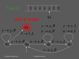
![Example
(λx. x x) (𝛌y. y)
--> x x [𝛌y. y / x]
== (𝛌y. y) (𝛌y. y)
--> y [𝛌y. y / y]
== 𝛌y. y
Substitute (𝛌y. y) into x
Substituted
Substitute (𝛌y. y) into y
Substituted
Functional Programming Examples](https://image.slidesharecdn.com/functionalbackground-150915104733-lva1-app6891/85/Computability-turing-machines-and-lambda-calculus-62-320.jpg)
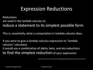
![Another example
(𝛌x. x x) (𝛌x. x x)
--> x x [𝛌x. x x/x]
== (𝛌x. x x) (𝛌x. x x)
In other words,
it is simple to write non terminating computations
in the lambda calculus
what else can we do?
Substitute 𝛌x. x x into every x
The result is the same as the beginning
Functional Programming Examples](https://image.slidesharecdn.com/functionalbackground-150915104733-lva1-app6891/85/Computability-turing-machines-and-lambda-calculus-63-320.jpg)

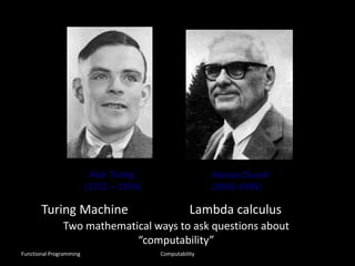
The document discusses functional programming and computability, focusing on concepts introduced by Alan Turing and Alonzo Church in the 1930s, including Turing machines and lambda calculus. It outlines the Entscheidungsproblem, which seeks algorithms to determine the truth of statements in first-order logic, and highlights Turing's assertion that there are well-defined problems that cannot be solved by computational procedures. The document further emphasizes the relationship between computation models and the Church-Turing thesis, asserting that both Turing machines and lambda calculus can compute the same functions.