Downloaded 71 times


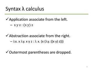

![Substitution
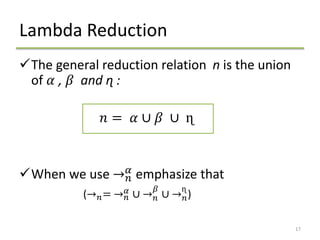
Substituting N for the free occurrences of x in M
Denoted by M[x := N]
x[x := N] ≡ N
y[x := N] ≡ y, if x ≠ y
(M1 M2)[x := N] ≡ (M1[x := N]) (M2[x := N])
(λx.M)[x := N] ≡ λx.M(λy.M)[x := N] ≡ λy.(M[x := N]), if x ≠ y, provided y ∉ FV(N)
12](https://image.slidesharecdn.com/lambdacalculus-160119180223/85/Lambda-Calculus-12-320.jpg)
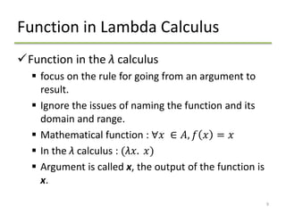
![Lambda Reduction
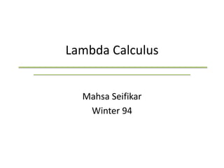
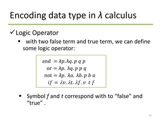
𝛼 − 𝑟𝑒𝑑𝑢𝑐𝑡𝑖𝑜𝑛
allows bound variable names to be changed.
if x and y is variable and M is a λ expression:
λx . M → 𝛼 λy . M[x → 𝑦]
Example :
λ𝑦 . λ𝑓 . 𝑓 𝑥 𝑦 → 𝛼 λ𝑧 . λ𝑓 . 𝑓 𝑥 𝑧
λ𝑧 . λ𝑓 . 𝑓 𝑥 𝑧 → 𝛼 λ𝑧 . λ𝑔 . 𝑔 𝑥 𝑧
13](https://image.slidesharecdn.com/lambdacalculus-160119180223/85/Lambda-Calculus-13-320.jpg)
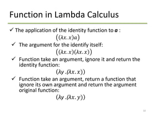
![Lambda Reduction
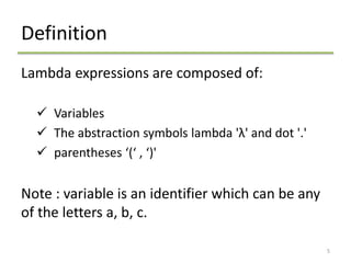
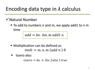
𝛽 − 𝑟𝑒𝑑𝑢𝑐𝑡𝑖𝑜𝑛
applying functions to their arguments.
If x is variable and M and N are λ expression:
( λ𝑥. 𝑀 ) 𝑁 → 𝛽 𝑀[ 𝑥 → 𝑁]
Example:
( ( λn . n∗x ) y) → y∗x
14](https://image.slidesharecdn.com/lambdacalculus-160119180223/85/Lambda-Calculus-14-320.jpg)


The document provides an extensive overview of lambda calculus, introduced by Alonzo Church in the 1930s as a formal model of computation. It covers its syntax, reduction methods, and application in functional programming languages, highlighting how various languages have implemented lambda calculus concepts. Additionally, it explains encoding data types and recursive functions in lambda calculus and discusses its implications for modern programming practices.


![[FLOLAC'14][scm] Functional Programming Using Haskell](https://cdn.slidesharecdn.com/ss_thumbnails/slides-140630030216-phpapp01-thumbnail.jpg?width=640&height=640&fit=bounds)