This paper presents a new algorithm called the translational propagation algorithm for generating near-optimal Latin hypercube designs (LHDs) without using formal optimization. The algorithm exploits patterns in optimal LHDs by translating small building blocks consisting of points within the design space. It was found that the algorithm represents a computationally fast strategy for obtaining good LHDs, especially for medium-dimensional design spaces. The algorithm divides the design space into blocks based on the number of points in the seed design and final LHD. It then propagates the seed design through translations to fill the blocks while maintaining Latin hypercube properties. Monte Carlo simulations evaluated the performance of the algorithm for different configurations and compared it to formal optimization approaches.

![136 F. A. C. VIANA, G. VENTER AND V. BALABANOV
computational crunch because of the ever increasing appetite for improved modeling of physical
processes and more detailed optimization [1]. To reduce the computational cost, surrogate models,
also known as meta-models, are often used in place of the actual simulation models [2–7].
Surrogate-based design optimization begins by identifying locations in the design space where
simulations will be conducted. This process of identifying locations in the design space is known
as design of experiments (DOE) [8, 9]. Response data (often via numerical simulations) are
collected at these locations and one or more candidate surrogate models are fitted to the data
[10–12]. Finally, one or more of the candidate models are selected for calculating responses (and
to facilitate objective and constraint calculation during the optimization process) at points in the
design space where the actual responses are not yet available.
It is well known among designers that the quality of fit, which often defines the performance
of the surrogate model during optimization and design space exploration, strongly depends on the
DOE (point location and density) [13, 14]. By quality of fit, the authors imply the discrepancy
(in a general sense) between the actual response and the value predicted by the corresponding
surrogate model. There exist many measures for the quality of fit, depending on the particular
problem under consideration [14, 15].
A DOE with n p points and n v variables is usually written as an n p ×n v matrix X =
[x1 , x2 , . . . , xn p ]T , where each row xi = [xi1 , xi2 , . . . , xinv ] represents a sample and each column
represents a variable. Within the design and analysis of computer experiments, the Latin hypercube
design (LHD) proposed by McKay et al. [16] and Iman and Conover [17] is very popular. The
LHD presents advantages such as (i) the number of samples (points) is not fixed; (ii) orthogonality
of the sampling points (a design is orthogonal if the inner product of any two columns is zero
[3, 18]); and (iii) the sampling points do not depend on the surrogate model that will be constructed.
An LHD with n p points is constructed in such a way that each of the n v variables is divided into
n p equal levels and that there is only one point (or sample) at each level. A random procedure
is used to determine the point locations. Figure 1 shows two examples of LHDs with n v = 2 and
n p = 16. As the LHD is constructed using a random procedure, there is nothing preventing a
design that has poor space filling qualities, as the extreme case illustrated in Figure 1(a). A better
choice is shown in Figure 1(b), where the points are more uniformly distributed in the domain.
The optimization of the space-filling qualities of the LHD is a challenging problem that has
resulted in a number of research publications [19–28]. One interpretation of the space-filling
property is to consider a n v -dimensional sphere around each design point in the experimental
design. The larger the radius of the smallest sphere that does not cross the boundary of the design
space, the better the space-filling property of the design. Optimizing the point location in a LHD to
Figure 1. Examples of Latin hypercube designs: (a) ill-suited LHD with n v = 2 and n p = 16 and
(b) reasonable LHD with n v = 2 and n p = 16.
Copyright q 2009 John Wiley & Sons, Ltd. Int. J. Numer. Meth. Engng 2010; 82:135–156
DOI: 10.1002/nme](https://image.slidesharecdn.com/fulltext-100505081143-phpapp01/85/Fulltext-2-320.jpg)
![AN ALGORITHM FOR FAST OPTIMAL LHD 137
Table I. Approaches for constructing the optimal Latin hypercube design.
Researchers Year Algorithm Objective functions
Audze and Egl¯ js [19]
a 1977 Coordinates Exchange Potential energy
Algorithm
Park [20] 1994 A 2-stage (exchange- and Integrated mean-squared error
Newton-type) algorithm and entropy criteria
Morris and Mitchell [21] 1995 Simulated annealing
p criterion
Ye et al. [22] 2000 Columnwise–pairwise
p and entropy criteria
Fang et al. [23] 2002 Threshold accepting algorithm Centered L 2 -discrepancy
Bates et al. [24] 2004 Genetic algorithm Potential energy
Jin et al. [25] 2005 Enhanced stochastic
p criterion, entropy and L 2
evolutionary algorithm discrepancy
Liefvendahl and Stocki [26] 2006 Columnwise-pairwise and Minimum distance and
genetic algorithms Audze–Egl¯ js functions
a
van Dam et al. [27] 2007 Branch-and-bound algorithm 1-norm and infinite norm
distances
Grosso et al. [28] 2008 Iterated local search and
p criterion
simulated annealing
algorithms
improve the uniformity of the point distribution, typically by maximizing the radius of the smallest
sphere, results in an Optimal LHD. Such designs are usually obtained from time-consuming
combinatorial optimization problems, with search space of the order of (n p !)n v . For example, to
optimize the location of 20 samples in two dimensions, the algorithm has to select the best design
from more than 1036 possible designs. If the number of variables is increased to 3, the number
of possible designs is more than 1055 . Researches have proposed various optimization algorithms
and objective functions to solve this problem. Table I summarizes some strategies found in the
literature. As for the computational time, Ye et al. [22] reported several hours on a Sun SPARC
20 workstation for generating an optimal Latin hypercube with 25 points for 4 variables. Jin et al.
[25] reported minutes on a PC with a Pentium III 650 MHZ CPU for generating an optimal Latin
hypercube with 100 points for 10 variables. Section 4 shows a comparison of different optimization
methods for obtaining optimal LHDs with contemporary computing power.
Owing to its popularity, the
p criterion was selected as a performance measure in this paper.
Minimizing
p leads to the maximization of the point-to-point distance in the design (see [21, 25]
for details). Mathematically:
n p −1 np 1/ p
−p
p = dij (1)
i=1 j=i+1
where p is a positive integer, n p is the number of points in the design, and dij is the inter-point
distance between all point pairs in the design. The general interpoint distance between any point
pair xi and x j can be expressed as follows:
nv 1/t
dij = d(xi , x j ) = |xik − xjk |t , t = 1 or 2 (2)
k=1
In the present work, p = 50 and t = 1 are used following the suggestions of Jin et al. [25].
Copyright q 2009 John Wiley & Sons, Ltd. Int. J. Numer. Meth. Engng 2010; 82:135–156
DOI: 10.1002/nme](https://image.slidesharecdn.com/fulltext-100505081143-phpapp01/85/Fulltext-3-320.jpg)


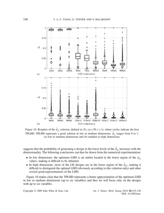
![AN ALGORITHM FOR FAST OPTIMAL LHD 145
Table II. Latin hypercube design configurations considered.
No. of points
No. of variables Small designs Medium designs Large designs
2 12 20 120
4 30 70 300
6 56 168 560
8 90 330 900
10 132 572 1320
12 182 910 1820
compared using the values of the
p criterion. Next, the efficiency of the proposed algorithm
in approximating the optimal LHD was studied. For this study, an estimate of the range of the
p criterion for the LHDs proposed in Table II is created based on Monte Carlo simulation plus
the results from 100 simulations of three different Latin Hypercube optimization techniques. The
Monte Carlo simulation created 200 000 random LHDs for the configurations proposed in Table II
(this is possible because the Latin hypercube algorithm allows for the creation of different designs
based on a random number generator). The three different Latin Hypercube optimization techniques
used in the study are:
1. The Enhanced Stochastic Evolutionary algorithm (ESEA) of Jin et al. [25]: set with maximum
number of 20 iterations (but each simulation was allowed to run at most five iterations without
improvement of the objective function).
2. The Genetic algorithm (GA) implementation of Bates et al. [24]: set with maximum number
of 50 iterations (but each simulation was allowed to run at most 20 iterations without
improvement of the objective function).
3. The native MATLAB function lhsdesign [29]: using the maxmin criterion (maximization
of the minimum distance) and 200 iterations. With these settings, the MATLAB lhsdesign
function selects the best LHD from 200 randomly created designs. The maxmin criterion is
used to select the best design.
The settings for both GA and ESEA were based on a few trials for the design with 560
points and 6 variables. All simulations were conducted using an Intel Core 2 Quad CPU Q6600
at 2.40 GHz, with 3 GB of RAM running MATLAB 7.6 (R2008a) under Windows XP. The
SURROGATES toolbox [30] was used to execute the TPLHD, ESEA, and GA algorithms under
MATLAB [29].
˜
Instead of showing only the
p criterion as defined in Equation (1), a normalized version,
p ,
is also presented for easier comparison:
p −min(
p )
˜
p = (5)
max(
p )−min(
p )
where max(
p ) and min(
p ) are the maximum and minimum values of
p found in the generated
˜
DOEs (including both the TPLHDs and the Monte Carlo simulations); which means that 0
p 1.
Using the Monte Carlo simulations and the optimization results, it is possible to estimate the
range of variation of
p values and thus make a judgment if a specific design represents a
Copyright q 2009 John Wiley & Sons, Ltd. Int. J. Numer. Meth. Engng 2010; 82:135–156
DOI: 10.1002/nme](https://image.slidesharecdn.com/fulltext-100505081143-phpapp01/85/Fulltext-11-320.jpg)


![AN ALGORITHM FOR FAST OPTIMAL LHD 149
Table V. Performance comparison between TPLHD and the median out of 100 simulations of different
optimization techniques. ESEA is the implementation of the Enhanced Stocastic Evolutionary algorithm of
Jin et al. [25]. lhsdesign is a native MATLAB function. GA refers to the Genetic algorithm implementation
˜
of Bates et al. [24].
p , defined in (5), ranges from 0 to 1.
No. of variables 2 4 6
No. of points 12 20 120 30 70 300 56 168 560
˜
p TPLHD 0.1 0.1 0 0 0 0 0.1 0 0
ESEA 0.2 0.1 0.1 0 0 0 0 0 0
GA 0.2 0.3 0.3 0.1 0.1 0 0 0 0
lhsdesign 0.5 0.5 0.6 0.1 0.1 0.1 0.1 0.0 0.1
Time (s) TPLHD ∼0
= ∼0
= 0.1 ∼0
= ∼0
= 0.7 ∼0
= 0.5 2
ESEA ∼0
= 0.2 13 0.3 3 173 2 34 1096
GA 0.4 0.9 24 4 17 275 19 143 1509
lhsdesign ∼0
= ∼0
= 0.2 ∼0
= 0.1 1.8 0.1 1.0 13
Table V allows a comparison between the TPLHD and the mean out of 100 simulations of three
different optimization techniques: (i) the ESEA of Jin et al. [25]; (ii) the GA implementation of
Bates et al. [24]; and (iii) the native MATLAB function lhsdesign [29]. TPLHD was obtained
by generating five candidates from different seeds and then picking the best one according to the
p criterion (which means that Table V shows the time needed to generate all five candidates.
Appendix B shows the discussion on the number of points that needs to be allocated in each of the
cases; which directly impacts the computational cost). Results in Table V reinforce that TPLHD
˜
offers very good solutions; with most of the designs presenting
p = 0. This means that TPLHD
found the best result of the set of all simulations (including the Monte Carlo and all optimization
ones). As for the computational cost, the TPLHD design is superior in most of the cases or in
the worst-case matches the best time of the traditional optimization techniques. Clearly, the point
density has a dramatic impact on the optimization techniques (especially ESEA and GA). For
instance, for the ESEA with 6 variables, moving from 56 to 560 points makes the computational
cost change from 2 s to a little more than 18 min. The lhsdesign MATLAB function tends to suffer
less, as it can be seen as a Monte Carlo simulation with only 200 samples (200 is the number of
iterations that lhsdesign was allowed to run). Still, in six dimensions, when moving from 56 to
560 points the computational cost of the lhsdesign increases more than 100 times.
Table V gives the impression that increasing the number of variables (no matter the point density)
made the three optimization techniques to improve their own performance (in terms of the
p ˜
˜
criterion). Considering the
p criterion of the designs with four and six variables, TPLHD and any
of the optimization techniques would offer designs that are below 0.1. Then, the computational
cost would leave only TPLHD and the lhsdesign as competing strategies. However, a closer look at
˜
the distributions of the
p criterion shows that TPLHD is the best choice. Figure 11 contrasts the
˜
box plot of the
p criterion with the values found by TPLHD and the 0.1 threshold of lhsdesign.
Because the distributions tend to lower values, the 0.1 threshold is a bad value for the 300×4
design and is a marginal to undesired value in 6 dimensions. It is clear that TPLHD offers a better
design (not mentioning a faster solution).
Copyright q 2009 John Wiley & Sons, Ltd. Int. J. Numer. Meth. Engng 2010; 82:135–156
DOI: 10.1002/nme](https://image.slidesharecdn.com/fulltext-100505081143-phpapp01/85/Fulltext-15-320.jpg)
![150 F. A. C. VIANA, G. VENTER AND V. BALABANOV
˜
Figure 11. Boxplots of the
p criterion between 0 and 0.5 for the four and six-dimensional designs.
˜
is defined in (5), ( p = 50, t = 1) and ranges from 0 to 1. Circles indicate the TPLHD.
p
One of the reasons for the poor performance of the TPLHD in high dimensions might be the
existence of the directionality property of TPLHD. Because of the way the points are created in
TPLHD, they tend to be stretched along one direction. Even the optimal LHD (obtained with
ESEA or GA for example) from Figure 1(b) may be considered as having points placed in a
preferred direction (close to 45◦ ). Goel et al. [14] discussed that a single criterion for generating
DOE may lead to large deteriorations in other criteria. In the proposed algorithm, the
p criterion
is used and the directionality of the resulting LHDs (for both the TPLHD and the designs obtained
with traditional optimization) is a clear loss. There has been work on the optimization of the
space-filling properties of the LHD while preserving low correlation between variables. Cioppa and
Lucas [31] presented an algorithm that improves the space-filling properties of LHD at the expense
of inducing small correlations between the columns in the design matrix. However, authors warned
that the approach is computationally prohibitive. Hernandez [32] presented an extensive study on
a set of methodologies to create design matrices with little or no correlation (including saturated
nearly orthogonal LHDs). Franco et al. [33] discussed a radar-shaped statistic for identifying
the directionality property in a DOE (especially efficient in low dimension). However, there
has been little research on how to employ this statistic for improving DOE and not just for
identifying the directionality in an existing DOE, the directionality statistic was not employed to
improve existing DOE in this paper. Nevertheless, the focus of this research is the translational
propagation algorithm as a cheap alternative to traditional optimization of the LHDs based on the
p criterion.
Other, more general questions arise in higher dimensions: it is not clear what is the meaning
of space-filling designs and the relative cost of any optimization strategy of experimental designs.
The sparsity of the data may make it difficult to judge whether designs given by the optimization
of the Latin hypercube are in fact space-filling designs. Even if they are, considering plots such
as those in Figure 10, the computational cost of strategies such as TPLHD may end up being
very close to random search (such as in lhsdesign). It may happen that in higher dimensions it
is not worth investing much in time-consuming optimization (few iterations of random search
Copyright q 2009 John Wiley & Sons, Ltd. Int. J. Numer. Meth. Engng 2010; 82:135–156
DOI: 10.1002/nme](https://image.slidesharecdn.com/fulltext-100505081143-phpapp01/85/Fulltext-16-320.jpg)


![154 F. A. C. VIANA, G. VENTER AND V. BALABANOV
Table AIV. MATLAB implementation of the resizeTPLHD function. ones(m, n) is the MATLAB function
that creates an m-by-n matrix of ones. zeros(m, n) is the MATLAB function that creates an m-by-n
matrix of zeros. norm(x) is the MATLAB function that computes the vector norm ( (xi2 )). min (x)
is the MATLAB function that finds the smallest element in x. sort(a) is the MATLAB function that
sorts the vector a in the ascending order, returning the sorted and the index vectors. sortrows(X, COL)
is the MATLAB function that sorts the matrix X based on the columns specified in the vector COL.
isequal(A, B) is the MATLAB function that returns logical 1 (TRUE) if arrays A and B are the same size
and contain the same values, and logical 0 (FALSE) otherwise.
1: function X = resizeTPLHD(X, npStar, np, nv)
2: % inputs: X - initial Latin hypercube design
3: % npStar - number of points in the initial X
4: % np - number of points in the final X
5: % nv - number of variables
6: % outputs: X - final X, properly shrunk
7:
8: center = npStar*ones(1,nv)/2; % center of the design space
9: % distance between each point of X and the center of the design space
10: distance = zeros(npStar, 1);
11: for c1 = 1 : npStar
12: distance(c1) = norm( ( X(c1,:) - center) );
13: end
14: [dummy, idx] = sort(distance);
15: X = X( idx(1:np), : ); % resize X to np points
16:
17: % re-establish the LH conditions
18: Xmin = min(X);
19: for c1 = 1 : nv
20: % place X in the origin
21: X = sortrows(X, c1);
22: X(:,c1) = X(:,c1) - Xmin(c1) + 1;
23: % eliminate empty coordinates
24: flag = 0;
25: while flag == 0;
26: mask = (X(:,c1) ∼ = ([1:np]’));
27: flag = isequal(mask,zeros(np,1));
28: X(:,c1) = X(:,c1) - (X(:,c1) ∼ = ([1:np]’));
29: end
30: end
31: return
the call for the function that creates the initial LHD. If necessary, the design is then resized to
the initially set configuration. Table AII gives the implementation of the reshaping of the seed
design (see Section 2.3). Table AIII illustrates the body of the translational propagation algorithm.
Lines 16–18 show how to create the displacement vector that is used to translate the seed in the
hyperspace. Finally, Table AIV presents the implementation of the resizing process. Lines 8–15
show how we reduce the initially large Latin hypercube to the n p initially set. Lines 18–30 present
how to restore the Latin hypercube condition of one point per level to the remaining points.
Copyright q 2009 John Wiley & Sons, Ltd. Int. J. Numer. Meth. Engng 2010; 82:135–156
DOI: 10.1002/nme](https://image.slidesharecdn.com/fulltext-100505081143-phpapp01/85/Fulltext-20-320.jpg)


![[AAAI-16] Tiebreaking Strategies for A* Search: How to Explore the Final Fron...](https://cdn.slidesharecdn.com/ss_thumbnails/2016215aaai-160217025704-thumbnail.jpg?width=640&height=640&fit=bounds)