The document covers the principles of fluid statics, focusing on pressure concepts, hydrostatic pressure distribution, and pressure measurement techniques. It elaborates on important concepts such as Pascal's law, gauge pressure, and various manometers and their applications, including limitations and examples for practical understanding. The material provides a solid foundation for understanding stationary fluids and pressure calculations in different scenarios.

1. 1
Akshoy Ranjan Paul
Associate Professor
Email: arpaul2k@gmail.com
DEPARTMENT OF APPLIED MECHANICS
MOTI LAL NEHRU NATIONAL INSTITUTE OF
TECHNOLOGY ALLAHABAD
Fluid Mechanics and Hydraulic
Machines (AMN13104)
B Tech. Mechanical Engg. (3rd semester)
Chapter-2: Fluid Statics

2. Chapter 2: Fluid Statics
2

3. Pressure concepts and problems
3

4. 4
Force Equilibrium of a Fluid
Element
• Fluid static is a term that is referred to the state of a
fluid where its velocity is zero and this condition is also
called hydrostatic.
• So, in fluid static, which is the state of fluid in which the
shear stress is zero throughout the fluid volume.
• In a stationary fluid, the most important variable is pressure.
• For any fluid, the pressure is the same regardless its direction.
As long as there is no shear stress, the pressure is independent
of direction. This statement is known as Pascal’s law

5. Force Equilibrium of a Fluid
Element Fluid surfaces
Figure 2.1 Pressure acting uniformly in all directions
Figure 2.2: Direction of fluid pressures on boundaries 5

6. Force Equilibrium of a Fluid
Element
Pressure is defined as the amount of surface force exerted by
a fluid on any boundary it is in contact with. It can be written
as:
•
•
•
Unit: N / m2 or Pascal (Pa).
(Also frequently used is bar, where 1 bar = 105 Pa).
(2.1)
A
Area of which the force is
applied
Force
P 
F
Pressure

6

7. Force Equilibrium of a Fluid
Element
• The formulation for pressure gradient can be written
as:
• p = (g –
a)
(2.11)
•
•
1. If a = 0, the fluid is stationary.
2. if a ≠ 0, the fluid is in the rigid body motion.
• The formulation for pressure gradient in Eq. (2.11) is derived under the
assumption that there is no shear stress present, or in other word, there
is no viscous effect.
• The rest of this chapter will only concentrate on the first case, i.e.
stationary fluids. The second case is applicable the case for a fluid in a
container on a moving platform, such as in a vehicle, and is out of scope
of this course. 7

8. Hydrostatic Pressure
Distribution
•For a liquid, usually the position is measured as distance from the
free surface, or depth h, which is positive downward as illustrated in
Fig. 2.3. Hence,
•
•
p2 – p1 = g (h2 – h1) =  (h2 –
h1)
p = g h =  h
8

9. Hydrostatic Pressure
Distribution
 If the atmospheric pressure p0 is taken as reference and is calibrated
as zero, then p is known as gauge pressure. Taking the pressure at
the surface as atmospheric pressure p0, i.e., p1=p, p2=p0 when
h1=h, h2=0, respectively:
p = p0 + gh = p0 + h
 This equation produces a linear, or uniform, pressure distribution
with depth and is known hydrostatic pressure distribution.
 The hydrostatic pressure distribution also implies that pressure is
the same for all positions of the same depth.
9

10. Hydrostatic Pressure
Distribution
• This statement can be explained by using a diagram in Fig. 2.4, where all
points, a, b, c and d, have the same value of pressure, that is
• pa = pb = pc = pd
• However, the pressure at point D is not identical from those at points, A,
B, and C since the fluid is different, i.e.
• pA = pB = pB ≠ pD
10

11. Standard
Atmosphere
 A pressure is quoted in its gauge value, it usually refers to a standard
atmospheric pressure p0. A standard atmosphere is an idealised
representation of mean conditions in the earth’s atmosphere.
 Pressure can be read in two different ways; the first is to quote the
value in form of absolute pressure, and the second to quote relative
to the local atmospheric pressure as reference.
 The relationship between the absolute pressure and the gauge
pressure is illustrated in Figure 2.6.
11

12. Standard Atmosphere
 The pressure quoted by the latter approach (relative to the local atmospheric
pressure) is called gauge pressure, which indicates the ‘sensible’ pressure since this
is the amount of pressure experienced by our senses or sensed by many pressure
transducers.
 If the gauge pressure is negative, it usually represent suction or partially
vacuum. The condition of absolute vacuum is reached when only the pressure
reduces to absolute zero.
12

13. Pressure
Measurement
 Based on the principle of hydrostatic pressure distribution, we can develop
an
apparatus that can measure pressure through a column of fluid (Fig. 2.7)
13

14. Pressure
Measurement
 We can calculate the pressure at the bottom surface which has to
withstand the weight of four fluid columns as well as the atmospheric
pressure, or any additional pressure, at the free surface. Thus, to find p5,
Total fluid columns = (p2 – p1) + (p3 – p2) + (p4 – p3) + (p5 – p4)
p5 – p1 = og (h2 – h1) + wg (h3 – h2) +
gg (h4 – h3) + mg (h5 – h4)
 The p1 can be the atmospheric pressure p0 if the free surface at z1 is
exposed to atmosphere. Hence, for this case, if we want the value in
gauge pressure (taking p1=p0=0), the formula for p5 becomes
p5 = og (h2 – h1) + wg (h3 – h2) + gg (h4 – h3) + mg (h5 – h4)
 The apparatus which can measure the atmospheric pressure is called
barometer (Fig 2.8).
14

15. Pressure Measurement
 For mercury (or Hg — the chemical symbol for mercury), the height
formed
is 760 mm and for water 10.3 m.
patm = 760 mm Hg (abs) = 10.3 m water (abs)
 By comparing point A and point B, the atmospheric pressure in the SI unit,
Pascal,
pB = pA + gh
pacm
= pv + gh
= 0.1586 + 13550 (9.807)(0.760)
 101 kPa
15

16. Pressure
Measurement
 This concept can be extended to general pressure measurement using an apparatus
known as manometer. Several common manometers are given in Fig. 2.9. The
simplest type of manometer is the piezometer tube, which is also known as ‘open’
manometer as shown in Fig. 2.9(a). For this apparatus, the pressure in bulb A can be
calculated as:
pA = p1 + p0
= 1gh1 + p0
 Here, p0 is the atmospheric pressure.
If a known local atmospheric pressure
value is used for p0, the reading for pA
is in absolute pressure. If only the
gauge pressure is required, then p0 can
be taken as zero.
16

17. Pressure
Measurement
 Although this apparatus (Piezometer) is simple, it has limitations, i.e.
a) It cannot measure suction pressure which is lower than the atmospheric
pressure,
b) The pressure measured is limited by available column height,
c) It can only deal with liquids, not gases.
 The restriction possessed by the piezometer tube can be overcome by the U-
tube manometer, as shown in Fig. 2.9(b). The U-tube manometer is also an
open manometer and the pressure pA can be calculated as followed:
p2 = p3
pA + 1gh1 = 2gh2 + p0
 pA
= 2gh2 - 1gh1 +
p0
17

18. Pressure
Measurement
 If fluid 1 is gas, further simplification can be made since it can be assumed that
1   2, thus the term 1gh1 is relatively very small compared to 2gh2 and
can be
omitted with negligible error. Hence, the gas pressure is:
pA  p2 = 2gh2 - p0
 There is also a ‘closed’ type of manometer as shown in Fig. 2.9(c), which can
measure pressure difference between two points, A and B. This apparatus is known
as the differential U-tube manometer. For this case, the formula for pressure
difference can be derived as followed:
p2 = p3
pA + 1gh1 = pB + 3gh3 + 2gh2
 pA - pB = 3gh3 + 2gh2 - 1gh1
18

19. Example
2.5
•An underground gasoline tank is accidentally opened during raining causing
the water to seep in and occupying the bottom part of the tank as shown in
Fig. E2.1. If the specific gravity for gasoline 0.68, calculate the gauge
pressure at the interface of the gasoline and water and at the bottom of the
tank. Express the pressure in Pascal and as a pressure head in metres of
water. Use water = 998 kg/m3 and g = 9.81 m/s2.
19

20. •For gasoline:
• g = 0.68(998) = 678.64kg/m3
At the free surface, take the atmospheric pressure to be zero, or p0 = 0 (gauge
pressure).
•
•
p1 = p0 + pgghg = 0 + (678.64)(9.81)(5.5)
= 36616.02 N/m2 = 36.6 kPa
•The pressure head in metres of water is:
h1 = p1 – p0 = 36616.02 - 0
pwg (998)
(9.81)
•
•
• = 3.74 m of water
•At the bottom of the tank, the pressure:
•
•
p2 = p1 + pgghg = 36616.02 + (998)(9.81)(1)
= 46406.4 N/m2 = 46.6 kPa
•And, the pressure head in meters of water is:
h2 = p1 – p0 = 46406.4 - 0
pwg (998)(9.81)
•
•
• = 4.74 m of water
Example
2.5
20

21. • Example 2.6
 Figure below shows a tank with one side open to the
atmosphere and the other side sealed with air above the oil
(SG=0.90). Calculate the gauge pressure at points
A,B,C,D,E.
2 m
3 m
1 m
E
A
C
B D
Oil (SG = 0.90)
21

22. Example 2.6
• Solution:
Thus PB = PA +
oilgh
= 0 + 0.9x1000x9.81x3
= 26.5 kPa (gauge)
Point C is 5 m below point A,
Thus PC = PA +
oilgh
= 0 + 0.9x1000x9.81x5
= 44.15 kPa (gauge)
Point D is at the same level of point B,
thus PD = PB
= 26.5 kPa (gauge)
Point E is higher by 1 m from point A,
• At point A, the oil is exposed to the atmosphere
• thus PA=Patm = 0 (gauge)
• Point B is 3 m below point A,
•
•
•
•
•
•
•
•
•
•
•
•
•
•
Thus PE = PA -
oilgh
= 0 - 0.9x1000x9.81x1
= -8.83 kPa (gauge).
22

23. 23
•
(same horizontal level)
We know that P2 = P3
•Thus

• Hggh2 = PA +
waterg(h1+h2)
•
•
•
•
•
PA = Hggh2 - waterg(h1+h2)
PA = 13.54x1000x9.81x0.3 – 1000x9.81x(0.2+0.3)
PA = 39, 848 - 4905
PA = 34.9 kPa (gauge)
Points to be selected:
1 – at the open end of the
manometer 2 – at the right leg of
the manometer 3 – same level with
point 2 but at left
leg of the manometer
4 – same level as point
A
Pressure at the
points: P1=Patm
P2 = P3
P4 = PA
A
•Example 2.7
•Determine the pressure at point A in the figure below if
h1 = 0.2 m and h2 = 0.3 m. Use water = 1000 kg/m3.
•Solution:
• P2 = P1 + Hggh2
•But P1 = Patm (open to atmosphere) ==>P1 = 0 (gauge)
•  P2 = Hggh2
• P3 = PA + waterg(h1+h2)

24. Micromanometer
The micro manometers are used for measuring small pressure difference.
The micro manometers utilizes two manometric liquids, which are
immiscible with each other and also with the fluid whose pressure
difference is to be measured.
When PA > PB , the liquid levels will be as shown in fig.
The volume of the liquid displaced in each tank is equal to the volume of
liquid displaced in the U-tube.
If a= cross-sectional area of the U-tube and A= cross-sectional area of tank
then,
Az  h/ 2a
24

25. 25

26. 26

27. • Example 2.8
 A 6-m deep tank contains 4 m of water and 2-m of oil as
shown in the diagram below. Determine the pressure
at point A and at the bottom of the tank. Draw the
pressure diagram.
A
oil
water
2 m
4 m
water = 1000 kg/m3
SG of oil = 0.98
27

28. Solution:
Pressure at oil water interface (PA)
PA = Patm + Poil (due to 2 m of oil)
= 0 + oilghoil = 0 + 0.98 x 1000 x 9.81 x
2
= 15696 Pa
PA = 15.7 kPa (gauge)
Pressure at the bottom of the tank;
PB = PA + waterghwater
PB = 15.7x1000 + 1000 x 9.81 x 4
= 54940 Pa
PB = 54.9 kPa (gauge)
Patm = 0
4 m
2 m
PA
PA=15.7 kPa
B
A
oil
water
PB = 54.9 kPA
Pressure Diagram
28

29. Hydrostatic forces
29

30. Figure 3.1 (p. 31)
Pressure is a scalar quantity
Force balance in the x-direction:
PASCAL’S LAW
30

31. Force balance in the z-direction:
Vertical force on
A
Vertical force on
lower boundary
Total weight of wedge element
31
= specific weight

32. From last slide:
Divide through by to get
Now shrink the element to a point:
This can be done for any orientation ,
so
32

33. Pressure Variation with Elevation
Figure 3.4 (p. 35)
Static fluid:
All forces must balance as there
are no accelerations.
Look at force balance in
direction of  l
33

34. From figure, note that
Shrink cylinder to zero
length:
(from previous slide)
34
or

35. Hydrostatic
Forces
 If a solid plate is immersed into the fluid, the pressure is
also acted upon the surface of the solid.
 This pressure acts on the submerged area thus generating
a kind of resultant force known as hydrostatic force.
 Hence, the hydrostatic force is an integration of fluid
pressure on an area.
 Similar to pressure, the direction in which the force
is acting is always perpendicular to the surface.
 To derive the hydrostatic force for a planar
 To derive the hydrostatic force for a planar surface,
consider the solid plate shown in following slide..
35

36. 36

37. 37

38. 38

39. 39

40. 40

41. 41

42. CONTINUE…….
42

43. 43

44. CONTINUE…….
44

45. 45

46. Example
2.1
 A circular door having a diameter of 4 m is positioned at the inclined wall as
shown in Fig. E2.3(a), which forms part of a large water tank. The door is
mounted on a shaft which acts to close the door by rotating it and the door is
restrained by a stopper. If the depth of the water is 10 m at the level of the shaft,
Calculate:
(a) Magnitude of the hydrostatic
force acting on the door and its
center of pressure,
(b) The moment required by the
shaft to open the door.
Use  water = 1000 kg/m3
and
g = 9.81 m/s2.
46

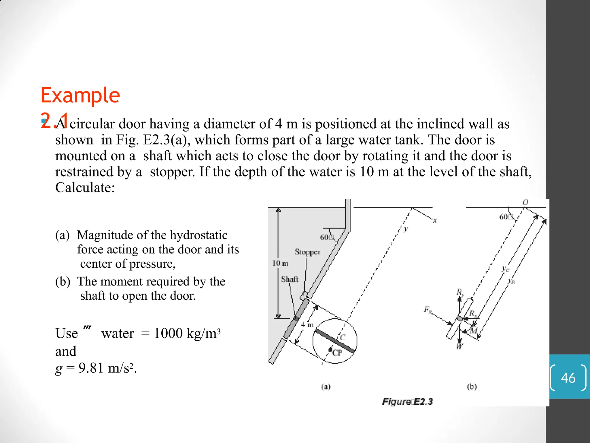
47. (a) The magnitude of the hydrostatic force FR is
FR = ghC A
= (998)(9.81)(10) [ ¼ x(4)2]
= 1.230 x 106 N
= 1.23 MN
For the coordinate system shown in Figure E2.3(b), since circle is a
symmetrical shape, Ixy = 0, then xR = 0. For y coordinate,
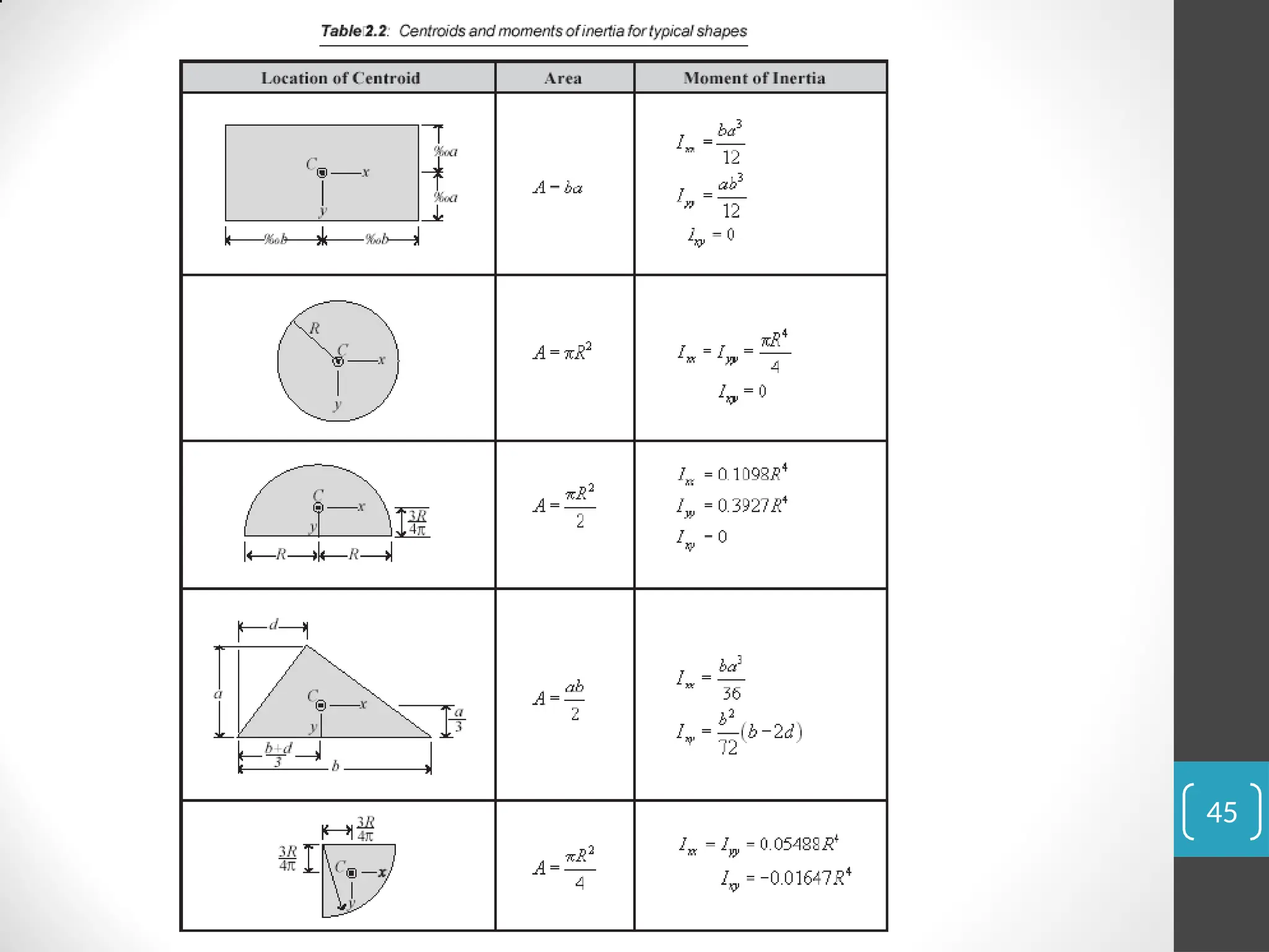
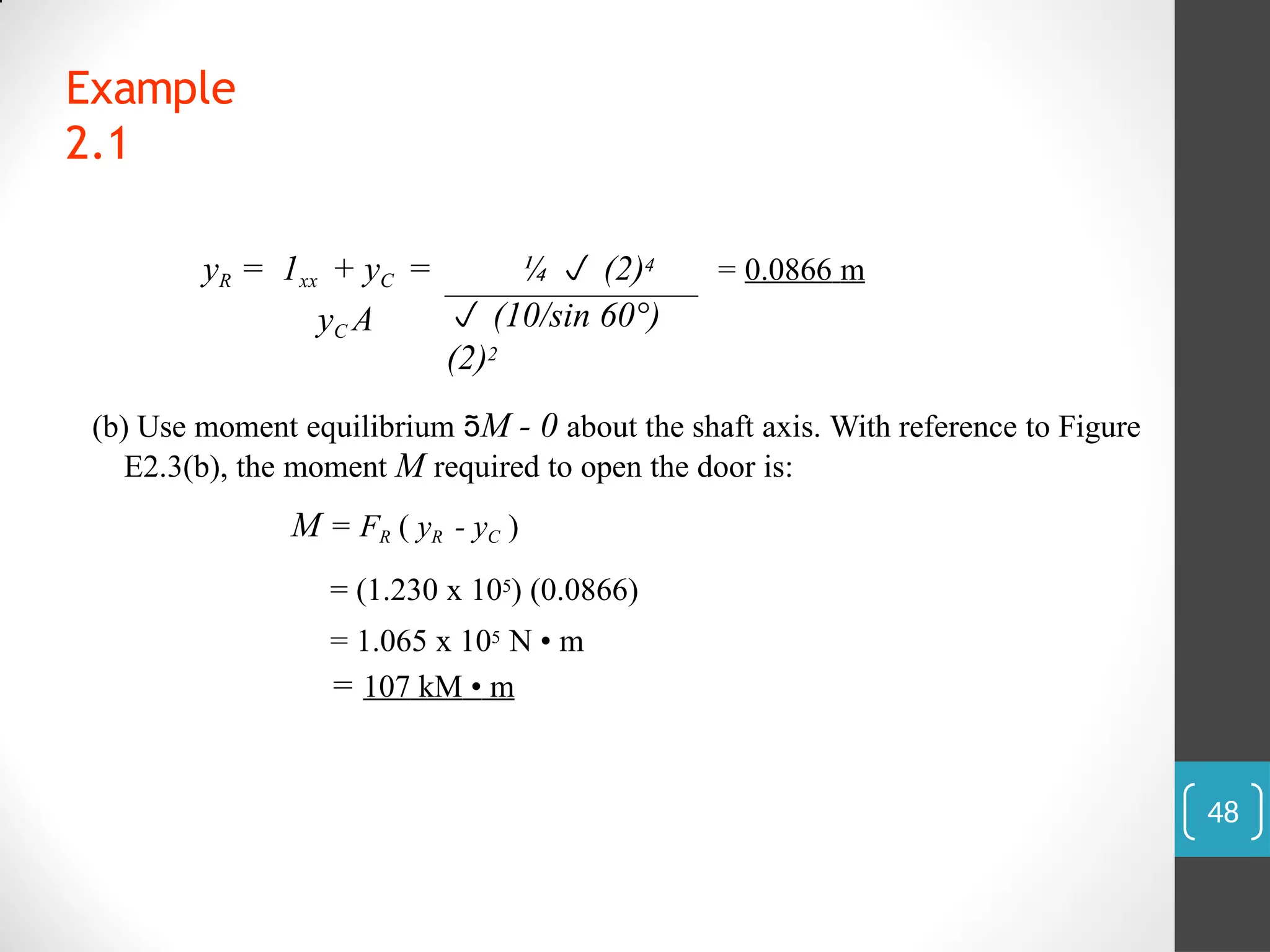
yR = 1xx + yC = ¼ R4 + yC
yC A 
yCR2
= ¼  (2)4
 (10/sin 60°)
(2)2
+ 10
sin 60°
= 11.6 m
or,
Example
2.1
47

48. Example
2.1
= 0.0866 m
yR = 1xx + yC =
yC A
¼  (2)4
 (10/sin 60°)
(2)2
(b) Use moment equilibrium M - 0 about the shaft axis. With reference to Figure
E2.3(b), the moment M required to open the door is:
M = FR ( yR - yC )
= (1.230 x 105) (0.0866)
= 1.065 x 105 N • m
= 107 kM • m
48

49. Example 2.2
Find the normal force required to
open the elliptical gate if it is hinged
at the top.
First find Ftotal, the total hydrostatic
force acting on the plate:
With (Appendix p. A-5) we get
49

50. Now calculate the slant distance between and
The slant distance to the hinge is 8m x 5m/4m = 10m, and the slant distance from the
hinge to the centroid is 2.5m. Hence,
The two moments about the hinge must add to zero:
50

51. 51

52. Example 2.3
Find magnitude and line of action of equivalent
force F.
Force balance in x and y:
52

53. The line of action of the horizontal force is
Where we just read directly off the figure.
The line of action for the vertical force can be found by summing the moments about C
(or any other point…)
(notice that we could add a constant to every x-coordinate since )
53

54. Distance from C to centroid is:
So that xcp is found to be
54

55. The complete result is summarized below:
55