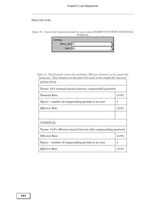
Downloaded 266 times


![Financial Analysis using Excel
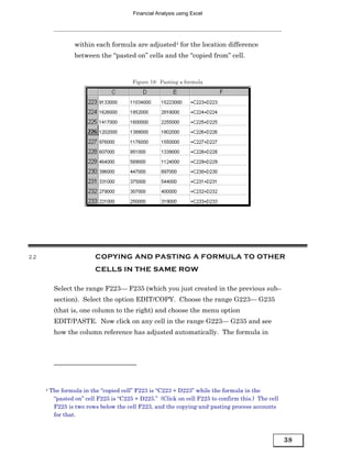
1.2.A THE “A1” VS. THE “R1C1“ STYLE OF CELL REFERENCES
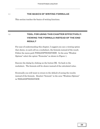
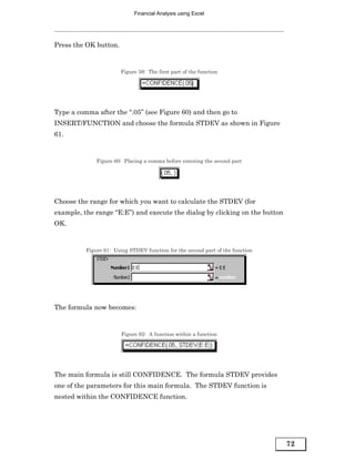
The next figure shows a simple formula. The formula is written into cell
G15. The formula multiplies the values inside cells F8 and F6.
Figure 3: A!-style cell referencing
This style of referencing is called the “A1“ style or “absolute” referencing.
The exact location of the referenced cells is written. (The cells are those
in the 6th and 8th rows of column F.) One typically works with this style.
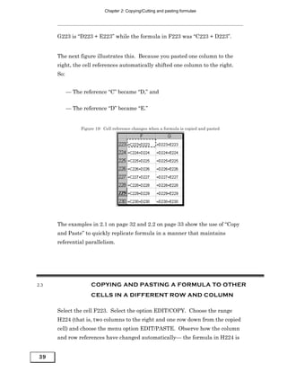
However, there is another style for referencing the cells in a formula.
This style is called the “R1C1“ style or “relative” referencing. The same
formula as in the previous figure but in R1C1 style is shown in the next
figure.
Figure 4: The same formula as in the previous figure, but in R1C1 (Offset) style cell
referencing while the previous figure showed A1 (Absolute-) style cell referencing
Does not this formula look different? This style uses relative referencing.
So, the first cell (F8) is referenced relative to its position in reference to
the cell that contains the formula (cell G15). Row 8 is 7 rows below row
15 and column F is 1 column before column G. Therefore, the cell
reference is “minus seven rows, minus 1 column” or “R[— 7]C[— 1].”
If you see a file or worksheet with such relative referencing, you can
switch all the formulas back to absolute “A1” style referencing by going to
TOOLS/OPTIONS/GENERAL and deselecting the option “R1C1 reference
style.”
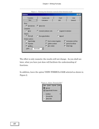
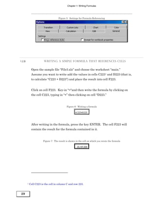
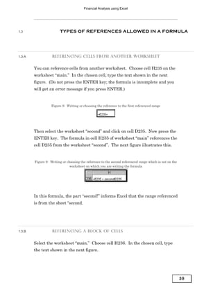
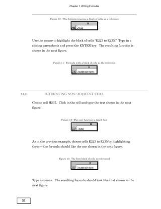
28](https://image.slidesharecdn.com/financialanalysisusingexcel-13125416666784-phpapp02-110805055501-phpapp02/85/Financial-Analysis-Using-Excel-28-320.jpg)


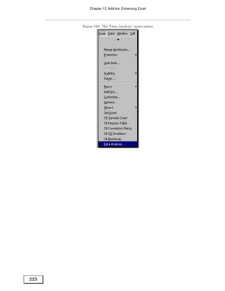


The document outlines Vijay Gupta's vision for improving office productivity and statistical software. It involves three stages: 1) Writing books to teach existing software like Excel and Word, 2) Developing tools to improve the usability of current office software, and 3) Constructing new "feedback-designed" office and statistics software from the ground up that will provide stiff competition to existing offerings like Microsoft Office. The ultimate goal is to create integrated statistical software that combines the features of programs like SPSS, Stata, and Minitab.