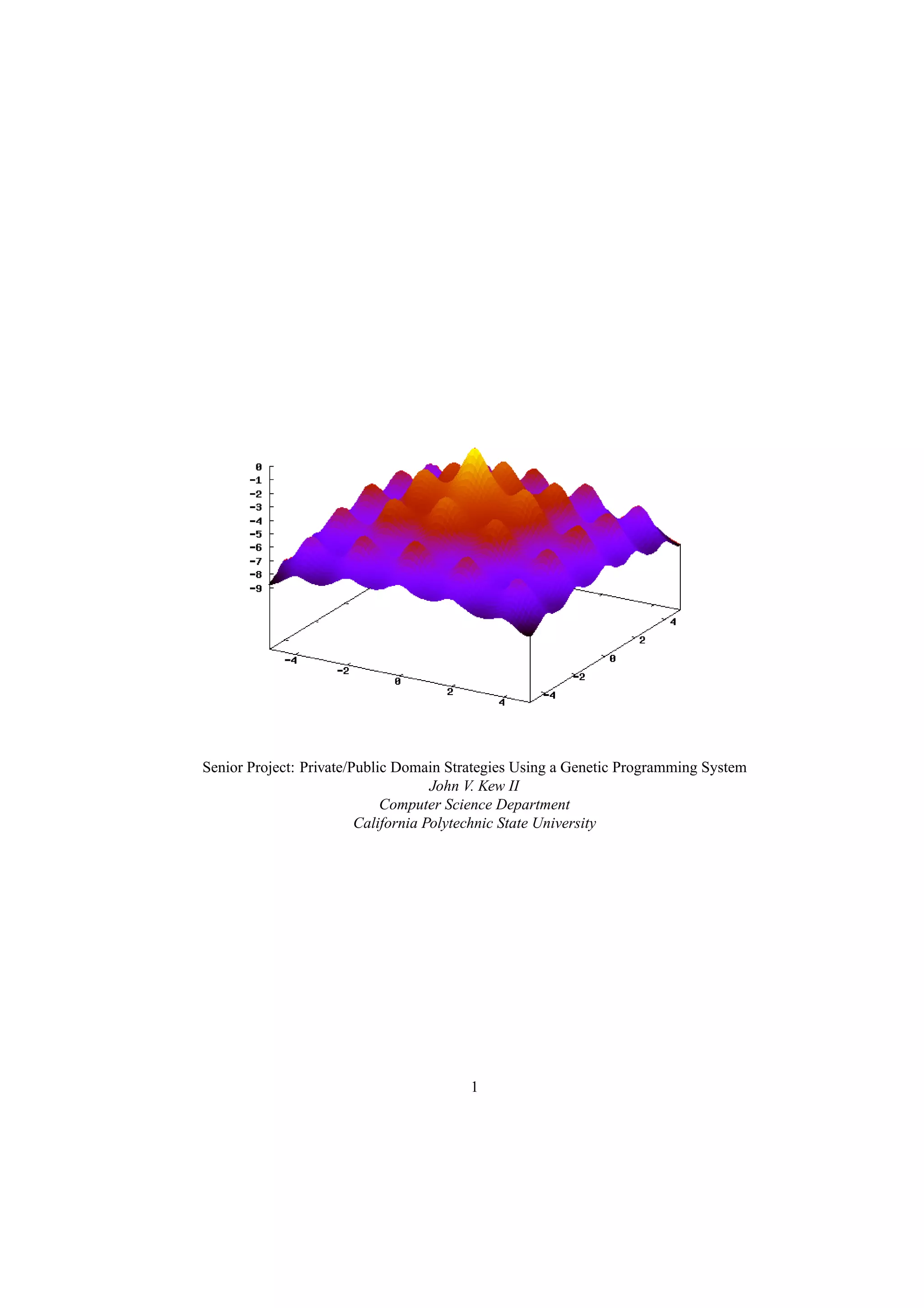
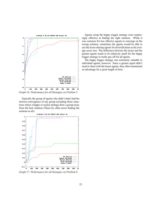
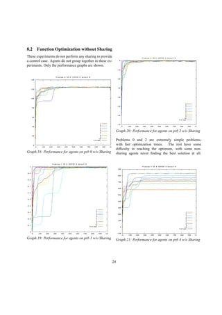
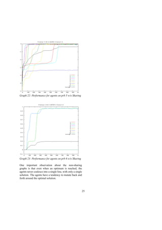
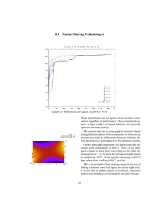
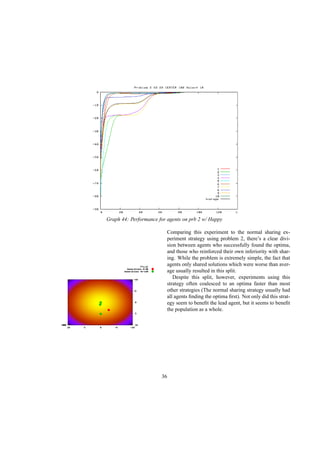
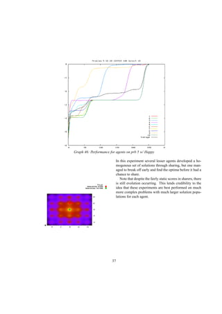
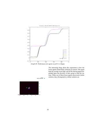
This document describes a genetic programming system that analyzes when it is better to share or hide information in a competitive environment. The system models a creative process where individuals can group solutions into private or public domains. Only solutions in the public domain can be used for crossover and mutation by all individuals. The document discusses the background of genetic programming and game theory, and how this system was designed to explore strategies around public and private domains for developing ideas. It aims to analyze the success of different sharing policies on solving problems, rather than proving effects of specific policies like patents.

![Senior Project: Private/Public Domain Strategies Using a Genetic
Programming System
John V. Kew II
Computer Science Department
California Polytechnic State University
San Luis Obispo, CA 93407
jkew@calpoly.edu
24th April 2004
“The useful arts are reproductions or new
combinations by the wit of man, of the same
natural benefactors.”
- Ralph Waldo Emerson, Nature
Abstract
The system detailed in this paper is designed for analyz-
ing when it is better to hide or share information in a com-
petitive environment. This system can be used for simple
analysis of competitive or inventive processes, with a pri-
vate domain of information and public domain of infor-
mation, and can be used as a basis for exploring more spe-
cific public/private domain problems such as copyright,
business, or psychology.
The model emulates the creative process by grouping
solutions together in one or more “domains” representing
a set of information which can be used by an agent. The
intersection of these domains is the public set of informa-
tion which can be used by any agent in the system for the
purpose of crossbreeding and mutation. Variations on this
theme include delayed dispersal of information, falsifica-
tion of information, and selective dispersal. Only selec-
tive dispersal will be explored, however the model can be
easily modified to support these variations.
Individuals have no barriers to mutation and cross
breeding within their domains but are not able to cross
breed with other domains. The children of an individual
in a domain would remain in that domain but not part of
the public domain intersection.
Originally the system was designed to find a mixed
Nash equilibrium for the sharing of information on dif-
ferent types of problems. Achieving this goal would have
required enormous computing resources and time spent in
analysis. It was more profitable to analyze different par-
ticular strategies on different classes of problems.
1 Introduction
There are numerous economic models which take advan-
tage of genetic programming. A lot of economic decision-
making can be viewed as the trek through a particular
search space of possibilities by agents seeking equilib-
rium. Rather than developing a specific set of agents
which have set strategies at each decision point, a model
using genetic programming could develop these strategies
over the course of changing economic parameters[1] and
show how private control aids in the development of ideas.
This system hopes to describe a method of exploring the
benefits of information sharing on certain innovative or
competitive processes.
It is not entirely strange to use genetic programming in
investigating strategies of private control on the
success of solutions regarding a particular problem. Spec-
ulation on the effect of various policies is rampant among
economists, psychologists, and lawyers[2]. A computing
2](https://image.slidesharecdn.com/47776ba4-6f36-46d0-a98b-69b655d611dc-150511161351-lva1-app6892/85/final-2-320.jpg)
![model which can describe these policies is not a broad
leap into wonderland. Use of genetic programming in
game theory is rampant, and this model simply adjusts
a classic payoff scheme to represent the search for a solu-
tion to a problem.
The model described is one which changes the classi-
cal GP system to simulate the propagation of ideas in an
environment where there is private control and a public
reservoir of solutions. This model could be used to evalu-
ate the relative success of lessor or greater control policies
on certain classes of problems or address aspects of policy
which might better facilitate the development of ideas.
The methods by which ideas are shared in this system
differs from existing sharing mechanisms in that specific
strategies can be assigned to each agent and modified dur-
ing the simulation. Most GP sharing methods are de-
signed to solve a specific problem quickly. This system
is designed to determine the best sharing method for a in-
dividuals or a group trying to solve a particular problem.
This model cannot prove or disprove the usefulness of
patents or copyright as the profit motive of intellectual
monopoly cannot be modeled without “profit”, and the
economic system surrounding it. It also can’t determine
specific effects of lying, managerial techniques or other
instances where information is hidden.
First described will be the classic genetic programming
model. Next, there will be a discussion of game theory as
it relates to this experiment. The Public/Private Domain
EP model will then be outlined along with issues discov-
ered during implementation followed by an address of the
assumptions made developing the model. The classes of
problems that can be represented by this model will be
looked at and lastly there will be an analysis of the exper-
iments performed with the system.
2 Background Information
One of the most difficult aspects of this system is stan-
dardizing the vocabulary used to describe it. Originally
this project was to deal directly with copyright and patent
issues. The terms used in the study of economics and in-
tellectual property must then be mapped to terms used
in genetic programming. Lack of a consistent vocabu-
lary would leave both economists and computer scientists
confused. The suggested model is also a very broad repre-
sentation of real-world intellectual property, making one
to one relationships between terms extremely difficult.
The vocabulary describing individuals and the problem
being solved will be mathematical. The vocabulary de-
scribing information dispersal and modification will be
taken from evolutionary game theory. This generaliza-
tion means that this paper could apply to any situation
where two or more groups hide information from each
other while developing an idea or process.
Game theory was the saving grace for this project. I
used Herbert Gintis’s book, Game Theory Evolving along
with Von Neumann’s Theory of Games and Economic Be-
havior extensively in this project. While my handle on
game theory is still rough the concepts explored in those
texts matched perfectly with concepts I was trying to ex-
plore with this project, but that didn’t have a standard
computer science or mathematical description. My sud-
den immersion in this field has given me the impetus to
explore more advanced issues in game theory.
2.1 Classical Evolutionary Programming
John R. Koza, a leader in genetic programming recently
wrote in the February 2003 issue of Scientific American:
Evolution is an immensely powerful cre-
ative process. From the intricate biochemistry
of individual cells to the elaborate structure
of the human unimaginable complexity. Evo-
lution achieves these fears with a few sim-
ple processes–mutation, sexual recombination
and natural selection–which it iterates for many
generations. Now computer programmers are
harnessing software versions of these same pro-
cesses to achieve machine intelligence. Called
genetic programming, this technique has de-
signed computer programs and electronic cir-
cuits that perform specified functions.
Evolutionary programming (EP) and genetic algo-
rithms (GA) utilize the same basic concept. The primary
difference between the two methods is in how the problem
is encoded. GAs typically encode problems using fixed
length tokens, where as in EP there are no limitations on
the representation[5]. Both are methods by which a solu-
tion to a problem can be sought out utilizing the processes
of natural selection and breeding.
3](https://image.slidesharecdn.com/47776ba4-6f36-46d0-a98b-69b655d611dc-150511161351-lva1-app6892/85/final-3-320.jpg)
![A set of n random solutions, called individuals are ini-
tialized and their success is tested against the problem us-
ing some sort of fitness function. The solutions which
perform better than others are copied, randomly modi-
fied, and mixed with other successful solutions for the
next “generation” of individuals. The process then restarts
until a satisfactory solution is achieved. This process can
only be performed inside of a computer, but the solutions
generated by genetic programming systems have often
been surprising and innovative.
generation
W
W
W
W
W
W
L
L
L
L
L
Figure 1: Generic genetic/evolutionary programming
Figure 1 depicts a generic genetic programming pro-
cess. Individuals, or solutions, are boxes, the solid lines
represent a basic mutation from the parent and the dotted-
dashed lines represent a cross over operation between a
successful( [W]inner ) individual in the previous genera-
tion and a newer individual. Individuals which perform
badly ( [L]oser ) do not contribute material for the next
generation of individuals.
The dependent variables in this type of system include
the number of children produced by a successful individ-
ual, degree of mutation, probability of cross over, degree
of cross over, and number of individuals in each genera-
tion.
In a classic GP system, these probabilities are deter-
mined by a normal distribution, however sometimes re-
searchers have chosen different types of distributions to
change the search performance of the system on certain
types of problems.[3] Variables such as the population
size and selection size are chosen beforehand. The prob-
lem, solution characteristics, and fitness function are also
carefully developed beforehand. An GP system is halted
at a predetermined time or when the solution meets some
criteria.
2.2 Game Theory, Private Domain and
Public Domain
This project is an analysis of the creative process between
individuals with differing information sets. The goal is
to find some sort of useful strategy between those who
share information and those who hide information[5][6].
A simple game will help describe the game theory basis
for this experiment, and give an introduction to the evolu-
tionary aspects which will be part of the full experiment.
The first game described will be a boring card game.
The game is designed to experiment with some of the is-
sues that would arise with the full version. Some of the
math behind the card game will be described and then a
repeated version of the game will be shown along with
some analysis. The repeated version of the simple game
is a very rudimentary resemblance of the full version.
The main differences between them being the strategies
available to agents, the complexity, and type of problems
solved.
A simplified version could be described as such:
Two agents draw random card from a standard deck, keep-
ing each card face down on the table. When the game
is called, the cards are flipped over and the agent with
the highest card gets three dollars. If both agents draw
the same rank, they both get one dollar. Before calling
the game, the agents each have the option of turning their
card over. If the card shown is the highest of the two cards
drawn, both agents get a dollar. The deck is shuffled and
the game starts over.
Tables 1-3 describe the normal form of the game and
their payoffs. Agent one is represented by the columns
4](https://image.slidesharecdn.com/47776ba4-6f36-46d0-a98b-69b655d611dc-150511161351-lva1-app6892/85/final-4-320.jpg)
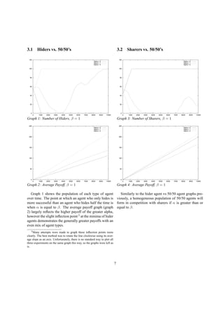
![0
50
100
150
200
250
300
350
0 1000 2000 3000 4000 5000 6000 7000 8000 9000 10000
Sharers
Hiders
Halfs
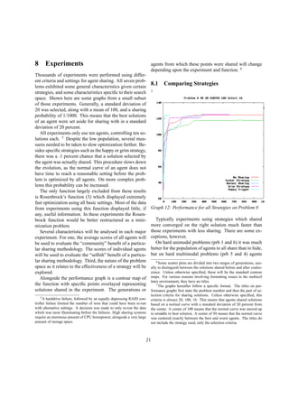
Graph 10: α = 3, β = 1
These graphs verify the conclusion that if all agents
share the same strategy, it is only beneficial for both
agents to hide if α is two times β. Since there is only one
type of each agent, only the average payoffs are graphed.
The pivot point is when alpha equals two. When α is less
than two times β, sharers prevail. The payoffs of those
agents who hide only half the time remain centered be-
tween these two extremes.
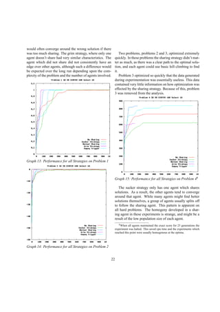
3.5 Trigger Strategies
10
15
20
25
30
35
40
45
50
55
0 2000 4000 6000 8000 10000 12000 14000 16000
Number of Defectors
Graph 11: α = 2, 50 initial defectors
The great advantage of a repeated game is the ability
to develop strategies which are dependent upon the his-
tory of the repeated game. There are two simple strate-
gies which take advantage of the repeated game, the grim
trigger strategy and the friendly trigger strategy[5].
The grim trigger strategy states that if each agent en-
counters a defector, in this case, a normally sharing agent
who decides to temporarily hide, that agent will defect, or
hide, forever. In most games this results in a population of
defectors, unless the payoff for hiding is horrifically low.
The graph above is of a strategy significantly less se-
vere than grim trigger. The friendly trigger strategy, rather
than committing an agent to defect forever, will make an
agent defect for only a set number of generations. In this
case, upon competing against a defector, the agent will de-
fect for one round only, then return to sharing. All agents
in this simulation are naturally sharers, but of the one hun-
dred agents, fifty start out defecting. Alpha and beta are
at the pivot point (α = 2 β = 1) in a homogeneous envi-
ronment where hiding and sharing are equally beneficial.
Through experimentation, it turns out that in this game,
alpha is only moderately important, defectors still lose,
but a higher alpha delays their extinction. Much more
important in this experiment is the number of rounds an
agent chooses to defect. In this simple game, a number
higher than one could almost instantly lead to a system
consisting solely of defectors.
3.6 Analysis of the Repeated Game
Repeated games offer a birds eye view of a strategic
system and the ability to develop strategies incorporating
the histories of previous games. The analysis of the full
experiment will be similar to the analysis of the simple
game. Four major questions will be answered:
1. At what point is hiding information is more worth-
while than sharing information?
2. Which homogeneous environments are the most
effective at developing solutions to problems?
3. How do trigger strategies affect the population?
4. How does the problem being solved affect the out-
come?
5. Are homogeneous or heterogeneous populations
more profitable?
9](https://image.slidesharecdn.com/47776ba4-6f36-46d0-a98b-69b655d611dc-150511161351-lva1-app6892/85/final-9-320.jpg)
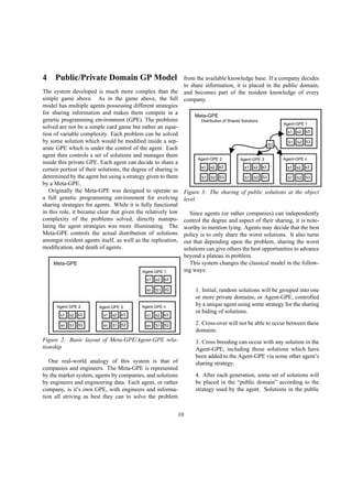
![The Meta-GPE will keep track of all agents and their
respective strategies, evolve their strategies inside a GPE,
and redistribute solutions shared to all agents. Statistics
on the average performance, curve characteristics, and
solution set size will be recorded by the Meta-GPE. The
Meta-GPE will be written in C with standard C libraries.
It will communicate with the Agent-GPE using standard
UNIX file descriptors (which could be pipes, files, or a
network connection). This allows for the distribution of
the system across multiple machines and a better way of
managing resources.
S SSSSSSSS
Likely Shared
BestWorst
figure 8: The selection of solutions to share is based on
the normal curve [8]
4.2 Agent Strategies
Of the strategies available to an agent, the trigger strate-
gies are the most important. An agent can have any mean
and standard deviation in it’s solution sharing decisions,
but because the complexity of the problems solved is rel-
atively simple, trigger strategies similar to those described
in the simple game have a more demonstrable effect upon
an experiment.
The main strategies used (besides various sharing
strategies) are the grim strategy and the happy trigger
strategy. These strategies do not technically follow their
game theory cousins. The grim strategy is not like the
grim trigger strategy. All agents using the grim strategy
are selected at the beginning of the experiment and remain
that way. The grim strategy is not "triggered". One form
of this strategy is the “Sucker” strategy, or “grim but one”
strategy where all agents hide except for a single sharing
agent.
The happy trigger strategy was also not directly taken
from existing game theory. 3
The happy trigger strategy
was a late addition to the model.
An agent using the happy trigger strategy shares only
when the average score of the agent is below the average
score of all agents. That is, if an agent is doing better
than most of the other agents, it will not share. This has
several interesting effects on problem solving, which will
be described later.
4.3 Specifics of the Agent-Problem GPE
The GPE managed by each agent is relatively simple.
Many existing GPEs are used to solve equations. The
simplicity of using mathematical functions for testing the-
ories in genetic programming are hard to escape. Each
agent in this case uses the GALib library for it’s GPE. The
GALib[15] interface is used to add and acquire shared
agents into the agents knowledge base and evolve solu-
tions to some problem. The Agent-GPE receives informa-
tion from the Meta-GPE using xml over a file descriptor
that could either be a pipe or a network connection.
4.4 Implementation Issues
The system uses a unix process for each Agent-GPE
which communicates with the Meta-GPE using xml se-
rialized c++ objects over unix file descriptors. Network
communication using SOAP and a custom object repos-
itory were researched but not pursued after the realiza-
tion that each agent would step through generations too
quickly for a distributed architecture.
Instead, the Meta-GPE starts up each agent as a sepa-
rate process and just uses file descriptors. The c++ ob-
jects containing solutions and agent commands are seri-
alized into XML using the Eternity Persistence library.
Many modifications were required to make this library
work properly using file descriptors. Additionally, seri-
alization and deserialization took a large amount of com-
puting power.
3If the happy trigger has been used in other game theory problems, it
most likely doesn’t use the name "happy." The name “sucker” was also
an invention of the author.
13](https://image.slidesharecdn.com/47776ba4-6f36-46d0-a98b-69b655d611dc-150511161351-lva1-app6892/85/final-13-320.jpg)
![These issues, and because of issues resulting from the
extreme simplicity of these problems, resulted in a config-
uration variable being added which cut into the size of the
solutions shared by each agent. Of all the solutions shared
by an agent, only a small percentage (one to ten percent)
are actually shared. This slows down the experiment to
the point where quantitative analysis of agent strategies
became useful.
Additionally, the population of agents, and the solution
population of each agent, was lowered to only ten individ-
uals. The mutation rate of each agent was also lowered.
Even with these modifications, agents in this experiment
solved problems in the test suite unexpectedly fast.
There is another issue that is apparent only in experi-
ments where there’s only a single sharing agent (sucker
strategy). In these experiments agents tend to be drawn
to the sharing agent and then get into a situation where
their score never changes before the 1000 generation is
reached.
Given the information at the time of writing, it is sup-
posed that this is due to the extremely small population
size of each agent, and the fact that agents left to share
with themselves reinforce their own homogeny.
Fortunatly the system doesn’t need to be modified to
support larger populations or more complex problems.
Unfortunately analysis requires simplicity in all these fac-
tors. Increasing the complexity of the experiments will
have to be relegated to future experiments.
5 Solution Sharing Model as Com-
pared to Existing Parallel Popula-
tion Models
There are existing methods for managing parallel popu-
lations and transferring certain members to and from the
populations. I’ll describe two here.
1. Hierarchal deterministic stepping stone
2. Overlapping populations
Hierarchal populations are a genetic programming de-
sign which uses multiple populations of individuals with
different performance characteristics. The best analogy is
that of our public education system. An individual might
start out at the lowest level, competing for survival only
among the lesser agents, and “graduate” to higher levels
depending upon their success. There are many variations
of this concept, but no standard toolset for their exploita-
tion [14].
Overlapping populations of individuals are used to
make effective use of two different environments, each
with specific mutation and breeding characteristics, by
sharing the certain individuals between their respective
populations. One environment might be good at basic hill
climbing, while the other might be good at getting out of
small ruts (using a higher mutation rate). The sharing of
individuals between these environments could potentially
reach a solution much faster (and more reliably) than a
single population alone [15].
The method described in this paper is essentially the
synthesis of these two methods. There’s been a decent
amount of research into the use of Meta-GPEs, and more
research should have been performed before reinventing
some of the methods discovered by others. 4
6 Summary of Major Assumptions
Three major assumptions have been made in this experi-
ment:
1. Functions can model a real-world problem space
2. Function optimization can model the innovative
process
3. Different types of innovative processes utilize
sharing differently
These assumptions will be described in detail in the
next sections.
4Part of the research problem was the lack of online resources at
the start. Many of the journals in which these articles appear are not
subscribed to by Cal Poly, and the two books on genetic algorithms at the
library are outdated by several years. It’s ironic that a research project
involving the use of sharing ran into problems with the accessibility of
related research.
14](https://image.slidesharecdn.com/47776ba4-6f36-46d0-a98b-69b655d611dc-150511161351-lva1-app6892/85/final-14-320.jpg)
![that information to themselves. It would have been better
for the common good if sharing was rampant, however.
A variation on this problem places the berry pickers
in a field with splotchy patches of berries. Every berry
picker is guaranteed some berries in this scenario, but not
many will be able to find the squish berries (of which there
are multiple bunches). Since squish berries grow nearby
squash berries, it is good for both the individual and the
group to share information. All pickers would desperately
love some information from their fellow picker on where
the best berries are. Since everyone wants information, it
only makes sense that agreements would be made to pro-
vide that information. While the happy trigger strategy
could develop from this scenario, squish berries come in a
multitude under this problem, so a picker would be more
likely to share information even after finding their first
batch of squish berries.
7 Set of Test Functions
The suite of test problems was organized from sev-
eral sources. Many were taken from the Matlab GEA
Toolbox[12] and others were derived from Yao, Xin and
Liu Yong’s paper, Fast Evolutionary Programming[3].
Attempts were made to develop several unimodal and
multimodal functions, along with specific search spaces
that genetic algorithms often fail to optimize.
Normally these functions are wrapped in summations
to increase their complexity. By modifying the func-
tions.h file new functions can be defined with a different
dimension. The functions tested here remained in three
dimensions so analysis could proceed more quickly.
[0] Simple Polynomial Function
This function has two optimum points at (10,5) and (-
10,-5) so agents can converge in two different directions.
This makes the problem hard for certain problems in
limited sharing environments.
Function Definition[-10:10]:
z = x2
+ xy − y2
17](https://image.slidesharecdn.com/47776ba4-6f36-46d0-a98b-69b655d611dc-150511161351-lva1-app6892/85/final-17-320.jpg)
![[1] Simple Sine Based Multimodal Function
Function Definition[-10:10]:
z =
sin(x) ∗ sin(y)
x ∗ y
[2] De Jong’s function, inverted
Simple parametric, continuous, concave, unimodal[12]
Function Definition[-10:10]:
−z = x2
+ y2
18](https://image.slidesharecdn.com/47776ba4-6f36-46d0-a98b-69b655d611dc-150511161351-lva1-app6892/85/final-18-320.jpg)
![[3] Rosenbrock’s valley, inverted
From Matlab GEA Toolbox: " Rosenbrock’s valley is
a classic optimization problem, also known as Banana
function. The global optimum is inside a long, narrow,
parabolic shaped flat valley. To find the valley is trivial,
however convergence to the global optimum is difficult
and hence this problem has been repeatedly used in
assess the performance of optimization algorithms."[12]
Agents using this problem converged too quickly,
despite it’s design. Analysis of experiments using this
problem was impossible and experiments using this
problem were disregarded.
Function Definition[-2:2]:
z = −100 ∗ (y − x2
)2
− (1 − x)2
[4] Schwefel’s Function, range adjusted
"Schwefel’s function is deceptive in that the global
minimum is geometrically distant, over the parameter
space, from the next best local minima. Therefore, the
search algorithms are potentially prone to convergence
in the wrong direction."[12][13]
Function Definition[-5:5]:
z =(x ∗ 100) ∗ sin(
2
√
x ∗ 100)+
(y ∗ 100) ∗ sin( 2
y ∗ 100)
19](https://image.slidesharecdn.com/47776ba4-6f36-46d0-a98b-69b655d611dc-150511161351-lva1-app6892/85/final-19-320.jpg)
![[5] Ackely’s Path Function, inverted.[12]
a = 10 adjusts the "flatness"
b = .2 adjusts the height of each peak
c = pi adjusts the number of peaks
Function Definition[-5:5]:
z = − (−a ∗ exp(−b ∗ 2
(x2 + y2) ∗ 1/2)−
exp((cos(c ∗ x) + cos(c ∗ y)) ∗ 1/2) + a + exp(1))
[6] Easom’s Function
The Easom function is a unimodal test function, where
the global minimum has a small area relative to the
search space. Agents outside of this area have very little
information on it’s location. The function was inverted
for maximization.[12]
Function Definition[-9:15]:
z = cos(x) ∗ cos(y) ∗ exp(−((x − Π)2
+ (y − Π)2
))
20](https://image.slidesharecdn.com/47776ba4-6f36-46d0-a98b-69b655d611dc-150511161351-lva1-app6892/85/final-20-320.jpg)


![References
[1] Harrald, Paul G. Evolutionary Algorithms and Economic Models: A View. Evolutionary Programming V, Pro-
ceedings of the Fifth Annual Conference on Evolutionary Programming, p. 4, 1996
[2] Boldrin, Michele and Levine, David. The Case Against Intellectual Monopoly, (http://levine.sscnet.ucla.edu),
Draft Chapters 1 & 2, 2003.
[3] Yao, Xin and Liu, Yong. Fast Evolutionary Programming. Evolutionary Programming V, Proceedings of the Fifth
Annual Conference on Evolutionary Programming, p. 451, 1996
[4] US Patent and Trademark Office, Website
[5] Heitkoetter, Joerg and Beasley, David. The Hitch-Hikers Guide to Evolutionary Computation,
(http://www.faqs.org/faqs/ai-faq/genetic), 2001
[6] Gintis, Herbert. Game Theory Evolving, A Problem-Centered Introduction to Modeling Strategic Interaction,
Princeton University Press, 2000
[7] Neumann, John Von, Morgenstern, Oskar. Theory of Games and Economic Behavior, Princeton University Press,
1944
[8] David Eccles School of Business. Normal Curve Image. Self Administered Statistics Test,
(http://www.business.utah.edu/masters/stattest/normal_table.htm),
[9] Levent Koçkesen, Economics W4415, Columbia University, Lecture notes,
(http://www.columbia.edu/ lk290/gameug.htm),
[10] Boost File Descriptor Stream Wrapper, (http://www.josuttis.com/cppcode),
[11] Eternity Persistence Library, (http://www.winghands.it/prodotti/eternity/overview.html),
[12] Matlab GEA Toolbox, (http://www.geatbx.com/docu/fcnfun2.html),
[13] Schwefel, H.-P. Numerical optimization of computer models, Chichester: Wiley Sons, 1981.
[14] Abrams, J. Paul. A Hierarchal Genetic Algorithm for the Travelling Salesman Problem. 95.495 Honours Project,
Carleton University, School of Computer Science, Winter, 2003
[15] Matthew’s Genetic Algorithms Library (GAlib), (http://lancet.mit.edu/ga/),
41](https://image.slidesharecdn.com/47776ba4-6f36-46d0-a98b-69b655d611dc-150511161351-lva1-app6892/85/final-41-320.jpg)

![Homogenous Population
TYPES 1.0
AGENT_ORDER {Sharer,Half,Hider}
GRIM_TRIGGER 0
FRIENDLY_TRIGGER 0
Grim Trigger -
GRIM_TRIGGER 1
FRIENDLY_TRIGGER 0
FT_DURATION 0
AGENT_ORDER {Sharer,Half,Hider}
TYPES 1.0
INITIAL_DEFECTORS int
Friendly Trigger -
FRIENDLY_TRIGGER 1
GRIM_TRIGGER 0
FT_DURATION int
AGENT_ORDER {Sharer,Half,Hider}
TYPES 1.0
INITIAL_DEFECTORS int
Card Tables:
static int samecard[2][2][2] = { { {BETA, BETA}, {BETA, BETA} },
{ {BETA, BETA}, {BETA, BETA} } };
static int greater[2][2][2] = { { {BETA, BETA}, {ZETA, ALPHA} },
{ {BETA, BETA}, {ZETA, ALPHA} } };
static int lessor[2][2][2] = { { {BETA, BETA}, {BETA, BETA} },
{ {ALPHA, ZETA}, {ALPHA, ZETA} } };
*/
#define NUMAGENTS 100 /* Number of Agents in System, int */
#define GENERATIONS 15000 /* Number of Generations, int */
#define SEXINTERVAL 100 /* Rate of Reproduction,
In Generations */
#define DEATHS 5 /* Number of Deaths per Rep. Interval */
#define MUTANTCHANCE 1 /* Percent chance of Mutation, int */
#define ALPHA 2 /* Alpha payoff rate, int - See Table*/
#define BETA 1 /* Beta payoff rate, int */
#define ZETA 0 /* Zeta payoff rate, int */
#define TYPES 1.0 /* Number of Agent Types, of type
double, used to control the nature of
the run */
43](https://image.slidesharecdn.com/47776ba4-6f36-46d0-a98b-69b655d611dc-150511161351-lva1-app6892/85/final-43-320.jpg)
![#define GRIM_TRIGGER 0 /* Grim trigger to hider state, boolean,
GRIM_TRIGGER and FRIENDLY_TRIGGER are mutually
exclusive */
#define FRIENDLY_TRIGGER 1 /* Friendly trigger to hider state */
#define FT_DURATION 1 /* Duration of the friendly trigger */
#define AGENT_ORDER {Sharer,Half,Hider} /* Agent order, used in conjuction
with "TYPES" to control nature
of run */
#define INITIAL_DEFECTORS 50 /* Initial Sharers defecting as hiders
in trigger run */
/* Cutoffs for the draw probabilities */
#define SAMECUT 3
#define GREATERCUT 27
#define TOTALPROB 53.0
void q_sort(unsigned int [][], int, int);
int main() {
int i,j,agent,agentnum,draw,value,trigger;
int decision1,decision2;
int sharers = 0,hiders = 0,halfs = 0, triggered = 0;
double average_score = 0, last_ave = 0, total_pot = 0;
/* Agent[NUMAGENTS] = [type][payoff][trigger state/count] */
unsigned int pool[NUMAGENTS][3];
/* Card Tables */
static int samecard[2][2][2] = { { {BETA, BETA}, {BETA, BETA} },
{ {BETA, BETA}, {BETA, BETA} } };
static int greater[2][2][2] = { { {BETA, BETA}, {ZETA, ALPHA} },
{ {BETA, BETA}, {ZETA, ALPHA} } };
static int lessor[2][2][2] = { { {BETA, BETA}, {BETA, BETA} },
{ {ALPHA, ZETA}, {ALPHA, ZETA} } };
/* Ordering of the agent types */
enum type AGENT_ORDER;
srand(time(0));
/* Randomly Initialize Equal Proportions of Agents */
for (i = 0; i < NUMAGENTS; i++) {
pool[i][0] = (int) (TYPES*rand()/(RAND_MAX+1.0));
pool[i][1] = 0; /* Total Value of Game to Agent */
pool[i][2] = 0; /* The finger is off the trigger */
}
44](https://image.slidesharecdn.com/47776ba4-6f36-46d0-a98b-69b655d611dc-150511161351-lva1-app6892/85/final-44-320.jpg)
![if (GRIM_TRIGGER || FRIENDLY_TRIGGER)
for (i = 0; i < INITIAL_DEFECTORS; i++)
pool[i][2] = 1;
for (i = 0; i < GENERATIONS; i++) {
halfs = 0;
sharers = 0;
hiders = 0;
triggered = 0;
for (j = 0; j < NUMAGENTS; j+=2) {
/* j is our first agent, agentnum is our second agent
- but moved to j+1 */
agentnum = j + 1 +
(int) (((double)(NUMAGENTS-1-j))*rand()/(RAND_MAX+1.0));
agent = pool[agentnum][0];
value = pool[agentnum][1];
trigger = pool[agentnum][2];
pool[agentnum][0] = pool[j+1][0];
pool[agentnum][1] = pool[j+1][1];
pool[agentnum][2] = pool[j+1][2];
pool[j+1][0] = agent;
pool[j+1][1] = value;
pool[j+1][2] = trigger;
/* Agent one decision making */
/* For the 50/50’s Decide what to do, and count the agent types */
if (pool[j][0] == Half) {
decision1 = (int) (2.0*rand()/(RAND_MAX+1.0));
halfs++;
} else {
if (pool[j][0] == Sharer) {
decision1 = 0;
sharers++;
} else if (pool[j][0] == Hider) {
decision1 = 1;
hiders++;
}
}
/* Agent two special case decision making */
if (pool[j+1][0] == Half) {
decision2 = (int) (2.0*rand()/(RAND_MAX+1.0));
halfs++;
} else {
if (pool[j+1][0] == Sharer) {
45](https://image.slidesharecdn.com/47776ba4-6f36-46d0-a98b-69b655d611dc-150511161351-lva1-app6892/85/final-45-320.jpg)
![decision2 = 0;
sharers++;
} else if (pool[j+1][0] == Hider) {
decision2 = 1;
hiders++;
}
}
/* Trigger Decisions */
if (pool[j][2] != 0) {
triggered++;
decision1 = 1;
if (pool[j][2] > 0)
pool[j][2]--; /* decrement the FT Counter */
}
if (pool[j+1][2] != 0) {
triggered++;
decision2 = 1;
if (pool[j+1][2] > 0)
pool[j+1][2]--; /* decrement the FT Counter */
}
/* Draw the cards and play the game */
draw = 1 + (int) (TOTALPROB*rand()/(RAND_MAX+1.0));
if (draw <= SAMECUT) {
pool[j][1] += samecard[decision2][decision1][1];
pool[j+1][1] += samecard[decision2][decision1][0];
} else if (draw > SAMECUT && draw <= GREATERCUT) {
pool[j][1] += greater[decision2][decision1][1];
pool[j+1][1] += greater[decision2][decision1][0];
} else {
pool[j][1] += lessor[decision2][decision1][1];
pool[j+1][1] += lessor[decision2][decision1][0];
}
total_pot = pool[j][1] + pool[j+1][1];
if (GRIM_TRIGGER) {
if (decision1 == 1)
pool[j+1][2] = -1;
if (decision2 == 1)
pool[j][2] = -1;
}
if (FRIENDLY_TRIGGER) {
if (decision1 == 1)
46](https://image.slidesharecdn.com/47776ba4-6f36-46d0-a98b-69b655d611dc-150511161351-lva1-app6892/85/final-46-320.jpg)
![pool[j+1][2] = FT_DURATION;
if (decision2 == 1)
pool[j][2] = FT_DURATION;
}
}
average_score = total_pot / NUMAGENTS;
total_pot = 0;
/* Reporting */
printf("%d %d %d %d %f %f %dn",i,sharers,hiders,halfs,average_score,
average_score - last_ave, triggered);
last_ave = average_score;
/* Reproduction of most successful agents */
if (i % SEXINTERVAL != 0)
continue;
q_sort(pool, 0, NUMAGENTS - 1);
for (j = 0; j < DEATHS; j++) {
pool[j][0] = pool[NUMAGENTS - 1 - j][0];
pool[j][1] = pool[NUMAGENTS - 1 - j][1];
pool[j][2] = pool[NUMAGENTS - 1 - j][2]; /* active defectors
replicate too */
if ((1 + (int) (100.0*rand()/(RAND_MAX+1.0))) == MUTANTCHANCE)
pool[j][0] = (int) ((TYPES)*rand()/(RAND_MAX+1.0));
}
}
return 0;
}
/* Quick sort code copied and modified from Michael Lamont’s
Knowledge Base at http://linux.wku.edu/~lamonml/kb.html and
distributed under the Open Publication License (the latest
version is presently available at http://www.opencontent.org/openpub/).
*/
void q_sort(unsigned int numbers[NUMAGENTS][3], int left, int right)
{
int pivot, l_hold, r_hold, pivot_data, more_data;
l_hold = left;
r_hold = right;
pivot = numbers[left][1];
pivot_data = numbers[left][0];
more_data = numbers[left][2];
while (left < right)
47](https://image.slidesharecdn.com/47776ba4-6f36-46d0-a98b-69b655d611dc-150511161351-lva1-app6892/85/final-47-320.jpg)
![{
while ((numbers[right][1] >= pivot) && (left < right))
right--;
if (left != right)
{
numbers[left][1] = numbers[right][1];
numbers[left][0] = numbers[right][0];
numbers[left][2] = numbers[right][2];
left++;
}
while ((numbers[left][1] <= pivot) && (left < right))
left++;
if (left != right)
{
numbers[right][0] = numbers[left][0];
numbers[right][1] = numbers[left][1];
numbers[right][2] = numbers[left][2];
right--;
}
}
numbers[left][1] = pivot;
numbers[left][0] = pivot_data;
numbers[left][2] = more_data;
pivot = left;
left = l_hold;
right = r_hold;
if (left < pivot)
q_sort(numbers, left, pivot-1);
if (right > pivot)
q_sort(numbers, pivot+1, right);
}
48](https://image.slidesharecdn.com/47776ba4-6f36-46d0-a98b-69b655d611dc-150511161351-lva1-app6892/85/final-48-320.jpg)
![Meta-GPE Source Code
#ifndef META_H
#define META_H
#include "eternity/eternity.hpp"
/* DEFAULT SETTINGS */
#define NUMAGENTS 100 /* Number of Agents in System, int */
#define GENERATIONS 100 /* Number of Generations, int */
#define SEXINTERVAL 100 /* Rate of Reproduction,
In Generations */
#define DEATHS 5 /* Number of Deaths per Rep. Interval */
#define MUTANTCHANCE 1 /* Percent chance of Mutation, int */
#define GRIM_TRIGGER 0 /* Grim trigger to hider state, boolean,
GRIM_TRIGGER and FRIENDLY_TRIGGER are
mutually exclusive */
#define FRIENDLY_TRIGGER 1 /* Friendly trigger to hider state */
#define FT_DURATION 1 /* Duration of the friendly trigger */
#define INITIAL_DEFECTORS 50 /* Initial Sharers defecting as hiders
in trigger run */
int create_agent(int fd[2],agent_control); /* send initial control file */
int step_agent(int fd[2],agent_control); /* send incremental control file */
solution_set collect_solutions(int fd[2]); /* get solutions from agent and put it in
big solution_set */
agent_stats agent_report(int fd[2]); /* get agent report, add to big stats */
void q_sort(vector< vector<double> > &numbers, int left, int right); /* sort
function */
static void sig_pipe(int);
static void sig_chld(int);
class meta_control {
public:
unsigned int dimen;
int loval;
int hival;
int prb;
unsigned int agent_popsize;
float agent_pmut;
float agent_pcross;
unsigned int initial_sdev;
unsigned int initial_mean;
unsigned int random_select;
49](https://image.slidesharecdn.com/47776ba4-6f36-46d0-a98b-69b655d611dc-150511161351-lva1-app6892/85/final-49-320.jpg)

![}
static void sig_chld(int signo) {
waitpid(-1,NULL,WNOHANG);
}
int create_agent(int fd[2], agent_control ac) {
int pid;
xml_archive out;
fd[0] = 0;
fd[1] = 0;
// create pipe
if (socketpair(AF_UNIX, SOCK_STREAM, 0, fd) < 0)
perror("Error Setting up Pipe");
if ( (pid = fork()) < 0 )
perror("Error forking");
else if (pid == 0) {
/* Advanced Programming in the Unix Enviroment pg 477 */
close(fd[0]);
if (fd[1] != STDIN_FILENO)
if (dup2(fd[1],STDIN_FILENO) != STDIN_FILENO)
perror("dup2 error in stdin redirect");
if (fd[1] != STDOUT_FILENO)
if (dup2(fd[1],STDOUT_FILENO) != STDOUT_FILENO)
perror("dup2 error in stdout redirect");
if (execl("agent", "agent", "load", "", NULL) < 0)
perror("Agent exec error");
} else {
close(fd[1]);
fd[1] = pid;
boost::fdostream outStream(fd[0]);
out.open("",archive::store, (std::iostream* ) &outStream);
ac.xml_serialize(out);
out.close();
}
return 1;
}
int step_agent(int fd[2], agent_control ac) {
xml_archive out;
boost::fdostream outStream(fd[0]);
out.open("",archive::store, (std::iostream* ) &outStream);
ac.xml_serialize(out);
outStream.clear();
out.close();
52](https://image.slidesharecdn.com/47776ba4-6f36-46d0-a98b-69b655d611dc-150511161351-lva1-app6892/85/final-52-320.jpg)
![return 1;
}
solution_set collect_solutions(int fd[2]) {
solution_set ss;
xml_archive in;
xml_archive debug;
if (kill(fd[1],SIGALRM) < 0)
perror("Unable to signal Agent");
boost::fdistream inStream(fd[0]);
in.open("",archive::load, (std::iostream* ) &inStream);
ss.xml_serialize(in);
inStream.clear();
in.close();
ss.prune();
return ss;
}
agent_stats agent_report(int fd[2]) {
agent_stats as;
xml_archive in;
boost::fdistream inStream(fd[0]);
in.open("",archive::load, (std::iostream* ) &inStream);
as.xml_serialize(in);
inStream.clear();
in.close();
// cout << "(" << as.ave_score << ")" << endl;
return as;
}
int main(int argc, char **argv) {
int i,j,agent,agentnum,draw,value,trigger;
int fd[2];
int end_count = 50;
char datafile[25];
char agentfile[25];
char status[25];
int s;
ofstream ssdat;
ofstream afile;
ofstream stats;
double ave, last_ave;
vector < vector<double> > pool;
vector <double> a;
53](https://image.slidesharecdn.com/47776ba4-6f36-46d0-a98b-69b655d611dc-150511161351-lva1-app6892/85/final-53-320.jpg)
![meta_control mc;
agent_control ac;
agent_stats as;
solution_set ss;
solution_set shared_set;
xml_archive archive;
xml_archive sharedata;
xml_archive debug;
bool cfgwrite;
bool happy_trigger;
char * cfg_file = 0;
ave = last_ave = 0;
mc.dimen = ac.dimen = 2;
mc.loval = ac.loval = -5;
mc.hival = ac.hival = 5;
mc.prb = ac.prb = 0;
mc.initial_sdev = 20;
mc.initial_mean = 50;
mc.random_select = 0;
mc.agent_popsize = ac.popsize = 100;
mc.agent_pmut = ac.pmut = .01;
mc.agent_pcross = ac.pcross = .6;
mc.select_prob = 100;
mc.popsize = NUMAGENTS;
mc.ngen = ac.ngen = GENERATIONS;
mc.sex_interval = SEXINTERVAL;
mc.deaths = DEATHS;
mc.mutant_chance = MUTANTCHANCE;
mc.grim_trigger = GRIM_TRIGGER;
mc.friendly_trigger = FRIENDLY_TRIGGER;
mc.ft_duration = FT_DURATION;
mc.initial_defectors = INITIAL_DEFECTORS;
mc.seed = ac.seed = 0;
if (argc < 2) {
cout << "Using a config file:" << endl;
cout << "meta load [file]" << endl;
cout << "Creating a default config file:" << endl;
cout << "meta write [file]" << endl;
return 0;
}
54](https://image.slidesharecdn.com/47776ba4-6f36-46d0-a98b-69b655d611dc-150511161351-lva1-app6892/85/final-54-320.jpg)
![for(int i=1; i<argc; i++) {
if(strcmp(argv[i],"load") == 0) {
cfg_file = argv[++i];
cfgwrite = false;
continue;
} else
if(strcmp(argv[i],"write") == 0) {
cfg_file = argv[++i];
cfgwrite = true;
continue;
}
}
if (cfg_file == 0) {
cout << "A config file must be specified with either ";
cout << ""load" or "write"" << endl;
return 0;
}
if (cfgwrite) {
archive.open(cfg_file, archive::store);
mc.xml_serialize(archive);
archive.close();
} else {
archive.open(cfg_file, archive::load);
mc.xml_serialize(archive);
archive.close();
}
sprintf(datafile,"data/M-%d-%d-%d.txt", mc.prb, mc.popsize, mc.ngen);
ssdat.open(datafile);
cout << "Writing Shared Solution Data to " << datafile << endl;
sprintf(datafile,"data/S-%d-%d-%d.txt", mc.prb, mc.popsize, mc.ngen);
stats.open(datafile);
cout << "Writing Statistics to " << datafile << endl;
cout << "Agent Shared Solutions are in AS-" << mc.prb;
cout << "-" << mc.popsize << "-" << mc.ngen << "-[AGENT #]" << endl;
/* Setup Default Agent Control Object */
ac.dimen = mc.dimen;
ac.loval = mc.loval;
ac.hival = mc.hival;
ac.prb = mc.prb;
ac.popsize = mc.agent_popsize;
ac.pmut = mc.agent_pmut;
55](https://image.slidesharecdn.com/47776ba4-6f36-46d0-a98b-69b655d611dc-150511161351-lva1-app6892/85/final-55-320.jpg)
![ac.pcross = mc.agent_pcross;
ac.ngen = mc.ngen;
ac.seed = mc.seed;
if (!mc.seed)
srand(time(0));
//reset pipe max to system max
// setup signal handlers
if (signal(SIGPIPE, sig_pipe) == SIG_ERR)
perror("Error Setting up SIGPIPE Handler");
if (signal(SIGCHLD, sig_chld) == SIG_ERR)
perror("Error Setting up SIGCHLD Handler");
cout << "Creating Agents" << endl;
for (i = 0; i < mc.popsize; i++) {
/* Create Agent */
a.push_back(i); /* Agent ID */
cout << "(" << a[0] << "," << i << ")";
a.push_back(0); /* Last Sucess Value of Agent */
a.push_back(0); /* The finger is off the trigger */
if (mc.random_select) {
a.push_back((int) (100.0*rand()/(RAND_MAX+1.0))); /* Position, in percent
value of normal curve */
a.push_back((int) (100.0*rand()/(RAND_MAX+1.0))); /* Standard Deviation of the
normal curve, int */
} else {
a.push_back(mc.initial_mean);
a.push_back(mc.initial_sdev);
}
a.push_back(0); /* 1st fd */
a.push_back(0); /* pid */
pool.push_back(a);
fd[0] = (int) a[5];
fd[1] = (int) a[6];
ac.id = (int) a[0];
ac.center = a[3];
ac.stddev = a[4];
ac.seed = time(0) + i;
if (!create_agent(fd,ac))
perror("Error spawning agent");
cout << ".[" << ac.id << "]";
pool[i][5] = fd[0];
pool[i][6] = fd[1];
a.clear();
}
56](https://image.slidesharecdn.com/47776ba4-6f36-46d0-a98b-69b655d611dc-150511161351-lva1-app6892/85/final-56-320.jpg)
![a.clear();
a.resize(mc.popsize, 0);
cout << endl << "Setting Initial Defectors" << endl;
if (mc.grim_trigger || mc.friendly_trigger)
for (i = 0; i < mc.initial_defectors; i++)
if (mc.grim_trigger)
pool[i][2] = -1; /* Agent will defect permenantly */
else
pool[i][2] = mc.ft_duration;
if (mc.ft_duration == -2) /* Happy Trigger is set */
happy_trigger = true;
cout << "Starting Evolution" << endl;
for (i = 0; i < mc.ngen; i++) {
cout << "GENERATION " << i << " [";
stats << i << " ";
/* Test Agents */
/* Distribution of Solutions */
//ac.shared = shared_set;
for (j = 0; j < mc.popsize; j++) {
fd[0] = (int) pool[j][5];
fd[1] = (int) pool[j][6];
ac.id = (int) pool[j][0];
ac.center = pool[j][3];
ac.stddev = pool[j][4];
if (!step_agent(fd,ac))
perror("Error stepping agent");
cout << ".";
cout.flush();
}
/* Set Triggers */
/* Reporting */
cout << "]-R-[";
cout.flush();
shared_set.clear();
last_ave = ave;
ave = 0;
for (j = 0; j < mc.popsize; j++) {
ss.clear();
fd[0] = (int) pool[j][5];
fd[1] = (int) pool[j][6];
ac.id = (int) pool[j][0];
ac.center = pool[j][3];
57](https://image.slidesharecdn.com/47776ba4-6f36-46d0-a98b-69b655d611dc-150511161351-lva1-app6892/85/final-57-320.jpg)
![ac.stddev = pool[j][4];
as = agent_report(fd);
ss = collect_solutions(fd);
/* Do something with the statistics */
/* get a listing of agent scores ordered by agent id */
pool[j][1] = a[((int) pool[j][0])] = as.ave_score;
ave += as.ave_score;
sprintf(agentfile,"data/AS-%d-%d-%d-%d.txt", mc.prb, mc.popsize, mc.ngen,
(int) ac.id);
afile.open(agentfile, ofstream::out | ofstream::app);
afile << "# Generation " << i << endl;
ss.write(afile);
afile.close();
/* add in solution set */
/* p/10000 only add solutions if not triggered */
if (pool[j][2] == 0 || (happy_trigger && i > 0 && as.ave_score <= last_ave) ){
shared_set.add_some_solutions(mc.select_prob,ss);
} else
if (mc.friendly_trigger)
pool[j][2]--; /* Decrement the friendly trigger */
cout << ".";
cout.flush();
}
ssdat << "# Generation " << i << endl;
shared_set.write(ssdat);
ave = ave / mc.popsize;
for (j = 0; j < mc.popsize; j++)
stats << a[j] << " ";
stats << ave << " " << shared_set.size() << endl;
cout << "][" << ave << "]-S-[" << shared_set.size() << "]";
/* The Shared Solutions are about the only thing that is easily shared
off of one file... this can be a very large file */
sharedata.open("current_shared_solutions.xml", archive::store);
shared_set.xml_serialize(sharedata);
sharedata.close();
/* Writing Shared Solutions to Data File*/
//ssdat << i << " " << shared_set.size() << " ";
ssdat.flush();
//ssdat << endl;
/* Notify agents that the solutions are available */
for (j = 0; j < mc.popsize; j++)
58](https://image.slidesharecdn.com/47776ba4-6f36-46d0-a98b-69b655d611dc-150511161351-lva1-app6892/85/final-58-320.jpg)
![if (kill((int)pool[j][6],SIGALRM) < 0)
perror("Unable to signal Agent");
/* Reproduction of most successful agents, Death, and Mutation */
cout << "-S-";
if (i % mc.sex_interval != 0)
continue;
q_sort(pool, 0, mc.popsize - 1);
if (pool[0][1] == pool[mc.popsize - 1][1]) {
if (!end_count) {
cout << endl << "Worst Agent Score Equals Best Agent Score" << endl;
cout << "Killing agents:";
for (j = 0; j < mc.popsize; j++) {
if (kill((int)pool[j][6],SIGKILL) < 0)
perror("Unable to signal Agent");
cout << ".";
}
cout << endl;
break;
} else
end_count--;
} else if (end_count != 50)
end_count = 50;
cout << "M-";
for (j = 0; j < mc.deaths; j++) {
// Mark Agent Death
//sprintf(agentfile,"data/AS-%d-%d-%d-%d.txt", mc.prb, mc.popsize, mc.ngen, j);
//afile.open(agentfile, ofstream::out | ofstream::app);
//afile << "# AGENT DEATH" << i << endl;
//afile.close();
cout << "[" << pool[j][0] << "," << pool[mc.popsize - 1 - j][0] << "]";
cout << "[" << pool[j][1] << "," << pool[mc.popsize - 1 - j][1] << "]";
//pool[j][0] = i + pool[j][0]/1000; /* New Agent ID = gen.(deadid/1000) */
pool[j][1] = pool[mc.popsize - 1 - j][1]; /* Score */
//pool[j][2] = pool[mc.popsize - 1 - j][2]; /* active defectors */
pool[j][3] = pool[mc.popsize - 1 - j][3]; /* Curve Position */
pool[j][4] = pool[mc.popsize - 1 - j][4]; /* Std Dev*/
/* replicate too */
/* Insert Mutation Code Here */
if (((int) (100.0*rand()/RAND_MAX+1.0)+1) <= mc.mutant_chance) {
draw = 0;
if (pool[j][3] < 100 & pool[j][3] > 0)
draw = ((int) (3.0*rand()/RAND_MAX+1)) - 2;
59](https://image.slidesharecdn.com/47776ba4-6f36-46d0-a98b-69b655d611dc-150511161351-lva1-app6892/85/final-59-320.jpg)
![pool[j][3] += draw;
cout << "[" << draw << ",";
draw = 0;
if (pool[j][4] < 100 & pool[j][4] > 0)
draw = ((int) (3.0*rand()/RAND_MAX+1)) - 2;
pool[j][4] += draw;
cout << draw << "]";
}
}
cout << "DONE" << endl;
cout.flush();
}
cout << endl;
ssdat.close();
stats.close();
return 0;
}
/* Quick sort code copied and modified from Michael Lamont’s
Knowledge Base at http://linux.wku.edu/~lamonml/kb.html and
distributed under the Open Publication License (the latest
version is presently available at http://www.opencontent.org/openpub/).
*/
void q_sort(vector< vector<double> > &numbers, int left, int right)
{
double pivot;
int l_hold, r_hold, i;
double data[7];
l_hold = left;
r_hold = right;
pivot = numbers[left][1];
for (i=0; i < 7; i++)
data[i] = numbers[left][i];
while (left < right)
{
while ((numbers[right][1] >= pivot) && (left < right))
right--;
if (left != right)
{
for (i=0; i < 7; i++)
numbers[left][i] = numbers[right][i];
left++;
}
60](https://image.slidesharecdn.com/47776ba4-6f36-46d0-a98b-69b655d611dc-150511161351-lva1-app6892/85/final-60-320.jpg)
![while ((numbers[left][1] <= pivot) && (left < right))
left++;
if (left != right)
{
for (i=0; i < 7; i++)
numbers[right][i] = numbers[left][i];
right--;
}
}
for (i=0; i < 7; i++)
numbers[left][i] = data[i];
pivot = left;
left = l_hold;
right = r_hold;
if (left < pivot)
q_sort(numbers, left, (int) pivot-1);
if (right > pivot)
q_sort(numbers, (int) pivot+1, right);
}
#endif
61](https://image.slidesharecdn.com/47776ba4-6f36-46d0-a98b-69b655d611dc-150511161351-lva1-app6892/85/final-61-320.jpg)

![unsigned int popsize = 30;
unsigned int ngen = 100;
float pmut = 0.01;
float pcross = 0.6;
float center = 50;
float stddev = 30;
bool cfgwrite = false;
meta_ready = false;
agent_control ac;
solution_set ss;
agent_stats as;
xml_archive archive;
xml_archive out;
xml_archive dout;
xml_archive stdout;
xml_archive stdout2;
GABin2DecPhenotype map;
GAPopulation population;
boost::fdostream outStream(STDOUT_FILENO);
if (signal(SIGABRT, sig_abrt) == SIG_ERR)
perror("Error Setting up SIGABRT Handler");
if (signal(SIGALRM, sig_alrm) == SIG_ERR)
perror("Error Setting up SIGALRM Handler");
if (argc < 2) {
cout << "Loading a config file:" << endl;
cout << "agent load [file] [state_file [file]]" << endl << endl;
cout << "Creating a config file:" << endl;
cout << "agent write [file] seed [seed] dimension [dimen] low [loval]";
cout << "high [hival] popsize [popsize] ngen [ngen] pmut [pmut]";
cout << "pcross [pcross] agent_id [id] state_file [filename] problem [prb #]";
cout << endl;
return 0;
}
for(int i=1; i<argc; i++) {
if(strcmp(argv[i],"seed") == 0) {
seed = atoi(argv[++i]);
continue;
} else
if(strcmp(argv[i],"dimension") == 0) {
dimen = atoi(argv[++i]);
continue;
66](https://image.slidesharecdn.com/47776ba4-6f36-46d0-a98b-69b655d611dc-150511161351-lva1-app6892/85/final-66-320.jpg)
![} else
if(strcmp(argv[i],"high") == 0) {
hival = atoi(argv[++i]);
continue;
} else
if(strcmp(argv[i],"low") == 0) {
loval = atoi(argv[++i]);
continue;
} else
if(strcmp(argv[i],"popsize") == 0) {
popsize = atoi(argv[++i]);
continue;
} else
if(strcmp(argv[i],"ngen") == 0) {
ngen = atoi(argv[++i]);
continue;
} else
if(strcmp(argv[i],"pmut") == 0) {
pmut = atof(argv[++i]);
continue;
} else
if(strcmp(argv[i],"pcross") == 0) {
pcross = atof(argv[++i]);
continue;
} else
if(strcmp(argv[i],"agent_id") == 0) {
id = atoi(argv[++i]);
continue;
} else
if(strcmp(argv[i],"state_file") == 0) {
state_file = argv[++i];
continue;
} else
if(strcmp(argv[i],"problem") == 0) {
prb = atoi(argv[++i]);
continue;
} else
if(strcmp(argv[i],"load") == 0) {
cfg_file = argv[++i];
cfgwrite = false;
continue;
} else
if(strcmp(argv[i],"write") == 0) {
cfg_file = argv[++i];
cfgwrite = true;
continue;
67](https://image.slidesharecdn.com/47776ba4-6f36-46d0-a98b-69b655d611dc-150511161351-lva1-app6892/85/final-67-320.jpg)
![}
}
if (cfg_file == 0) {
cout << "A config file must be specified with either ";
cout << ""load" or "store"" << endl;
return 0;
}
if (cfgwrite) {
ac.dimen = dimen;
ac.loval = loval;
ac.hival = hival;
ac.id = id;
ac.prb = prb;
ac.popsize = popsize;
ac.ngen = ngen;
ac.pmut = pmut;
ac.pcross = pcross;
ac.center = center;
ac.stddev = stddev;
archive.open(cfg_file, archive::store);
ac.xml_serialize(archive);
archive.close();
return 0;
} else {
if (cfg_file[0] == ’0’) {
debug << "stdin load" << endl;
out.open("", archive::load);
debug << "stdin serialize" << endl;
ac.xml_serialize(out);
debug << "stdin close" << endl;
out.close();
} else {
debug << "file load" << endl;
archive.open(cfg_file, archive::load);
ac.xml_serialize(archive);
archive.close();
}
}
if (!ac.seed)
srand(time(0));
else
srand(ac.seed);
68](https://image.slidesharecdn.com/47776ba4-6f36-46d0-a98b-69b655d611dc-150511161351-lva1-app6892/85/final-68-320.jpg)
![for (int i = 0; i < ac.dimen; i++)
map.add(16, lorange[ac.prb], hirange[ac.prb]);
GABin2DecGenome genome(map, functions[ac.prb]);
GASimpleGA ga(genome);
GASigmaTruncationScaling scaling;
ga.populationSize(ac.popsize);
ga.nGenerations(ac.ngen);
ga.pMutation(ac.pmut);
ga.pCrossover(ac.pcross);
ga.scaling(scaling);
ga.scoreFilename();
ga.initialize(time(0));
for (int i = 0; i < ac.ngen; i++) {
// Reread Control File if expecting it from stdin
if (cfg_file[0] == ’0’) {
out.open("", archive::load);
ac.xml_serialize(out);
out.close();
}
ga.step();
/* Resize back to Normal Population Size */
ga.populationSize(ac.popsize);
population = ga.population();
ss.clear();
ss.isSelective(true);
as.setStatistics(population, ga.statistics());
ss.setSelectionCriteria(adjMean95(as.max_score, as.min_score,
as.ave_score, as.std_dev, ac.center),
adjStddev95(as.max_score, as.min_score,
as.ave_score, as.std_dev, ac.stddev));
ss.setSolutions(population);
stdout.open("", archive::store);
as.xml_serialize(stdout);
stdout.close();
69](https://image.slidesharecdn.com/47776ba4-6f36-46d0-a98b-69b655d611dc-150511161351-lva1-app6892/85/final-69-320.jpg)
![/* Synchronize with Meta-GPE */
while (!meta_ready || cfg_file[0] != ’0’)
sleep(1);
meta_ready = false;
stdout2.open("", archive::store);
ss.xml_serialize(stdout2);
stdout2.close();
//sleep(5); DELETE ME
dout.open("agent.debug",archive::store);
ss.xml_serialize(dout);
dout.close();
cout.flush();
ss.isSelective(false);
/* Synchronize with Meta-GPE */
while (!meta_ready || cfg_file[0] != ’0’)
sleep(1);
meta_ready = false;
ss.clear();
archive.open("current_shared_solutions.xml", archive::load);
ss.xml_serialize(archive);
archive.close();
/* Add Shared Genomes to the population */
GAPopulation *pop = ga.population().clone();
for (int j = 0; j < ss.size(); j++) {
pop->add((ss.get_solution(j).getGenome()).clone());
}
pop->statistics(gaTrue);
pop->scale();
pop->sort(gaTrue);
ga.population(*pop);
}
return 0;
}
70](https://image.slidesharecdn.com/47776ba4-6f36-46d0-a98b-69b655d611dc-150511161351-lva1-app6892/85/final-70-320.jpg)
![float center;
float stddev;
public:
solution() { dimension = 0; score = 0; hival=0; loval=0;}
solution(GABin2DecGenome &g) { setSolution(g); }
float get_phen(int i) { return ((phenotype) phen[i]).getPhen();}
GABin2DecGenome getGenome();
void setSolution(GABin2DecGenome &g);
void add_phen(phenotype &p) {phen.push_back(p); dimension++;}
void add_phen(int i, float d) { add_phen(*(new phenotype(i,d)));}
void add_phen(int i, float d, float l, float h) {add_phen(i,d); loval = l;
hival = h;}
void prune(void);
void write(ostream &out);
void xml_serialize( xml_archive &xml);
};
class solution_set {
private:
vector<solution> solutions;
bool beSelective;
float mean; // Mean of dist
float stddev;
float probability(float x, float m, float s);
float probability(float x) { return probability(x, mean, stddev); }
bool isIncluded(float x);
public:
solution_set() { mean = 0; stddev = 0; beSelective = false;}
~solution_set() { solutions.clear(); }
void add_solution(solution &s) { solutions.push_back(s); }
void add_solution(GABin2DecGenome &g);
solution& get_solution(int i) { if (i < solutions.size()) return solutions[i]; }
int size() { return solutions.size(); }
void add_some_solutions(int p, solution_set ss) {
for (int i=0; i < ss.size(); i++)
if (((int) (10000.0*rand()/RAND_MAX+1.0) + 1) <= p)
add_solution((solution&)ss.get_solution(i));
}
void add_solutions(solution_set ss){
for (int i=0; i < ss.size(); i++)
add_solution((solution&)ss.get_solution(i)); }
void clear() { solutions.clear(); }
void prune(void);
void setSolutions(const GAPopulation &p);
72](https://image.slidesharecdn.com/47776ba4-6f36-46d0-a98b-69b655d611dc-150511161351-lva1-app6892/85/final-72-320.jpg)

![xml.write("datum",datum);
}
}
GABin2DecGenome solution::getGenome() {
GABin2DecPhenotype map;
GAReportErrors(gaFalse);
dimension = 2;
for (int i = 0; i < dimension; i++)
map.add(BITS, loval, hival);
GABin2DecGenome genome(map);
genome.initialize();
for (int d = dimension; d > 0; d--)
genome.phenotype((d-1), phen[(d-1)].getPhen());
genome.score(score);
return genome;
}
void solution::setSolution(GABin2DecGenome &g) {
int d;
hival = ((GABin2DecPhenotype) g.phenotypes()).max(0);
loval = ((GABin2DecPhenotype) g.phenotypes()).min(0);
phen.clear();
dimension = 0;
score = 0;
for (d = 0; d < g.nPhenotypes(); d++)
add_phen(d, g.phenotype(d));
dimension = d;
score = g.score();
}
void solution::write(ostream &out) {
vector<phenotype>::iterator pn;
//out << dimension << " ";
for (pn = phen.begin(); pn != phen.end(); pn++)
pn->write(out);
out << endl;
}
void solution::prune() {
vector<phenotype>::iterator pn;
pn = phen.begin();
pn += dimension;
if (pn < phen.end())
phen.erase(pn,phen.end());
}
74](https://image.slidesharecdn.com/47776ba4-6f36-46d0-a98b-69b655d611dc-150511161351-lva1-app6892/85/final-74-320.jpg)


![Functions Source Code
#ifndef FUNCTIONS_H
#define FUNCTIONS_H
#include <math.h>
#include <ga/ga.h>
#define PI (3.1415926535897932384626433832795028841971693993751f)
/* y=a^2 + ab - b^2
This function defines the search space of the problem, and given a
solution, returns it’s value y=a^2 + ab - b^2
It requires 2 phenotypes per genome.
f(x,y) = x**2 + x*y - y**2 # 0 GNUPLOT fn
set xrange [-10:10] # 0 GNUPLOT xrange
set yrange [-10:10] # 0 GNUPLOT yrange
set title "fn0 Polynomial" # 0 GNUPLOT title
*/
float polynomial(GAGenome &c) {
GABin2DecGenome &genome = (GABin2DecGenome &)c;
float y;
y = genome.phenotype(0) * genome.phenotype(0);
y += genome.phenotype(0) * genome.phenotype(1);
y -= genome.phenotype(1) * genome.phenotype(1);
return y;
}
/* y=(sin(a)*sin(b))/(a*b)
Range -10 to 10 for a and b
f(x,y) = (sin(x)*sin(y))/(x*y) # 1 GNUPLOT fn
set xrange [-10:10] # 1 GNUPLOT xrange
set yrange [-10:10] # 1 GNUPLOT yrange
set title "fn1 Basic MultiModalSine" # 1 GNUPLOT title
*/
float MultiModalSineBased(GAGenome &c) {
GABin2DecGenome & genome = (GABin2DecGenome &)c;
float y;
float a = genome.phenotype(0);
float b = genome.phenotype(1);
y = (sin(a)*sin(b))/(a*b);
return y;
}
81](https://image.slidesharecdn.com/47776ba4-6f36-46d0-a98b-69b655d611dc-150511161351-lva1-app6892/85/final-81-320.jpg)
![/* -y=a^2 + b^2
De Jong’s function, inverted
Simple parametric, continous, concave, unimodal
(The original was convex, but since we are maximizing...)
Maxima at 0,0
Range -10, 10
Matlab GEA Toolbox
http://www.geatbx.com/docu/fcnfun1.html
f(x,y) = -(x**2 + y**2) # 2 GNUPLOT fn
set xrange [-10:10] # 2 GNUPLOT xrange
set yrange [-10:10] # 2 GNUPLOT yrange
set title "fn2 DeJong" # 2 GNUPLOT title
*/
float DeJong(GAGenome &c) {
GABin2DecGenome & genome = (GABin2DecGenome &)c;
float y;
float a = genome.phenotype(0);
float b = genome.phenotype(1);
y = a*a + b*b;
return -y;
}
/* y=-100*(y-x^2)^2-(1-x)^2
Rosenbrock’s valley, inverted
f2(x)=sum(100·(x(i+1)-x(i)^2)^2+(1-x(i))^2), i=1:n-1
Range: -2:2
" Rosenbrock’s valley is a classic optimization problem, also known as
Banana function. The global optimum is inside a long, narrow, parabolic
shaped flat valley. To find the valley is trivial, however convergence
to the global optimum is difficult and hence this problem has been
repeatedly used in assess the performance of optimization algorithms."
Matlab GEA Toolbox
http://www.geatbx.com/docu/fcnfun2.html
f(x,y) = -100*(y-x*x)*(y-x*x) - (1-x)*(1-x) # 3 GNUPLOT fn
set xrange [-2:2] # 3 GNUPLOT xrange
set yrange [-2:2] # 3 GNUPLOT yrange
set title "fn3 Rosenbrock" # 3 GNUPLOT title
*/
float Rosenbrock(GAGenome &c) {
GABin2DecGenome & genome = (GABin2DecGenome &)c;
82](https://image.slidesharecdn.com/47776ba4-6f36-46d0-a98b-69b655d611dc-150511161351-lva1-app6892/85/final-82-320.jpg)
![float y;
float a = genome.phenotype(0);
float b = genome.phenotype(1);
y = -100*(b-a*a)*(b-a*a) - (1-a)*(1-a);
return y;
}
/* y=(a*100)*sin(sqrt(abs(a*100)))+(b*100)*sin(sqrt(abs(b*100)))
Schwefel’s Function, range adjusted
Original: f7(x)=sum(-x(i)·sin(sqrt(abs(x(i))))), i=1:n; -500 to 500
New Range: -5:5
"Schwefel’s function is deceptive in that the global minimum is geometrically
distant, over the parameter space, from the next best local minima. Therefore,
the search algorithms are potentially prone to convergence in the wrong
direction."
Matlab GEA Toolbox
http://www.geatbx.com/docu/fcnfun7.html
Additional Resources:
Schwefel, H.-P.: Numerical optimization of computer models. Chichester:
Wiley & Sons, 1981.
f(x,y) = (x*100)*sin(sqrt(abs(x*100)))+(y*100)*sin(sqrt(abs(y*100))) # 4 GNUPLOT fn
set xrange [-5:5] # 4 GNUPLOT xrange
set yrange [-5:5] # 4 GNUPLOT yrange
set title "fn4 Schwefel" # 4 GNUPLOT title
*/
float Schwefel(GAGenome &c) {
GABin2DecGenome & genome = (GABin2DecGenome &)c;
float y;
float a = genome.phenotype(0);
float b = genome.phenotype(1);
y=(a*100)*sin(sqrt(abs(a*100)))+(b*100)*sin(sqrt(abs(b*100)));
return y;
}
/* z=-(-a*exp(-b*sqrt((x*x+y*y)*1/2))-exp((cos(c*x)+cos(c*y))*1/2)+a+exp(1))
Ackely’s Path Function, range adjusted, inverted
Original: f10(x)=-a·exp(-b·sqrt(1/n·sum(x(i)^2)))-exp(1/n·sum(cos(c·x(i))))+a+exp(1);
83](https://image.slidesharecdn.com/47776ba4-6f36-46d0-a98b-69b655d611dc-150511161351-lva1-app6892/85/final-83-320.jpg)
![a=20; b=0.2; c=2·pi; i=1:n;
-32.768<=x(i)<=32.768.
Implemented:
a=10; b=.2; c=pi
Range -5:5
a adjusts the "flatness"
b adjusts the height of each peak
c adjusts the number of peaks
Matlab GEA Toolbox
http://www.geatbx.com/docu/fcnfun10.html
a = 10 # 5 GNUPLOT vr
b = .2 # 5 GNUPLOT vr
c = pi # 5 GNUPLOT vr
f(x,y) = -(-a*exp(-b*sqrt((x*x+y*y)*1/2))-exp((cos(c*x)+cos(c*y))*1/2)+a+exp(1.0)) # 5 G
set xrange [-5:5] # 5 GNUPLOT xrange
set yrange [-5:5] # 5 GNUPLOT yrang
set title "fn5 Ackely" # 5 GNUPLOT title
*/
float Ackely(GAGenome &g) {
GABin2DecGenome & genome = (GABin2DecGenome &)g;
float z;
float x = genome.phenotype(0);
float y = genome.phenotype(1);
float a = 10;
float b = .2;
float c = PI;
z=-(-a*exp(-b*sqrt((x*x+y*y)*1/2))-exp((cos(c*x)+cos(c*y))*1/2)+a+exp(1.0));
return z;
}
/* Easoms function
The Easom function is a unimodal test function, where the
global minimum has a small area relative to the search
space. The function was inverted for minimization.
Original function definition:
fEaso(x1,x2)=-cos(x1)·cos(x2)·exp(-((x1-pi)^2+(x2-pi)^2));
-100<=x(i)<=100, i=1:2.
Implemented:
z = cos(x)*cos(y)*exp(-((x-PI)**2+(y-PI)**2))
84](https://image.slidesharecdn.com/47776ba4-6f36-46d0-a98b-69b655d611dc-150511161351-lva1-app6892/85/final-84-320.jpg)
![range: -9:15
global minimum
f(x1,x2)=-1; (x1,x2)=(pi,pi).
f(x,y) = cos(x)*cos(y)*exp(-((x-pi)*(x-pi)+(y-pi)*(y-pi))) # 6 GNUPLOT fn
set xrange [-9:15] # 6 GNUPLOT xrange
set yrange [-9:15] # 6 GNUPLOT yrange
set title "fn6 Easom" # 6 GNUPLOT title
*/
float Easoms(GAGenome &g) {
GABin2DecGenome & genome = (GABin2DecGenome &)g;
float z;
float x = genome.phenotype(0);
float y = genome.phenotype(1);
z = cos(x)*cos(y)*exp(-((x-PI)*(x-PI)+(y-PI)*(y-PI)));
return z;
}
float (*functions[7])(GAGenome &) = {polynomial,MultiModalSineBased,
DeJong,Rosenbrock,Schwefel,Ackely,Easoms};
int hirange[7] = {10,10,10,2,5,5,15};
int lorange[7] = {-10,-10,-10,-2,-5,-5,-9};
#endif
85](https://image.slidesharecdn.com/47776ba4-6f36-46d0-a98b-69b655d611dc-150511161351-lva1-app6892/85/final-85-320.jpg)