1. Abstract—The purpose of this lab is to find material properties
for two specimens using compressive testing. Students willanalyze
and compare the material properties found by quasi-static and
dynamic loading. The data that was taken on the UTS for the
quasi-staticloading was provided online by the professor. Students
used the Split-Hopkinson Pressure Bar to record data for the
dynamic loading. Students then found the material properties
from this raw data. This was done by using variations of stress and
strain equations as well as using knowledge of wave propagation
theory as it applied to the Split-Hopkinson Pressure Bar. It was
found that the Young’s Modulus and yield strength were higher
for both specimens in dynamic loading compared to quasi-static
loading.
Index Terms—Oscilloscope, Quasi-static loading, Split-
Hopkinson Bar Pressure, Wave Propagation Theory.
I. INTRODUCTION
The purpose of this final lab project is to determine the
material properties that a certain material displays under two
different loading methods, dynamic and quasi-static. If the
strain rate is found to be > 0.01 𝑠−1
, the loading is said to be
dynamic. If strain rate is found to be < 0.01 𝑠−1
, the loading is
said to be quasi-static.The strain rate a material is subjected to
is a large factor in determining its material properties.
To obtain data for the material properties using quasi-static
loading, the Instron 5967 Universal Testing Machine (UTS) is
used. The specimens are subjected to compressive loading
where the UTS will determine the strain for the specific loading.
Students did not physically use the UTS but data was taken and
provided by the professor for analysis and comparisons to the
material properties found by dynamic loading.
In order to obtain data for the material properties using
dynamic loading, students used the Split-Hopkinson Pressure
Bar. Voltage signals will be measured via an oscilloscope.
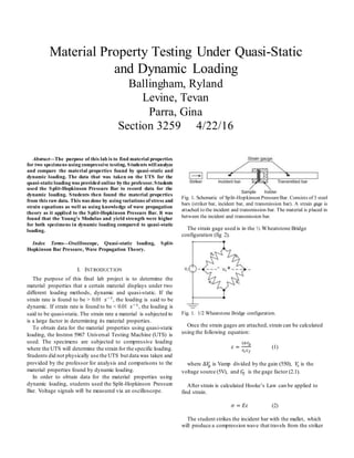
Fig. 1. Schematic of Split-Hopkinson PressureBar. Consists of 3 steel
bars (striker bar, incident bar, and transmission bar). A strain gage is
attached to the incident and transmission bar. The material is placed in
between the incident and transmission bar.
The strain gage used is in the ½ Wheatstone Bridge
configuration (fig 2).
Fig. 1. 1/2 Wheatstone Bridge configuration.
Once the strain gages are attached, strain can be calculated
using the following equation:
𝜀 =
2Δ 𝑉𝑔
𝑉𝑠 𝐺 𝑓
(1)
where Δ𝑉𝑔 is Vamp divided by the gain (550), 𝑉𝑠 is the
voltage source (5V), and 𝐺𝑓 is the gage factor (2.1).
After strain is calculated Hooke’s Law can be applied to
find strain.
𝜎 = 𝐸𝜀 (2)
The student strikes the incident bar with the mallet, which
will produce a compression wave that travels from the striker
Material Property Testing Under Quasi-Static
and Dynamic Loading
Ballingham, Ryland
Levine, Tevan
Parra, Gina
Section 3259 4/22/16
2. <Section3259 Lab6> 2
2
bar to the incident bar to the transmission bar. Wave
propagation theory is used analyze the experiment. Shown
below is wave propagation in the Split-Hopkinson Pressure
Bar.
Fig. 3. Wave propagation in theSplit-Hopkinson PressureBar.
TABLE I
VALUES CALCULATED FOR THE SPECIMEN
Value Equation
Wave Velocity (𝑪 𝑳)
𝐿 𝑖𝑛𝑐𝑖𝑑𝑒𝑛𝑡 𝑏𝑎𝑟
∆𝑇
(3)
Strain (𝜺 𝒔 )
2𝐶 𝐿 ∫ 𝜀 𝑟
( 𝑡) 𝑑𝜏
𝑡
0
𝐿 𝑠𝑡𝑟𝑖𝑘𝑒𝑟
(4)
Strain Rate
−2𝐶 𝐿 𝜀 𝑟
( 𝑡)
𝐿 𝑠𝑡𝑟𝑖𝑘𝑒𝑟
(5)
Stress
𝐴 𝑖𝑛𝑐𝑖𝑑𝑒𝑛𝑡 𝑏𝑎𝑟
𝐴 𝑠
𝐸𝑏 𝜀 𝑡 (6)
The values calculated from the equations above will be used
to determine material properties of each of the specimens. The
values will also be used to compare with those found by quasi-
static loading. The students will analyze and compare the values
found from both the quasi-static and dynamic loading tests.
II. PROCEDURE
Part 1
In the first week of lab, students familiarized themselves with
the Split-Hopkinson pressure bar and the theory of wave
propagation.Students were shown how to excite the striker bar
with a mallet in order to induce a strain wave that propagates in
the incident bar. The data is collected using a half-bridge
configuration and an oscilloscope. When collecting the data,
having the proper distance (approximately 3 cm) between the
incident bar and striker bar is important for the validity of the
data. After the striker bar is excited by the mallet, data is
obtained using the oscilloscope for later calculations. The
oscilloscope measures strain gage voltages and time and this
data is used to calculate strain wave propagation speed. A
qualitative uncertainty analysis is also performed.
Part 2
The second week of this lab builds on the first week on
lab by adding a transmission bar to the setup. Initially, the
incident bar and transmission bar are in contact with one
anotherin order to see how the strain wave propagates through
both the incident bar and transmission bar. After excitation
using the striker bar, the incident and transmission bars are no
in contact. The data was collected using a half-bridge
configuration and an oscilloscope. The data collected has a
voltage reading for the incident bar strain gage, a voltage
reading for the transmission bar strain gage voltage and a time
reading. This data shows howthe compression wave propagates
through the incident and transmission and reflects back and
forth within the transmission bar.
Part 3
In the last part of this lab, a test specimen was placed
between the incident and transmission bars using Vaseline with
the goal of deforming the specimen. First, dimension
measurements were taken of both the marble and aluminum
specimens using Vernier calipers. Once all the measurements
are taken, the specimens are tested. Testing is done by placing
the specimen between the incident and transmission bars. The
striker bar will be hit with a mallet in order to compress the
specimen. Like in the previous parts ofthis lab,data is collected
using a half-bridge configuration and an oscilloscope. With the
data obtained, material properties of both the marble and
aluminum can be obtained.
III. RESULTS
Results from the UTS and Split-Hopkinson Pressure Bar.
Fig. 4. Voltage vs time plot forincident andtransmissionbars duringdynamic
aluminum specimen testing. Orange represent the transmission bar signal and
blue represents the incident bar signal.
3. <Section3259 Lab6> 3
3
Fig. 5. Strain vs time plot for incident and transmission bars during dynamic
aluminum specimen testing. Orange represent the transmission bar signal and
blue represents the incident bar signal.
Fig. 6. Stress vs strain plot for incident andtransmissionbars duringdynamic
aluminum specimen testing.
Fig. 7. Voltage vs time plot forincident andtransmissionbars duringdynamic
marble specimentesting. Orange represent the transmissionbar signal andblue
represents the incident bar signal.
Fig. 8. Strain vs time plot for incident and transmission bars during dynamic
marble specimentesting. Orange represent the transmissionbar signal andblue
represents the incident bar signal.
Fig. 9. Stress vs strain plot for incident andtransmissionbars duringdynamic
marble specimen testing.
Fig. 10. Stress vs strain plot for incident and transmission bars during quasi-
static aluminum specimen testing.
4. <Section3259 Lab6> 4
4
Fig. 11. Stress vs strain plot for incident and transmission bars during quasi-
static marble specimen testing.
IV. DISCUSSION
Wave Propagation
The student performed three experiments that dealt with
wave propagation. The first of which was done in which there
was no contact between the incident and transmission bars. In
this case, the wave will develop in a way similar to of that in
wave propagation theory. The wave does not pass through the
bars because there needs to be contact between the two bars in
order for it to pass through. Air is not able to transmit energy
sufficiently. The wave will reflect back as tension, instead of
transmitting through. It will keep reflecting back and forth as
compression and tension until the wave stops.
In the second experiment, contact was made between the
incident and transmission bars. In this case, the wave will be
able to pass through the incident bar into the transmission, but
not entirely. This is because the bars are touching, but they do
not make a perfectly smooth surface for the wave to cross fully.
With perfect conditions,the wave would be able to pass through
to the transmission bar and would reflect back as tension. It
would not however be able to be transmitted back to the
incident bar, as tension waves cannot do so without a bonded
surface.
In the third experiment, a specimen was placed between the
incident and transmission bars. In this case, the wave partially
transmits between the incident bar, the specimen, and the
transmission bar as well. The wave will slow down as it goes
through the specimen and then speed up again as it enters the
transmission bar.
Stress in the specimen is proportional to the how much of the
wave is transmitted to the transmission bar. Strain in the
specimen is proportional to how much of the wave is
transmitted back to the incident bar.
Quasi-static Loading
Data from the quasi-static loading tests were provided
online by the professor. First, strain (𝜀) was calculated.
𝜀 =
∆𝐿
𝐿 𝑜
(7)
where 𝐿 𝑜 is the original length of the specimens and ∆𝐿 is the
extension of the specimen.
Stress (𝜎) can also be calculated from the data provided
online. Force (F) was provided along with the specimen
dimensions so stress can be found fromthe formula below.
𝜎 =
𝐹
𝐴
(8)
Where A is the cross sectional area of each specimen based
on the dimensions provided.
With stress and strain now found, Young’s Modulus (E) can
be calculated using the formula below.
𝐸 =
𝜎
𝜀
(9)
This method was used for the ductile (aluminum washer)
and brittle (marble) specimen that underwent quasi-static
loading.
Dynamic Loading
For dynamic loading, the properties of the wave traveling
through the bars were calculated first.
𝜀 =
2Δ 𝑉𝑔
𝑉𝑠 𝐺 𝑓
(10)
where 𝑉𝑠 is the source voltage (~5V), 𝐺𝑓 is the gage factor,
and Δ𝑉𝑔
Δ𝑉𝑔=
𝑉𝑎𝑚𝑝
550
(11)
Wave speed 𝐶 𝐿 through the bar is calculated below.
𝐶 𝐿 = √ 𝐸/𝜌 (12)
where 𝜌 is the density of the bar.
Since the both the incident and transmission bars are the
same materials throughout,the speed through both bars is the
same. With the strain through the incident bar calculated, the
strain in the specimen can be calculated using the following
equation.
𝜀 𝑠
( 𝑡) = −
2𝐶 𝐿
𝑙 𝑠
∫ 𝜀 𝑟
𝑡
0
( 𝑡) 𝑑𝑡 (13)
where 𝜀 𝑟 is strain through the incident bar. The reflected
signal strain was then calculated by performing the trapezoidal
rule on the first hump of the strain vs time curve. The below
equation for strain rate was used to derive equation (12).
𝜀 𝑠̇ = −
2𝐶 𝐿 𝜀 𝑟(𝑡)
𝑙 𝑠
(14)
5. <Section3259 Lab6> 5
5
The stress in the specimen was calculated from the formula
below.
𝜎𝑠 =
𝐴 𝑏
𝐴 𝑠
𝐸𝑏 𝜀 𝑡(𝑡) (15)
where 𝐴 𝑏 is the cross sectionalarea of the bar, 𝐴𝑠 is the cross-
sectional area of the specimen, 𝐸𝑏 is the Young’s Modulus of
the bar, and 𝜀 𝑡(𝑡) is the strain through the transmitted bar as a
function of time through.
The above method was used for the ductile (aluminum washer)
and brittle (marble) specimens.
Analysis and Comparison
Aluminum Specimen (large-washer)
The material properties for aluminum were found using
quasi-static and dynamic testing.The quasi-static test data was
provided on canvas. Table 1 shows the properties found for
each test.
TABLE II
ALUMINUM PROPERTIESFOR QUASI-STATIC/ DYNAMIC TESTS
Testing
Method
Young’s
Modulus
(GPa)
Yield Strength
(MPa)
Ultimate
Strength
(MPa)
Quasi-static 1.22 140 -
Dynamic 5.49 146 191
For a quasi-static compression test, the ultimate strength
value can’t be found because the material never fractures. It
appears that dynamic testing produces a larger value for
Young’s modulus. This is because the strain rate during the
dynamic testing is higher, causing material properties to
change. In most materials, the faster the strain rate the less
ductile the material becomes [1]. Material strength typically
increases with increasing strain rate as well. Due to this, it
makes sense that the Young’s modulus is higher during
dynamic testing. Yield strength were nearly identical for both
cases.
Marble Specimen
The material properties for marble were found using quasi-
static and dynamic testing. The quasi-static test data was
provided on canvas. Table 2 shows the properties of each test.
TABLE III
MARBLE PROPERTIES FOR QUASI-STATIC/ DYNAMIC TESTS
Testing
Method
Young’s
Modulus
(GPa)
Yield Strength
(MPa)
Ultimate
Strength
(MPa)
Quasi-static 3.67 - 64
Dynamic 4.37 - 119
Calculating a value for yield strength for marble wouldn’t make
sense as marble is a brittle material. The value for Young’s
modulus and Ultimate strength is higher for the dynamic test
for both cases. This makes sense because material strength
increases as strain rate is increases.
V. CONCLUSION
This lab was primarily focused on developing stress-strain
curves and material properties based on quasi-static and
dynamic loading tests.Upon doing this lab, it is realized that a
specific stress-strain response is not unique; instead it is based
on the strain rate applied to the specimens. It is clear to see that
material properties for the specimens that underwent dynamic
loading were higher than that of when they went through quasi-
static loading (Table II and Table III).
Improvements can be made to increase the accuracy of the
experiment. The incident bar and transmission bar should have
perfectly flat ends.This will allow the wave to travel smoothly
through the incident bar, to the specimen, and to the
transmission bar. This will obtain more accurate results,as there
will be no hindrance to the path the wave travels. Anotherway
to improve the accuracy of this lab is to run the loading tests
multiple times. This would allow students to better see the
relationship between strain rate and material properties. To find
more material properties, a test can be done in tension instead
of compression. This will illustrate material properties like
toughness, ductility, fracture strength, etc.
APPENDIX
TABLE IV
CALCULATED UNCERTAINTY VALUES
Parameter Value Uncertainty
Gage Factor 2.1 ± 0.0107
Wheatstone Bridge N/A ± 0.35 Ω
Strain Gage N/A ± 0.3%
Calibration
Constant
550 ± 0.5%
Calipers N/A ± 0.001 in
UTM N/A ± 2 x 10⁻⁴
m
𝑽 𝑮 5.50 V ± 0.5 V
𝑽 𝑺 5 V ± 0.05 V
𝑬 𝑩𝒂𝒓 200 GPa ± 5 GPa
𝝆 𝑩𝒂𝒓 7865
𝑘𝑔
𝑚3
± 160
𝑘𝑔
𝑚3
𝑪 𝑳 5042
𝑚
𝑠
± 80
𝑚
𝑠
𝑳 𝑺𝒕𝒓𝒊𝒌𝒆𝒓 𝒃𝒂𝒓 0.2286 m ±0.00127 m
𝑳𝑰𝒏𝒄𝒊𝒅𝒆𝒏𝒕 𝒃𝒂𝒓 1.21667 m ± 0.0127 m
𝑳 𝑻𝒓𝒂𝒏𝒔𝒎𝒊𝒔𝒔𝒊𝒐𝒏 𝒃𝒂𝒓 1.2115 m ± 0.0127 m
𝑨 𝑩𝒂𝒓 5.07 x
10−4
𝑚2
± 9.5 x 10⁻⁷
m
𝑫 𝑩𝒂𝒓 0.0254 m ± 2.55 x 10⁻⁵
m
𝑨 𝒂𝒍𝒖𝒎𝒊𝒏𝒖𝒎 7 x 10⁻⁵
m ± 8.9 x 10⁻⁷
m
𝑫 𝒂𝒍𝒖𝒎𝒊𝒏𝒖𝒎 0.0158 m ± 2.55 x 10⁻⁵
m
𝑻 𝒎𝒂𝒓𝒃𝒍𝒆 9.98 x 10⁻³
m ± 2.55 x 10⁻⁵
m
𝑾 𝒎𝒂𝒓𝒃𝒍𝒆 1.039 x 10⁻³
m
± 2.55 x 10⁻⁵
m
𝑳 𝒎𝒂𝒓𝒃𝒍𝒆 1.026 x 10⁻³
m
± 2.55 x 10⁻⁵
m
𝑨 𝒎𝒂𝒓𝒃𝒍𝒆