Twice yield method for assessment of fatigue life assesment of pressure swing adsorber (psa) vessel by fea.
•
1 like•340 views

Twice yield method for assessment of fatigue life assesment of pressure swing adsorber (psa) vessel by fea.

Recommended
Recommended
More Related Content
What's hot
What's hot (20)
Similar to Twice yield method for assessment of fatigue life assesment of pressure swing adsorber (psa) vessel by fea.
Similar to Twice yield method for assessment of fatigue life assesment of pressure swing adsorber (psa) vessel by fea. (20)
Recently uploaded
Recently uploaded (20)
Twice yield method for assessment of fatigue life assesment of pressure swing adsorber (psa) vessel by fea.
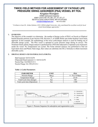
- 1. 1 TWICE-YIELD METHOD FOR ASSESSMENT OF FATIGUE LIFE PRESSURE SWING ADSORBER (PSA) VESSEL BY FEA. Kingston Rivington ASME Authorized Inspector ASNT Level 3 RT, PT, MT, UT, VT, ET, LT ISO 9712 Level 3 PAUT/TOFD, API 510,570,653 rivington24@gmail.com Ref: # 9-2-2020 “A tribute to Late Dr. Arthur Kalnins (1931-2020) Lehigh University, who contributed his excellent work for local strain-based fatigue approaches “ ------------------------------------------------------------------------------------------------------------------------------------------- 1. OVERVIEW: The objective of the example is to determine the number of design cycles of PSA’s at Nozzle to Elliptical head & Knuckle portions as per Section VIII, Division 2³, of ASME Boiler and Arthur Kalnins² local strain approach. In this example, the methodology of the twice yield fatigue analysis is used for finding out of allowable design cycles. The PSA vessel is operated at cyclic pressure range during its service. The Nonlinear Elastic plastic fatigue analysis is performed for a PSA that subjected to a repeated cycle of pressure inside the vessel. No Temperatures are cycled. The Finite element analysis was performed to find out Equivalent stress and Plastic Stain range, then values are substitute into Div,2 formulae to obtain maximum allowable cycles. 2. ORGINAL DESIGN AND MATERIAL DATA FOR PSA Shell material: SA516 Gr70 Ellipsoidal Head material 2:1: SA516 Gr70 Nozzle Pipe: SA350LF2 Cl 1 Nozzle Flange: SA 350 LF2 Cl.1 Table 1. Cyclic Parameters PARAMETER UNIT PSA Pressure Range Bar.g 4 –70 (7.0 Mpa) Temperature Range ºC 25-45 Total Cycle time (design) Sec 540 Total cycle time (Operation) Sec 1100 Figure 1: Pressure Sequence for adsorption and regeneration cycle.
- 2. 2 Figure-2 Design drawing details for PSA 3.0 NOMENCLATURE nc s s = material parameter for the cyclic stress–strain curve model σa = total stress amplitude. σr = total stress range Kc s s = material parameter for the cyclic stress–strain curve model Δεpeq, k = equivalent plastic strain range for the kth loading condition or cycle. Δεeff , k = Effective Strain Range for the kth cycle. ΔSp k = equivalent stress Range Eya,k = value of modulus of elasticity of the material at the point under consideration ɛtr = total true strain range. ɛ pr = Plastic strain range. Salt =effective alternating equivalent stress amplitude 4.0 MATERIAL PROPERTIES FOR STRESS ANALYSIS According to 2019 Div. 2, paragraph 5.5.4.1(c ), a stabilized cyclic stress-strain curve shall be used. In this example, the cyclic curves provided in 2019 Div. 2, Part 3, Annex 3.D, paragraph 3.D.4, will be used. The cyclic curve is defined by equation (1).
- 3. 3 The ɛta , total true strain amplitude to be cycled, The above equation is Ramberg-Osgood (R-O) format of the cyclic curve of equation (1) is not of the form that used in typical finite element programs that require a separation of elastic and elastic-plastic behaviour at a specified yield stress. Equation (1) gives no such yield stress separation. To find out the yield stress the following two methods are followed as described Arthur Kalnins² 1. Method A : To approximate this yield stress and modify the form of the curve, an offset of plastic strain, offset, (2.0e-5) is assumed and a line is drawn along the elastic slope of Ramberg-Osgood (R-O). The intersection of this line and the cyclic stress-strain curve is taken as the yield stress Figure-3 Ramberg-Osgood yield stress by curve shift method 2.Method B: The yield stress is calculated also from formula approach equation (2) For this example, the Method B formula approach has been chosen to find out yield stress. ncss = 0.126 Table 3-D.2M Cyclic Stress–Strain Curve Data Kcss = 693 Mpa Table 3-D.2M Cyclic Stress–Strain Curve Data offset= 2.0e-5 Table 3-D.1M Cyclic Stress–Strain Curve Data σy Yield stress = 177.25 Mpa
- 4. 4 For the Twice-Yield Method, the curves are then converted to the hysteresis loop stress and strain curve form (strain range versus stress range). The plastic strain range is related to the stress range by the following equation (3) Table 2: Stress range versus plastic strain range Stress range (Mpa) Ey ncss Kcss εoffset Plastic Strain Range 355 1.98E+05 0.126 693 2.00E-05 0.00E+00 370 1.98E+05 0.126 693 2.00E-05 1.61E-05 380 1.98E+05 0.126 693 2.00E-05 2.93E-05 390 1.98E+05 0.126 693 2.00E-05 4.52E-05 400 1.98E+05 0.126 693 2.00E-05 6.42E-05 410 1.98E+05 0.126 693 2.00E-05 8.67E-05 420 1.98E+05 0.126 693 2.00E-05 1.13E-04 430 1.98E+05 0.126 693 2.00E-05 1.45E-04 440 1.98E+05 0.126 693 2.00E-05 1.82E-04 450 1.98E+05 0.126 693 2.00E-05 2.25E-04 460 1.98E+05 0.126 693 2.00E-05 2.76E-04 470 1.98E+05 0.126 693 2.00E-05 3.35E-04 480 1.98E+05 0.126 693 2.00E-05 4.03E-04 490 1.98E+05 0.126 693 2.00E-05 4.81E-04 500 1.98E+05 0.126 693 2.00E-05 5.72E-04 510 1.98E+05 0.126 693 2.00E-05 6.76E-04 520 1.98E+05 0.126 693 2.00E-05 7.96E-04 530 1.98E+05 0.126 693 2.00E-05 9.32E-04 540 1.98E+05 0.126 693 2.00E-05 1.09E-03 550 1.98E+05 0.126 693 2.00E-05 1.26E-03 560 1.98E+05 0.126 693 2.00E-05 1.46E-03 The Table 2 Stress range versus plastic strain range values are taken into material model. 5.0 MODEL AND LOADING The axisymmetric model 2D was taken from Example as 3D models are time consumed and complicated. The pressure load was modified to 7 Mpa (load at the cycle end point) and the nozzle thrust load(14 Mpa) was adjusted accordingly. The boundary conditions are X=0 ,Y=0.The multilinear Kinematic hardening Ansys workbench¹ model has been chosen. Figure 4.PSA model Figure 5. 2D model
- 5. 5 Figure 6. Boundary condition 6.0 DETERMINATION OF EFFECTIVE STRAIN RANGE BY TWICE-YIELD METHOD The method is explained well by A. Kalnins² in his paper that if in the input the loading is specified as the loading range, and the cyclic stress range-strain range curve is used for the material model, then in the output the stress components are the stress component ranges and the strain components are the strain component ranges. Thus, in one FEA load step, for which the loading is specified from zero to that of the loading range, the output provides the stress and strain ranges that are needed for fatigue analysis Figure 4 : Twice Yield method with single load step 7.0 DETERMINATION OF DESIGN CYCLES
- 6. 6 Figure 7. Von mises Equivalent stress range Figure 8. Equivalent plastic strain range a). To find out Effective Strain Ranges ΔSp k = equivalent stress (values obtained from Ansys output) Δεpeq, k = equivalent plastic strain range (values obtained from Ansys output) Eya,k = value of modulus of elasticity of the material Table-3 Component Location Eya,k ΔSp k Δεpeq, k Δεeff , k Nozzle Inside Radius 1.98E+05 515.84 8.34E-04 3.44E-03 Knuckle inside radius 1.98E+05 363.69 1.00E-05 1.85E-03
- 7. 7 b. Determine the effective alternating equivalent stress for the cycle. Table- 4 Component Location Eya,k Δεeff , k Salt,K Nozzle Inside Radius 1.98E+05 3.44E-03 3.41E+02 Knuckle inside radius 1.98E+05 1.85E-03 1.83E+02 C. Determine the permissible number of cycles, Nk , for the alternating equivalent stress computed in Step b. Fatigue curves based on the materials of construction are provided in ASME Division VIII Div 2 Annex 3-F, 3-F.1, For Carbon, Low Alloy, Series 4XX, High Alloy, and High Tensile Strength Steels for temperatures not exceeding 371°C (700°F). The fatigue curve values may be interpolated for intermediate values of the ultimate tensile strength. ET = the material modulus of elasticity at the cycle temperature (1) For σuts ≤ 552 MPa (80 ksi) (see Figures 3-F.1M and 3-F.1) and for 48 MPa (7 ksi) ≤ Sa ≤ 3 999 MPa (580 ksi) 10ᵞ = 32.24 The above equation can be used. The design number of design cycles, N, can be computed from eq. (3-F.21) based on the parameter X calculated for the applicable material Table- 5 Component Location ET Sa Y X N cycles Nozzle Inside Radius 1.98E+05 3.41E+02 1.68E+00 3.70E+00 5032 Knuckle inside radius 1.98E+05 1.83E+02 1.41E+00 4.53E+00 33800 8.0 CONCLUSION Refer from table -5, nozzle to ellipsoidal head junction, would limit the design cycle life of PSA is 5032 cycles. References 1.ANSYS workbench (version 19.2) [FEA software] 2.Twice-Yield Method for Assessment of Fatigue Caused by Fast Thermal Transient According To 2007 Section Viii-Division 2 by Arthur Kalnins. 3.ASME Boiler & Pressure Vessel Code, Section VIII Div.2 2019 edition. 4.ASME PTB-3-2013