Solution Manual for Introduction to Finite Element Analysis and Design Author(s) : Nam-Ho Kim and Bhavani V. Sankar This solution manual include all problems (Chapters 0 to 8) of textbook.

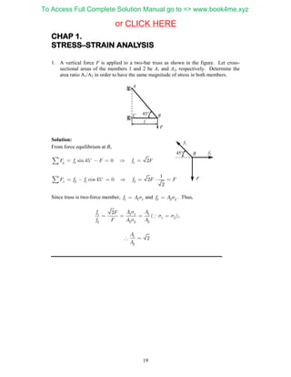
1. 19
CHAP 1.
STRESS–STRAIN ANALYSIS
1. A vertical force F is applied to a two-bar truss as shown in the figure. Let cross-
sectional areas of the members 1 and 2 be A1 and A2, respectively. Determine the
area ratio A1/A2 in order to have the same magnitude of stress in both members.
Solution:
From force equilibrium at B,
1 1sin 45 0 2yF f F f F     
2 1 2
1
cos 45 0 2
2
xF f f f F F       
Since truss is two-force member, 1 1 1f A  and 2 2 2f A  . Thus,
1 1 1 1
1 2
2 2 2 2
2
( )
f A AF
f F A A

 

    ,
1
2
2
A
A
 
l
C B
A
45
F
45
f1
f2
F
B
CLICK HEREor
To Access Full Complete Solution Manual go to => www.book4me.xyz

2. 20 Finite Element Analysis and Design
2. The stress at a point P is given below. The direction cosines of the normal n to a
plane that passes through P have the ratio nx:ny:nz = 3:4:12. Determine (a) the
traction vector T(n)
; (b) the magnitude T of T(n)
; (c) the normal stress n; (d) the shear
stress n; and (e) the angle between T(n)
and n.
Hint: Use 2 2 2
1x y zn n n   .
13 13 0
[ ] 13 26 13
0 13 39

 
 
   
    
Solution:
(a) First, we need unit normal vector n:
  2 2 2
3 0.2308
1
4 0.3077
3 4 12 12 0.9231
                   
                 
n
Then, the traction vector on this plane becomes
 ( )
13 13 0 0.2308 7
13 26 13 0.3077 1
0 13 39 0.9231 40
                                                      
n
T n
(b) Since T(n)
is a vector, its magnitude can be obtained using the norm as
( ) ( )2 ( )2 ( )2 2 2 2
7 ( 1) ( 40) 40.6202n n n n
x y zT T T T        
(c)    ( )
0.2308
7 1 40 0.3077 35.6154
0.9231
n
            
     
n
T n
(d)
2
( ) 2 2 2
40.6202 ( 35.6154) 19.5331n n      n
T
(e)  ( ) ( )
cosn   n n
T n T
1 0
( )
cos 2.64 151.3n
n
T

 
         

3. CHAP 1 Stress-Strain Analysis 21
3. At a point P in a body, Cartesian stress components are given by σxx = 80 MPa, σyy =
−40 MPa, σzz = −40 MPa, and τxy = τyz = τzx = 80 MPa. Determine the traction vector,
its normal component, and its shear component on a plane that is equally inclined to
all three coordinate axes.
Hint: When a plane is equally inclined to all three coordinate axes, the direction
cosines of the normal are equal to each other.
Solution:
The unit normal in this case is:
 
1 0.577
1
1 0.577
3
1 0.577
                   
               
n
The traction vector in this direction becomes
   
( )
80 80 80 0.577 138.56
80 40 80 0.577 69.28 MPa
80 80 40 0.577 69.28
                                                        
n
T n
The normal component of the traction vector is
   ( )
0.577
138.56 69.28 69.28 0.577 160 MPa
0.577
n
         
     
n
T n
The shear component of the traction vector is:
2
( ) 2 2 2
169.71 160 56.58 MPan n     n
T

4. 22 Finite Element Analysis and Design
4. If xx = 90 MPa, yy = −45 MPa, xy = 30 MPa, and zz = xz = yz = 0, compute the
surface traction T(n)
on the plane shown in the figure, which makes an angle of  =
40 with the vertical axis. What are the normal and shear components of stress on
this plane?
Solution:
Unit normal vector:  cos(40) sin(40) 0T
n
Traction vector: ( )
90 30 0 .776 88.23
[ ] 30 45 0 .643 5.94 MPa
0 0 0 0 0
                                                    
n
T n
Normal stress: ( )
63.77MPan   n
T n
Shear stress:
2
( ) 2
61.27MPan n   n
T
n
xxxx
yy
yy
xy
xy
xy
xy


5. CHAP 1 Stress-Strain Analysis 23
5. Find the principal stresses and the corresponding principal stress directions for the
following cases of plane stress.
(a) σxx = 40 MPa, σyy = 0 MPa, τxy = 80 MPa
(b) σxx = 140 MPa, σyy = 20 MPa, τxy = −60 MPa
(c) σxx = −120 MPa, σyy = 50 MPa, τxy = 100 MPa
Solution:
(a) The stress matrix becomes
40 80
MPa
80 0
xx xy
xy yy
 
 
   
      
      
To find the principal stresses, the standard eigen value problem can be written as
  0   I n
The above problem will have non-trivial solution when the determinant of the coefficient
matrix becomes zero:
40 80
0
80 0
xx xy
xy yy
   
   
 
 
 
The equation of the determinant becomes:
     2
40 80 80 40 6400 0           
The above quadratic equation yields two principal stresses, as
1 102.46MPa  and 2 62.46MPa   .
To determine the orientation of the first principal stresses, substitute 1 in the original
eigen value problem to obtain
40 102.46 80 0
80 0 102.46 0
x
y
n
n
                                
Since the determinant is zero, two equations are not independent
62.46 80x yn n   and 80 102.46x yn n    .
Thus, we can only get the relation between nx and ny. Then using the condition |n| = 1 we
obtain

6. 24 Finite Element Analysis and Design
(1)
0.788
0.615
x
y
n
n
            
         
To determine the orientation of the second principal stress, substitute 2 in the original
eigen value problem to obtain
40 62.46 80 0
80 0 62.46 0
x
y
n
n
                                
102.46 80x yn n    and 80 62.46x yn n    .
Using similar procedures as above, the eigen vector of 2 can be obtained as
(2)
0.615
0.788
x
y
n
n
            
         
Note that if n is a principal direction, −n is also a principal direction
(b) Repeat the procedure in (a) to obtain
1 164.85MPa  and 2 4.85MPa   .
(1)
0.924
0.383
x
y
n
n
            
         
and
(2)
0.383
0.924
x
y
n
n
            
         
(c) Repeat the procedure in (a) to obtain
1 96.24 MPa  and 2 166.24 MPa   .
(1)
0.420
0.908
x
y
n
n
            
         
and
(2)
0.908
0.420
x
y
n
n
            
         
Note that for the case of plane stress 3=0 is also a principal stress and the corresponding
principal stress direction is given by n(3)
=(0,0,1)

7. CHAP 1 Stress-Strain Analysis 25
6. If the minimum principal stress is −7 MPa, find σxx and the angle that the principal
stress axes make with the x and y axes for the case of plane stress illustrated
Solution:
With unknown x-component, the eigen value problem can be written as
56 0
56 21 0
xx x
y
n
n
 

                                  
The principal stresses can be determined by making the determinant zero
2
56
0 ( )(21 ) 56 0
56 21
xx
xx
 
  

 
     
 
Since −7 MPa is one of the roots of the above equation, we can find xx by substituting
in the above equation as
2
( 7)(21 7) 56 0xx    
By solving the above equation, we can get 105MPaxx  . Then, the other principal
stress can be found from the original determinant, as
1 2133MPa 7 MPa   
Principal direction for the first principal stress: From the original eigen value
problem,
1 1
1 1
(105 133) 56 0
56 (21 133) 0
x y
x y
n n
n n
  
   
The solution of the above equations is not unique. By putting |n1
| = 1, we have
{ 0.8944, 0.4472} 1
n  , which is principal direction corresponding to 1
Principal direction for the second principal stress: From the original eigen value
problem,
x
y
21 MN/m2
56 MN/m2
xx

8. 26 Finite Element Analysis and Design
2 2
2 2
(105 7) 56 0
56 (21 7) 0
x y
x y
n n
n n
  
   
The solution of above equations is 2
{ 0.4472, 0.8944}  n , which is principal
direction corresponding to 2 . Two principal directions are plotted on the following
graph. Note that the two principal directions are perpendicular each other.
y
x
n2
n1
n1'
n2'
-26.57o
135.43o

9. CHAP 1 Stress-Strain Analysis 27
7. Determine the principal stresses and their associated directions, when the stress
matrix at a point is given by
1 1 1
[ ] 1 1 2 MPa
1 2 1
 
 
   
 
  

Solution:
Use the Eq. (0.46) of Chapter 0 with the coefficients of I1=3, I2= −3, and I3 = −1,
3 2
3 3 1 0     
By solving the above cubic equation using the method described in Section 0.4,
1 2 33.73MPa, 0.268 MPa, 1.00MPa     
(a) Principal direction corresponding to 1:
1 1 1
1 1 1
1 1 1
(1 3.7321) 0
(1 3.7321) 2 0
2 (1 3.7321) 0
x y z
x y z
x y z
n n n
n n n
n n n
   
   
   
Solving the above equations with |n1
| = 1 yields
{ 0.4597, 0.6280, 0.6280}   1
n
(b) Principal direction corresponding to 2:
1 1 1
2 2 2
2 2 2
(1 0.2679) 0
(1 0.2679) 2 0
2 (1 0.2679) 0
x y z
x y z
x y z
n n n
n n n
n n n
   
   
   
Solving the above equations with |n2
| = 1 yields
2
{ 0.8881, 0.3251, 0.3251} n  
(c) Principal direction corresponding to 3:
3 3 3
3 3 3
3 3 3
(1 1) 0
(1 1) 2 0
2 (1 1) 0
x y z
x y z
x y z
n n n
n n n
n n n
   
   
   
Solving the above equations with |n2
| = 1 yields

10. 28 Finite Element Analysis and Design
3
{0, 0.7071, 0.7071} n 

11. CHAP 1 Stress-Strain Analysis 29
8. Let x′y′z′ coordinate system be defined using the three principal directions obtained
from Problem 7. Determine the transformed stress matrix [σ]x′y′z′ in the new
coordinates system.
Solution:
The three principal directions in Problem 6 can be used for the coordinate transformation
matrix:
(1) (2) (3)
(1) (2) (3)
(1) (2) (3)
0.460 0.888 0
0.628 0.325 0.707
0.628 0.325 0.707
x x x
y y y
z z z
n n n
n n n
n n n
      
                   
N
To determine the stress components in the new coordinates we use Eq. (1.30):
1 0 0
0 .268 0
0 0 3.732
T
x y z  
  
                  
 
  
N N 
Note that the transformed stress matrix is a diagonal matrix with the original principal
stresses on the diagonal.

12. 30 Finite Element Analysis and Design
9. For the stress matrix below, the two principal stresses are given as σ3 = −3 and σ1 = 2,
respectively. In addition, the two principal stress directions corresponding to the two
principal stresses are also given below.
1 0 2
[ ] 0 1 0
2 0 2
 
 
   
   
 , 1
2
5
0
1
5
 
 
 
 
 
 
 
 
  
n and 3
1
5
0
2
5
 
 
 
 
 
 
 
 
  
n
(a) What is the normal and shear stress on a plane whose normal vector is parallel to
(2, 1, 2)?
(b) Calculate the missing principal stress σ2 and the principal direction n2
.
(c) Write stress matrix in the new coordinates system that is aligned with n1
, n2
, and
n3
.
Solution:
(a) Normal vector: 1
3
{2 1 2}T
n
Traction vector ( ) 1
3
2
0
                
n
T n
The normal component of the stress vector on the plane can be calculated
( )
2
( ) 2
1.4444
1.4229
n
n n

 
  
  
n
n
T n
T
(b) Using Eq. (0.46) of Chapter 0, the eigen values are governed by
3 2
1 2 3 0I I I     
We can find the coefficients of the above cubic equation from Eq. (0.47) by I1 = 0, I2 =
−7, and I3 = −6. Thus, we have
3 2
7 6 ( 1)( 6) 0          
Thus, the missing principal stress is 2 1  .
Since three principal directions are mutually orthogonal, the third principal direction
can be calculated using the cross product. To establish a defined sign convention for the
principal axes, we require them to form a right-handed triad. If n1
and n3
are unit vectors
that define the directions of the first and third principal axes, then the unit vector n2
for
the second principal axis is determined by the right-hand rule of the vector multiplication.
Thus we have

13. CHAP 1 Stress-Strain Analysis 31
2 3 1
{0 1 0}T
  n n n
(c) Coordinate transformation matrix can be obtained from three principal directions as
2 1
0
5 5
0 1 0
1 2
0
5 5
 
 
 
            
 
 
  
1 2 3
N n n n
The stress matrix at the transformed coordinates becomes
2 1 2 1
0 01 0 2 2 0 0
5 5 5 5
0 1 0 0 1 0 0 1 0 0 1 0
1 2 2 0 2 1 2 0 0 3
0 0
5 5 5 5
T
   
                                                          
      
N N

14. 32 Finite Element Analysis and Design
10. With respect to the coordinate system xyz, the state of stress at a point P in a solid is
20 0 0
[ ] 0 50 0 MPa
0 0 50
  
   
 
  

(a) m1
, m2
and m3
are three mutually perpendicular vectors such that m1
makes 45º
with both x- and y-axes and m3
is aligned with the z-axis. Compute the normal
stresses on planes normal to m1
, m2
, and m3
.
(b) Compute two components of shear stress on the plane normal to m1
in the
directions m2
and m3
.
(c) Is the vector n = {0, 1, 1}T
a principal direction of stress? Explain. What is the
normal stress in the direction n?
(d) Draw an infinitesimal cube with faces normal to m1
, m2
and m3
and display the
stresses on the positive faces of this cube.
(e) Express the state of stress at the point P with respect to the x′y′z′ coordinates
system that is aligned with the vectors m1
, m2
and m3
?
(f) What are the principal stress and principal directions of stress at the point P with
respect to the x′y′z′ coordinates system? Explain.
(g) Compute the maximum shear stress at the point P. Which plane(s) does this
maximum shear stress act on?
Solution:
(a)
1 2 31 1
(1,1,0) ( 1,1,0) (0,0,1)
2 2
T T T
   m m m
1 1
2 2
3 3
1 1
2 2
3 3
[ ] 15 MPa
[ ] 15 MPa
[ ] 50 MPa
 
 
 
   
   
   
m m
m m
m m
m m
m m
m m
(b)
1
( ) 1 1
[ ] { 20 50 0}
2
T
   m
T m
x
y
z
m1
m2
m3
P

15. CHAP 1 Stress-Strain Analysis 33
1
1 2
1
1 3
( ) 2
( ) 3
35 MPa
0 MPa


  
  
m
m m
m
m m
T m
T m
(c) Yes,
1
(0,1,1)
2
n
( )
50 1
1 1
[ ] 50 50 1 50
2 2
0 0

                       
               
n
T n n
Since T(n)
// n, n is a principal direction with principal stress = 50 MPa.
(d)
(e)
0.707 0.707 0 20 0 0
-0.707 0.707 0 0 50 0
0 0 1 0 0 50
0.707 -0.707 0
0.707 0.707 0
0 0 1
T
x y z
N N   
      
                      
   
      
 
 
  
 
  
15 35 0
[ ] 35 15 0 MPa
0 0 50
x y z   
 
 
   
 
  
(f) Principal stresses = 50, 50, and −20 MPa
3 1
(1, 1,0)
2
 n
n1
and n2
are any two perpendicular unit vectors that is on the plane perpendicular to n3
.
15
15
3535
-20
m1
m2
m3

16. 34 Finite Element Analysis and Design
(g) The maximum shear stress occurs on a plane whose normal is at 45o
from the
principal stress direction. Since 1 = 2, all directions that are 45o
from x-axis (3 axis)
will have the maximum shear stress whose value is
1 3
max 35 MPa
2
 


 
The maximum shear stress planes are in the shape of a cone whose axis is parallel to x-
axis and has an angle of 45o
.

17. CHAP 1 Stress-Strain Analysis 35
11. A solid shaft of diameter d = 5 cm, as shown in the figure, is subjected to tensile
force P = 13,000 N and a torque T = 6,000 Ncm. At point A on the surface, what is
the state of stress (write in matrix form), the principal stresses, and the maximum
shear stress? Show the coordinate system you are using.
Solution:
Let us establish a coordinate system as shown in the figure. The axial force will cause
normal stress xx, while the torque will cause shear stress xy. Their magnitudes are
6.62 MPa
P
A

2.44 MPa
T r
J


Then, the stress matrix becomes
6.62 2.44 0
[ ] 2.44 0 0 MPa
0 0 0
A
  
   
 
  
By solving the eigen value problem, the principal stress can be obtained as
1 2 37.43, 0, 0.81 MPa     
Maximum shear stress is
1 2
max 4.11 MPa
2
 


 
P
T
 A
A
y
z

18. 36 Finite Element Analysis and Design
12. If the displacement field is given by
2 2
2
2
2
2 ( )
2
x
y
z
u x y
u y x y z
u z xy
      
   
(a) Write down 3×3 strain matrix.
(b) What is the normal strain component in the direction of (1,1,1) at point (1,–3,1)?
Solution:
(a) 3×3 symmetric strain matrix can be calculated from its definition as
2
2( ) 0
0 2
x y z y
y z x y
y z
   
        
    

In addition, the unit normal vector in the direction of (1, 1, 1) is
1
{1 1 1}
3
T
n
b) Thus, the normal component of strain is
1 2
(2 2 2 2 )
3 3
x y z y y z x y y z y               n n
Thus, the normal component of strain reduces as the y-coordinate of a point increases. At
point (1, −3, 1), y = −3
3
2y
     n n .

19. CHAP 1 Stress-Strain Analysis 37
13. Consider the following displacement field in a plane solid:
( , ) 0.04 0.01 0.006
( , ) 0.06 0.009 0.012
u x y x y
v x y x y
  
  
(a) Compute the strain components xx, yy, and xy. Is this a state of uniform strain?
(b) Determine the principal strains and their corresponding directions. Express the
principal strain directions in terms of angles the directions make with the x-axis.
(c) What is the normal strain at Point O in a direction 45o
to the x-axis?
Solution:
(a) Strain components:
0.01xx
u
x


  

0.012yy
v
y


 

0.009 0.006 0.015xy
v u
x y

 
    
 
Yes, this is a state of uniform strain, because the strains are independent of position x,y,z.
(b) Principal strains and principal directions.
1
0.0075
2xy xy  
0.01 0.0075
0.0075 0.012
xx xy
xy yy
 
 
   
       
      

Find the eigen values (principal strains) and eigen vectors (principal direction) by solving
the eigen value problem:
0.01 0.0075 0
0.0075 0.012 0
x
y
n
n


                                 
The above equation yields two principal strains: 1 = 1 = 0.01231 and 2 = 2 =
0.01431. The principal direction corresponding to the first principal strain is
 (1)
0.9556 0.2948 n ,
The angle the direction makes with the x-axis can be found from the relation
cos 0.9556,sin 0.2948     . Solving 163o
 
The principal direction corresponding to the second principal strain is

20. 38 Finite Element Analysis and Design
 (2)
0.2948 0.9556n ,
and the angle is found to be 73o
 
(c)
Strain at point O
0.01 0.0075
0.0075 0.012
 
   
  
 ,
direction vector
1
2
1
2
        
      
n
Thus the normal strain in the direction of n becomes
45
1 1
0.01 0.0075
2 2 0.0085
1 0.0075 0.012 1
2 2
o
T

                                                 
n n