Download to read offline
![Large-Scale Graph Mining is Everywhere
Symbolic Networks: Human
Brain: 100 billion neuron
Protein Interactions
[genomebiology.com]
Social Networks[Moody ’01]
(Facebook: 1 billion users) Cyber Security ( 15 billion log
entries / day for large enterprise)
Cybersecurity
Medical Informatics
Data Enrichment
Social Networks
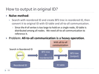
Symbolic Networks
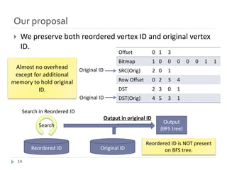
WWW[lumeta.com]
(1 trillion unique URL)
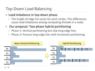
2](https://image.slidesharecdn.com/graph500-bigdata2016-slides-170110031013/85/Extreme-Scale-Breadth-First-Search-on-Supercomputers-2-320.jpg)
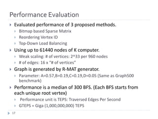
![Graph500 Benchmark [http://www.graph500.org/]
} One of our major targets is Graph500 benchmark.
} Benchmark for Big Data (data intensive) applications.
} BFS is a main kernel for ranking.
} K computer is #1 using our result.
Graph500 Latest Ranking
4](https://image.slidesharecdn.com/graph500-bigdata2016-slides-170110031013/85/Extreme-Scale-Breadth-First-Search-on-Supercomputers-4-320.jpg)
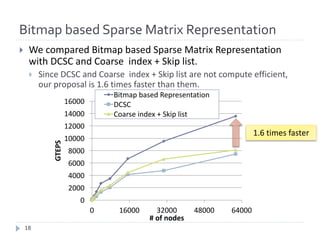
![Direction Optimization [Beamer, ’11-12]
} Direction optimization is an fast BFS algorithm which switches
direction (Top-Down and Bottom-Up) for each searching level.
} Direction optimization is effective for small diameter graphs.
} Scale free networks and small world networks are small diameter
graphs.
} The target of Graph500 benchmark is also small diameter
graph and direction optimization is effective.
Frontier
Neighbors
Level k
Level k+1
Frontier
Level k
Level k+1
Neighbors
Top-Down Bottom-Up
6](https://image.slidesharecdn.com/graph500-bigdata2016-slides-170110031013/85/Extreme-Scale-Breadth-First-Search-on-Supercomputers-6-320.jpg)
![RelatedWork
} Distributed BFS with Top-Down only:
} 2D Partitioning BFS on BlueGene/L [Yoo ‘05]
} Proposed Distributed Memory BFS on Large Distributed Memory
} Comparison of 1D Partitioning and 2D Partitioning [Buluc ‘11]
} Distributed Memory BFS on Commodity Machine (Intel CPU and
Infiniband network) [Satish ‘12]
} Distributed BFS with Direction Optimization
} 2D Partitioning BFS with Direction Optimization [Beamer ’13]
} Our proposed BFS is based on their BFS.
} 1D Partitioning BFS with Direction Optimization and Load Balancing.
[Checconi ‘14]
} This is very scalable and they achieved 23751 GTEPS on BlueGene/Q 98304 Nodes.
} They Proposed novel sparse matrix representation “Coarse index + Skip list”.
However, our bitmap based sparse matrix representation is more efficient.
8](https://image.slidesharecdn.com/graph500-bigdata2016-slides-170110031013/85/Extreme-Scale-Breadth-First-Search-on-Supercomputers-8-320.jpg)
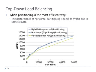
![Bitmap based Sparse Matrix Representation
SRC 0 0 6 7
DST 4 5 3 1
・Edge List
Offset 0 1 3
Bitmap 1 0 0 0 0 0 1 1
Row Offset 0 2 3 4
DST 4 5 3 1
・Bitmap base Sparse Matrix
Only consumes 8 bits
} Structure
} Row Offset: Skip vertices that has no edges (same as DCSC)
} Bitmap: one bit for each vertex: represents the vertex has at least one edge (set
bit) or not (not set bit).
} Offset: Supplemental array for faster computing: Represents cumulative # of set
bits from the beginning of bitmap to the corresponding word boarder.
} How to compute the row offset index of a given vertex?
} Row offset index = Offset[w] + popcount(Bitmap[w]&mask)
} Where w = v / 64, mask = (1 << (v % 64)) – 1, v is index of a given vertex.
} This is no loop. Therefore, this is an O(1) operation, which is same as CSR.
In this example, 1 word is 4 bit.
Partitioned Graph Adjacency Matrix: 8 Vertex and 4 Edge
Example
11](https://image.slidesharecdn.com/graph500-bigdata2016-slides-170110031013/85/Extreme-Scale-Breadth-First-Search-on-Supercomputers-11-320.jpg)
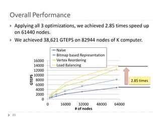


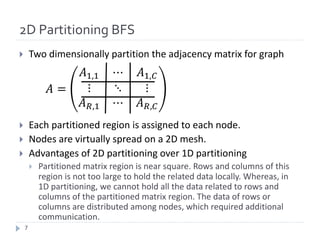
The document discusses advancements in efficient breadth-first search (BFS) algorithms for large-scale supercomputers, focusing on techniques such as bitmap-based sparse matrix representation, vertex reordering, and load balancing. The proposed methods resulted in a significant performance increase, achieving 38,621 giga traversed edges per second on the K computer, which contributes to its top ranking in the Graph500 benchmark. The authors address challenges in partitioning and accessing hyper sparse matrices while introducing innovative solutions that enhance computational efficiency.


![Data Structures - Lecture 10 [Graphs]](https://cdn.slidesharecdn.com/ss_thumbnails/datastructures-lecture10graphs-150305004608-conversion-gate01-thumbnail.jpg?width=640&height=640&fit=bounds)


![7.__Developing_a_Research_Proposal[1].pptx](https://cdn.slidesharecdn.com/ss_thumbnails/7-260131073037-df92dd7d-thumbnail.jpg?width=640&height=640&fit=bounds)


![제 23회 보아즈(BOAZ) 빅데이터 컨퍼런스 - [MBOAX] : ABSA를 활용한 소비자 반응 분석 기반 운영 효율화 대시보드 설계](https://cdn.slidesharecdn.com/ss_thumbnails/3-1boaz23rdconferencemboax-260203102709-9d519923-thumbnail.jpg?width=640&height=640&fit=bounds)


