Explain the use of fuzzy neural network

1. 206
Chapter 3
Fuzzy Neural Networks
3.1 Integrationoffuzzylogicandneuralnet-
works
Hybrid systems combining fuzzy logic, neural networks, genetic algorithms,
and expert systems are proving their effectiveness in a wide variety of real-
world problems.
Every intelligent technique has particular computational properties (e.g. abil-
ity to learn, explanation of decisions) that make them suited for particular
problems and not for others. For example, while neural networks are good at
recognizing patterns, they are not good at explaining how they reach their
decisions. Fuzzy logic systems, which can reason with imprecise information,
are good at explaining their decisions but they cannot automatically acquire
the rules they use to make those decisions. These limitations have been a
central driving force behind the creation of intelligent hybrid systems where
two or more techniques are combined in a manner that overcomes the lim-
itations of individual techniques. Hybrid systems are also important when
considering the varied nature of application domains. Many complex do-
mains have many different component problems, each of which may require
different types of processing. If there is a complex application which has
two distinct sub-problems, say a signal processing task and a serial reason-
ing task, then a neural network and an expert system respectively can be
used for solving these separate tasks. The use of intelligent hybrid systems
is growing rapidly with successful applications in many areas including pro-

2. 207
Decisions
Perception as
neural inputs
(Neural
outputs)
Linguistic
statements
Learning
algorithm
Fuzzy
Interface
Neural
Network
cess control, engineering design, financial trading, credit evaluation, medical
diagnosis, and cognitive simulation.
While fuzzy logic provides an inference mechanism under cog-
nitive uncertainty, computational neural networks offer exciting
advantages, such as learning, adaptation, fault-tolerance, paral-
lelism and generalization.
To enable a system to deal with cognitive uncertainties in a man-
ner more like humans, one may incorporate the concept of fuzzy
logic into the neural networks.
The computational process envisioned for fuzzy neural systems is as follows.
It starts with the development of a ”fuzzy neuron” based on the understand-
ing of biological neuronal morphologies, followed by learning mechanisms.
This leads to the following three steps in a fuzzy neural computational pro-
cess
• development of fuzzy neural models motivated by biological neurons,
models of synaptic connections which incorporates fuzziness into neural
network,
development of learning algorithms (that is the method of adjusting
the synaptic weights)
Two possible models of fuzzy neural systems are
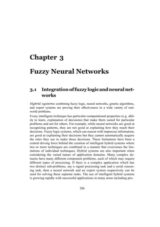
In response to linguistic statements, the fuzzy interface block provides
an input vector to a multi-layer neural network. The neural network can
be adapted (trained) to yield desired command outputs or decisions.
•
•
•

3. 208
Knowledge-base
Fuzzy
Inference
Neural
Inputs Neural outputs Decisions
Learning
algorithm
Neural
Network
Figure 3.1 The first model of fuzzy neural system.
• A multi-layered neural network drives the fuzzy inference mechanism.
Figure 3.2 The second model of fuzzy neural system.
Neural networks are used to tune membership functions of fuzzy systems
that are employed as decision-making systems for controlling equipment. Al-
though fuzzy logic can encode expert knowledge directly using rules with
linguistic labels, it usually takes a lot of time to design and tune the mem-
bership functions which quantitatively define these linquistic labels. Neural
network learning techniques can automate this process and substantially re-
duce development time and cost while improving performance.
In theory, neural networks, and fuzzy systems are equivalent in that they
are convertible, yet in practice each has its own advantages and disadvan-
tages. For neural networks, the knowledge is automatically acquired by the
backpropagation algorithm, but the learning process is relatively slow and
analysis of the trained network is difficult (black box). Neither is it possi-
ble to extract structural knowledge (rules) from the trained neural network,
nor can we integrate special information about the problem into the neural
network in order to simplify the learning procedure.
Fuzzy systems are more favorable in that their behavior can be explained
based on fuzzy rules and thus their performance can be adjusted by tuning
the rules. But since, in general, knowledge acquisition is difficult and also
the universe of discourse of each input variable needs to be divided into
several intervals, applications of fuzzy systems are restricted to the fields
where expert knowledge is available and the number of input variables is

4. 209
small.
To overcome the problem of knowledge acquisition, neural networks are ex-
tended to automatically extract fuzzy rules from numerical data.
Cooperative approaches use neural networks to optimize certain parameters
of an ordinary fuzzy system, or to preprocess data and extract fuzzy (control)
rules from data.
Based upon the computational process involved in a fuzzy-neuro system, one
may broadly classify the fuzzy neural structure as feedforward (static) and
feedback (dynamic).
A typical fuzzy-neuro system is Berenji’s ARIC (Approximate Reasoning
Based Intelligent Control) architecture [9]. It is a neural network modelofa
fuzy controller and learns by updating its prediction of the physical system’s
behavior and fine tunes a predefined control knowledge base.

5. 210
Figure 3.3 Berenji’s ARIC architecture.
This kind of architecture allows to combine the advantages of neural networks
and fuzzy controllers. The system is able to learn, and the knowledge used
within the system has the form of fuzzy IF-THEN rules. By predefining
these rules the system has not to learn from scratch, so it learns faster than
a standard neural control system.
ARIC consists of two coupled feed-forward neural networks, the Action-state
Evaluation Network (AEN) and the Action Selection Network (ASN). The
ASN is a multilayer neural network representation of a fuzzy controller. In
fact, it consists of two separated nets, where the first one is the fuzzy inference
part and the second one is a neural network that calculates p[t, t + 1], a
AEN
x v r (error signal)
Updating weights
Fuzzy inference network
ASN
x u(t)
u'(t)
x
p
Neural network
System state
Physical
System
Stochastic
Action
Modifier
Predict

6. 211
measure of confidence associated with the fuzzy inference value u(t +1), using
the weights of time t and the system state of time t +1. A stochastic modifier
combines the recommended control value u(t) of the fuzzy inference part and
the so called ”probability” value p and determines the final output value
uJ(t) = o(u(t), p[t, t + 1])
of the ASN. The hidden units zi of the fuzzy inference network represent
the fuzzy rules, the input units xj the rule antecedents, and the output
unit u represents the control action, that is the defuzzified combination of
the conclusions of all rules (output of hidden units). In the input layer the
system state variables are fuzzified. Only monotonic membership functions
are used in ARIC, and the fuzzy labels used in the control rules are adjusted
locally within each rule. The membership values of the antecedents of a
rule are then multiplied by weights attached to the connection of the input
unit to the hidden unit. The minimum of those values is its final input. In
each hidden unit a special monotonic membership function representing the
conclusion of the rule is stored. Because of the monotonicity of this function
the crisp output value belonging to the minimum membership value can be
easily calculated by the inverse function. This value is multiplied with the
weight of the connection from the hidden unit to the output unit. The output
value is then calculated as a weighted average of all rule conclusions.
The AEN tries to predict the system behavior. It is a feed-forward neural
network with one hidden layer, that receives the system state as its input and
an error signal r from the physical system as additional information. The
output v[t,tJ] of the network is viewed as a prediction of future reinforcement,
that depends of the weights of time t and the system state of time tJ, where
tJ may be t or t +1. Better states are characterized by higher reinforcements.
The weight changes are determined by a reinforcement procedure that uses
the ouput of the ASN and the AEN. The ARIC architecture was applied to
cart-pole balancing and it was shown that the system is able to solve this
task [9].

7. 212
3.1.1 Fuzzy neurons
Consider a simple neural net in Figure 3.4. All signals and weights are real
numbers. The two input neurons do not change the input signals so their
output is the same as their input. The signal xi interacts with the weight wi to
produce the product
pi = wixi, i = 1, 2.
The input information pi is aggregated, by addition, to produce the input
net = p1 + p2 = w1x1 + w2x2
to the neuron. The neuron uses its transfer function f , which could be a
sigmoidal function, f (x) = (1 + e−x)−1, to compute the output
y = f(net) = f(w1x1 + w2x2).
This simple neural net, which employs multiplication, addition, and sig-
moidal f , will be called as regular (or standard) neural net.
x1
w1
y = f(w1x1+w2x2)
x2 w2
Figure 3.4 Simple neural net.
If we employ other operations like a t-norm, or a t-conorm, to combine the
incoming data to a neuron we obtain what we call a hybrid neural net.
These modifications lead to a fuzzy neural architecture based on fuzzy arith-
metic operations. Let us express the inputs (which are usually membership
degrees of a fuzzy concept) x1, x2 and the weigths w1, w2 over the unit interval
[0, 1].
A hybrid neural net may not use multiplication, addition, or a sigmoidal
function (because the results of these operations are not necesserily are in
the unit interval).
Definition 3.1.1 A hybrid neural net is a neural net with crisp signals and
weights and crisp transfer function. However,

8. 213
we can combine xi and wi using a t-norm, t-conorm, or some other
continuous operation,
we can aggregate p1 and p2 with a t-norm, t-conorm, or any other
continuous function
• f can be any continuous function from input to output
We emphasize here that all inputs, outputs and the weights of a hybrid neural
net are real numbers taken from the unit interval [0, 1]. A processing element
ofa hybridneural netis calledfuzzy neuron. In thefollowingwepresent some
fuzzy neurons.
Definition 3.1.2 (AND fuzzy neuron [74, 75])
The signal xi and wi are combined by a triangular conorm S to produce
pi = S(wi, xi), i = 1,2.
Theinput information pi isaggregatedbyatriangular norm T toproducethe
output
y = AND(p1, p2) = T (p1, p2) = T (S(w1, x1), S(w2, x2))
of the neuron.
So, if T = min and S = max then the AND neuron realizes the min-max
composition
y = min{w1 ∨ x1, w2 ∨ x2}.
x1
w1
y = T(S(w1, x1), S(w2, x2))
x2 w2
Figure 3.5 AND fuzzy neuron.
•
•

9. 214
Definition 3.1.3 (OR fuzzy neuron [74, 75])
The signal xi and wi are combined by a triangular norm T to produce
pi = T (wi, xi), i = 1, 2.
The input information pi is aggregated by a triangular conorm S to produce
the output
y = OR(p1, p2) = S(p1, p2) = S(T(w1, x1),T (w2, x2))
of the neuron.
x1
w1
y = S(T(w1, x1), T(w2, x2))
x2 w2
Figure 3.6 OR fuzzy neuron.
So, if T = min and S = max then the AND neuron realizes the max-min
composition
y = max{w1 ∧ x1, w2 ∧ x2}.
The AND and OR fuzzy neurons realize pure logic operations on the member-
ship values. The role of the connections is to differentiate between particular
leveles of impact that the individual inputs might have on the result of aggre-
gation. We note that (i) the higher the value wi the stronger the impact of
xi on the output y of an OR neuron, (ii) the lower the value wi the stronger
the impact of xi on the output y of an AND neuron.
The range of the output value y for the AND neuron is computed by letting all
xi equal to zero or one. In virtue of the monotonicity property of triangular
norms, we obtain
y ∈ [T (w1, w2), 1]
and for the OR neuron one derives the boundaries
y ∈ [0, S(w1, w2)].

10. 215
Definition 3.1.4 (Implication-OR fuzzy neuron [37, 39])
The signal xi and wi are combined by a fuzzy implication operator I to produce
pi = I(wi, xi) = wi ← xi, i = 1, 2.
The input information pi is aggregated by a triangular conorm S to produce
the output
y = I(p1, p2) = S(p1, p2) = S(w1 ← x1, w2 ← x2)
of the neuron.
x1
w1
y=S(w1x1, w2  x2)
x2 w2
Figure 3.7 Implication-OR fuzzy neuron.
Definition 3.1.5 (Kwan and Cai’s fuzzy neuron [111])
The signal xi interacts with the weight wi to produce the product
pi = wixi, i = 1,...,n
Theinputinformationpi isaggregatedbyanagregationfunctionhtoproduce
the input of the neuron
z = h(w1x1, w2x2,..., wnxn)
the state of the neuron is computed by
s = f(z − θ)
where f is an activation function and θ is the activating threshold. And the
m outputs of the neuron are computed by
yj = gj(s), j = 1,...,m
wheregj, j =1,...,m arethe moutputfunctionsof theneuron whichrep-
resent the membership functions of the input pattern x1,x2,..., xn in all the
m fuzzy sets.

11. 216
w1 g1
h f
gm
wn
x1
y1
xn ym
Figure 3.8 Kwan and Cai’s fuzzy neuron.
Definition 3.1.6 (Kwan and Cai’s max fuzzy neuron [111])
The signal xi interacts with the weight wi to produce the product
pi = wixi, i = 1, 2.
The input information pi is aggregated by the maximum conorm
z = max{p1, p2} = max{w1x1, w2x2}
and the j-th output of the neuron is computed by
yj = gj(f(z − θ)) = gj(f(max{w1x1, w2x2} − θ))
where f is an activation function.
x1
Figure 3.9 Kwan and Cai’s max fuzzy neuron.
Definition 3.1.7 (Kwan and Cai’s min fuzzy neurons [111])
The signal xi interacts with the weight wi to produce the product
pi = wixi, i = 1, 2.
w1
z = max{w1x1, w2x2}
x2 w2

12. 217
The input information pi is aggregated by the minimum norm
y = min{p1, p2} = min{w1x1, w2x2}
and the j-th output of the neuron is computed by
yj = gj(f(z − θ)) = gj(f(min{w1x1, w2x2} − θ))
where f is an activation function.
x1
Figure 3.10 Kwan and Cai’s min fuzzy neuron.
It is well-known that regular nets are universal approximators, i.e. they can
approximate any continuous function on a compact set to arbitrary accuracy.
In a discrete fuzzy expert system one inputs a discrete approximation to the
fuzzy sets and obtains a discrete approximation to the output fuzzy set.
Usually discrete fuzzy expert systems and fuzzy controllers are continuous
mappings. Thus we can conclude that given a continuous fuzzy expert sys-
tem, or continuous fuzzy controller, there is a regular net that can uniformly
approximate it to any degree of accuracy on compact sets. The problem
with this result that it is non-constructive and only approximative. The
main problem is that the theorems are existence types and do not tell you
how to build the net.
Hybrid neural nets can be used to implement fuzzy IF-THEN rules in a
constructive way. Following Buckley & Hayashi [30], and, Keller, Yager &
Tahani [99] we will show how to construct hybrid neural nets which are
computationally equivalent to fuzzy expert systems and fuzzy controllers. It
should be noted that these hybrid nets are for computation and they do not
have to learn anything.
Though hybrid neural nets can not use directly the standard error backpropa-
gation algorithm for learning, they can be trained by steepest descent methods
w1
z = min{w1x1, w2x2}
x2 w2

13. 218
to learn the parameters of the membership functions representing the linguis-
tic terms in the rules (supposing that the system output is a differentiable
function of these parameters).
The direct fuzzification of conventional neural networks is to extend connec-
tion weigths and/or inputs and/or fuzzy desired outputs (or targets) to fuzzy
numbers. This extension is summarized in Table 3.1.
Fuzzy neural net Weights Inputs Targets
Type 1 crisp fuzzy crisp
Type 2 crisp fuzzy fuzzy
Type 3 fuzzy fuzzy fuzzy
Type 4 fuzzy crisp fuzzy
Type 5 crisp crisp fuzzy
Type 6 fuzzy crisp crisp
Type 7 fuzzy fuzzy crisp
Table 3.1 Direct fuzzification of neural networks.
Fuzzy neural networks (FNN) of Type 1 are used in classification problem of
a fuzzy input vector to a crisp class [84, 114]. The networks of Type 2, 3 and
4 are used to implement fuzzy IF-THEN rules [93, 95].
However, the last three types in Table 3.1 are unrealistic.
In Type 5, outputs are always real numbers because both inputs and
weights are real numbers.
In Type 6 and 7, the fuzzification of weights is not necessary because
targets are real numbers.
Definition 3.1.8 A regular fuzzy neural network is a neural network with
fuzzy signals and/or fuzzy weights, sigmoidal transfer function and all the
operations are defined by Zadeh’s extension principle.
Consider a simple regular fuzzy neural net in Figure 3.11. All signals and
weights are fuzzy numbers. The two input neurons do not change the input
•
•

14. 219
signals so their output is the same as their input. The signal Xi interacts
with the weight Wi to produce the product
Pi = WiXi, i = 1, 2.
where we use the extension principle to compute Pi. The input information
Pi is aggregated, by standard extended addition, to produce the input
net = P1 + P2 = W1X1 + W2X2
to the neuron. The neuron uses its transfer function f, which is a sigmoidal
function, to compute the output
Y = f(net) = f(W1X1 + W2X2)
where f(x) = (1 + e−x)−1 and the membership function of the output fuzzy
set Y is computed by the extension principle
.
Y (y) =
(W1X1 + W2X2)(f −1(y)) if 0 ≤ y ≤ 1
0 otherwise
where f−1(y) = ln y − ln(1 − y).
X1
W1
Y = f(W1X1+W2X2)
X2 W2
Figure 3.11 Simple regular fuzzy neural net.
Buckley and Hayashi [28] showed that regular fuzzy neural nets are mono-
tonic, i.e. if X1 ⊂ X1J and X2 ⊂ X2
J then
Y = f(W1X1 + W2X2) ⊂ Y J = f(W1X1
J
+ W2X2
J
).
where f is the sigmoid transfer function, and all the operations are defined
by Zadeh’s extension principle.
This means that fuzzy neural nets based on the extension principle might be
universal approximators only for continuous monotonic functions. If a fuzzy

15. 220
→ → ∞
∈ F ⊂
A 1
f(A) = (c, 1)
c - 1 c = D(A, 0) c +1
function is not monotonic there is no hope of approximating it with a fuzzy
neural net which uses the extension principle.
The following example shows a continuous fuzzy function which is non-
monotonic. Therefore we must abandon the extension principle if we are
to obtain a universal approximator.
Example 3.1.1 Let f : F → F be a fuzzy function defined by
f(A) = (D(A, 0̄), 1)
where A is a fuzzy number, 0̄ is a fuzzy point with center zero, D(A, 0̄)
denotes the Hausdorff distance between A and 0̄, and (D(A, 0̄), 1) denotes a
symmetrical triangular fuzzy number with center D(A, 0̄) and width one.
We first show that f is continuous in metric D. Let An ∈ F be a sequence
of fuzzy numbers such that D(An, A) 0 if n . Using the definition of
metric D we have
D(f(An), f(A)) = D((D(An, 0̄), 1), (D(A, 0̄), 1)) = |D(An, 0̄) − D(A, 0̄)| ≤
D(An, A) + D(0̄, 0̄) = D(An, A)
which verifies the continuity of f in metric D.
Figure 3.12 A and f (A).
Let A, AJ such that A AJ. Then f(A) = (D(A, 0̄), 1) and f(AJ) =
(D(AJ, 0̄), 1) are both symmetrical triangular fuzzy numbers with different
centers, i.e. nor A ⊂ AJ neither AJ ⊂ A can occur.

16. 221
A
  
∈
∈
Definition 3.1.9 A hybrid fuzzy neural network is a neural network with
fuzzysignalsand/orfuzzyweights. However,(i)wecancombineXi andWi
usingat-norm,t-conorm,orsomeothercontinuousoperation;wecanaggre-
gate P1 and P2 with a t-norm, t-conorm, or any other continuous function;
f can be any function from input to output
Buckley and Hayashi [28] showed that hybrid fuzzy neural networks are uni-
versal approximators, i.e. they can approximate any continuous fuzzy func-
tions on a compact domain.
X1
(X1 x X2 )  R
Figure 3.13 Simple hybrid fuzzy neural net for the compositional rule of inference.
Buckley, Hayashi and Czogala [22] showedthatanycontinuousfeedfor-
ward neural net can be approximated to any degree of accuracy by a discrete
fuzzy expert system:
Assume that all the νj in the input signals and all the yi in the output
from the neural net belong to [0, 1]. Therefore, o = G(ν) with ν [0,1]n,
o [0, 1]m and G is continuous, represents the net. Given any input (ν) -
output o pair for the net we now show how to construct the corresponding
rule in the fuzzy expert system. Define fuzzy set A as A(j) = νj, j = 1,...,n
and zero otherwise.
1 2 3 n
Figure 3.14 Definition of A.
1
Y =
R
X2 1

17. 222
C
C  
Also let C(i) = oi, i = 1,..., m, and zero otherwise.
1 2 m
Figure 3.15 Definition of C.
Then the rule obtained from the pair (ν, o) is
঩(ν) : If x is A then z is C,
That is, in rule construction ν is identified with A and C.
Theorem 3.1.1 [22] Given R > 0, there exists a fuzzy expert system so that
ǁF (u) − G(u)ǁ≤ R, ∀u ∈ [0, 1]n
where F is the input - output function of the fuzzy expert system ঩ = {঩(ν)}.

18. 223
≥ ≥
3.2 Hybrid neural nets
Drawing heavily on Buckley and Hayashi [23] we show how to construct hy-
brid neural nets that are computationally identical to discrete fuzzy expert
systems and the Sugeno and Expert system elementary fuzzy controller. Hy-
brid neural nets employ more general operations (t-norms, t-conorms, etc.)
in combining signals and weights for input to a neuron.
Consider a fuzzy expert system with one block of rules
঩i : If x is Ai then y is Bi, 1 ≤ i ≤ n.
Forsimplicitywehaveonlyoneclauseintheantecedentbutourresultseasily
extend to many clauses in the antecedent.
Given some data on x, say AJ, the fuzzy expert system comes up with its
final conclusion y is BJ. In computer applications we usually use discrete
versions of the continuous fuzzy sets. Let [α1, α2] contain the support of all
the Ai, plus the support of all the AJ we might have as input to the system.
Also, let [β1, β2] contain the support of all the Bi, plus the support of all
the BJ we can obtain as outputs from the system. Let M 2 and N be
positive integers. Let
xj = α1 + (j − 1)(α2 − α1)/(M − 1)
for 1 ≤ j ≤ M.
yi = β1 + (i − 1)(β2 − β1)/(N − 1)
for 1 ≤ i ≤ N . The discrete version of the system is to input
aJ = (AJ(x1),..., AJ(xM ))
and obtain output bJ = (BJ(y1),..., BJ(yN )).

19. 224
B'
b'1 = B'(y1) = 0
1 = y1 2 = yM
a'1 a'N
A'
a'3 = A'(x3)
1 = x1 x2 x3 2 =xN
M
Figure 3.16 A discrete version of fuzzy expert system.
We now need to describe the internal workings of the fuzzy expert system.
There are two cases:
Case 1. Combine all the rules into one rule which is used to obtain bJ from
aJ.
We first construct a fuzzy relation Rk to model rule
঩k : If x is Ak, then y is Bk, 1 ≤ k ≤ n.
This is called modeling the implication and there are many ways to do this.
One takes the data Ak(xi) and Bk(yj) to obtain Rk(xi, yj) for each rule. One
way to do this is
Rk(xi, yj) = min{Ak(xi), Bk(yj)}.
Then we combine all the Rk into one R, which may be performed in many
different ways and one procedure would be to intersect the Rk to get R. In
any case, let
rij = R(xi,yj),
the value of R at the pair (xi, yj).
b'1 b'
Fuzzy rule base

20. 225
∈
−
r11 1
b'1
a'1 rM1
a'M
r1N
rMN
N
b'N
The method of computing bJ from aJ is called the compositional rule of infer-
ence. Let
λij = aJ
i ∗ rij,
where aJ
i = AJ(xi) and ∗ is some method (usually a t-norm) of combining the
data into λij.
Then set bJ = (bJ
1, . . . , bJ
N ) and
bJ
j = Agg(λ1j, . . . , λMj), 1 ≤ j ≤ N,
for Agg a method of aggregating the information.
A hybrid neural net computationally the same as this fuzzy expert system is
shown in Figure 3.17.
Figure 3.17 Combine the rules first.
We first combine the signals (aJ
i) and the weights (ri1) and then aggregate
the data
aJ
1∗ r11,..., aJ
M∗ rM1
using Agg, so the input to the neuron is bJ
1. Now the transfer function is
identity function f (t) = t, t [0, 1] so that the output is bJ
1. Similarly
for all neurons, which implies the net gives bJ from aJ. The hybrid neural
net in Figure 3.15 provides fast parallel computation for a discrete fuzzy
expert system. However, it can get too large to be useful. For example,
let [α1, α2] = [β1, β2] = [ 10, 10] with discrete increments of 0.01 so that
M = N = 1000. Then there will be: 2000 input neurons, 20002 connections
from the input nodes to the output nodes, and 2000 output nodes.
Case 2. Fire the rules individually, given aJ, and combine their results into
bJ.

21. 226
b'11
r111
r121
r112 1
a'1
b'12 b'1
r122 1
r211 1
a'2 r221
b'21
b'2
1
r212
r222
b'22
We compose aJ with each Rk producing intermediate result bJ
k = (bJ
k1, . . . , bJ
kN )
Then combine all the bJ
kinto bJ.
One takes the data Ak(xi) and Bk(yj) to obtain Rk(xi,yj) for each rule.
One way to do this is
Rk(xi, yj) = min{Ak(xi), Bk(yj)}.
In any case, let Rk(xi, yj) = rkij. Then we have λkij = aJ
i∗ rkij and
bJ
kj = Agg(λk1j,...,λkMj).
The method of combining the bJ
k would be done component wise so let
bJ
j = Agg1(bJ
1j, . . . , bJ
nj), 1 ≤ j ≤ N
for some other aggregating operator Agg1. A hybrid neural net compu-
tationally equal to this type of fuzzy expert system is shown in Figure
3.18. For simplicity we have drawn the figure for M = N = 2.
Figure 3.18 Fire the rules first.
In the hidden layer: the top two nodes operate as the first rule ঩1, and the
bottom two nodes model the second rule ঩2. In the two output nodes: the
•

22. 227
×
×
top node, all weights are one, aggregates bJ
11 and bJ
21 using Agg1 to produce
bJ
1, the bottom node, weights are one, computes bJ
2.
Therefore, the hybrid neural net computes the same output bJ given aJ as the
fuzzy expert system.
As in the previous case this hybrid net quickly gets too big to be practical
at this time. Suppose there are 10 rules and
[α1, α2] = [β1, β2] = [−10, 10].
with discrete increments of 0.01 so that M = N = 1000. Then there will be:
2000 input neurons, 4 millions (10 20002) connections from the input nodes
to the hidden layer, 2000 neurons in the hidden layer, 10 2000 connections
from the hidden layer to the output neurons, and 20000 output nodes. And
this hybrid net has only one clause in each rule’s antecedent.
Buckley[19]identifiesthreebasictypesofelementaryfuzzycontrollers,Sugeno,
Expert system, and Mamdani. Weshow howtobuilda hybridneturalnetto
be computationally identical to Sugeno and Expert system fuzzy controller.
Actually, depending on how one computes the defuzzifier, the hybrid neural
net could only be approximately the same as the Mamdani controller.
Sugeno control rules are of the type
঩i: If e = Ai and ∆e = Bi then zi = αie + βi(∆e)+ γi
where Ai, Bi, αi, βi, and γi are all given e is the error, ∆e is the change in
error.
The input to the controller is values for e and ∆e and one first evaluates each
rule’s antecedent as follows:
σi = T (Ai(e), Bi(∆e)),
where T is some t-norm. Next, we evaluate each conclusion given e and ∆e
as
zi = αie + βi(∆e)+ γi,
The output is
Σ
n
δ =
i=1
σizi
,Σ
n
i=1
σi.

23. 228
 
z1
e 

z1 = 
 z2
  

A1

z2 = 

e B1
  
A2
B2

A hybrid neural net computationally equivalent to the Sugeno controller is
displayed in Figure 3.19.
For simplicity, we have assumed only two rules. First consider the first hidden
layer. The inputs to the top two neurons are α1e +β1(∆e) and α2e +β2(∆e).
The transfer function in these two neurons is
f(x) = x + γi, i = 1, 2
so the outputs are zi. All other neurons in Figure 3.19 have linear activation
function f (x) = x. The inputs to the bottom two nodes are
T (Ai(e), Bi(∆e)).
In the rest of the net all weights are equal to one. The output produces δ
because we aggregate the two input signals using division (R1 + R2)/(σ1 +σ2).
Figure 3.19 Hybrid neural net as Sugeno controller.
The fuzzy controller based on fuzzy expert system was introduced by Buckley,
Hayashi ad Czogala in [22]. The fuzzy control rules are
঩i: If e = Ai and ∆e = Bi then control action is Ci
where Ci are triangular shaped fuzzy numbers with centers ci, e is the error,
∆e is the change in error. Given input values e and ∆e each rule is evaluated

24. 229
producing the σi given by
σi = T (Ai(e), Bi(∆e)).
Then σi is assigned to the rule’s consequence Ci and the controller takes all
the data (σi, Ci) and defuzzifies to output δ. Let
Σ
n
δ =
i=1
σici
,Σ
n
i=1
σi.
A hybrid neural net computationally identical to this controller is shown in
the Figure 3.20 (again, for simplicity we assume only two control rules).

Figure 3.20 Hybrid neural net as a fuzzy expert system controller.
The operations in this hybrid net are similar to those in Figure 3.19.
As an example, we show how to construct a hybrid neural net (called adaptive
network by Jang [97]) which is funcionally equivalent to Sugeno’s inference
mechanism.
Sugeno and Takagi use the following rules [93]
঩1 : if x is A1 and y is B1 then z1 = a1x + b1y
঩2 : if x is A2 and y is B2 then z2 = a2x + b2y
The firing levels of the rules are computed by
α1 = A1(x0) × B1(y0)
α2 = A2(x0) × B2(y0),
1
A1
e
c1
B2
c2
1
e A2 1
1
B1 1
2

25. 230
A1 A2
u v

a1x + b1y
B1
B2

where the logical and can be modelled by any continuous t-norm, e.g
α1 = A1(x0) ∧ B1(y0)
α2 = A2(x0) ∧ B2(y0),
then the individual rule outputs are derived from the relationships
z1 = a1x0 +b1y0, z2 = a2x0 + b2y0
and the crisp control action is expressed as
α1z1 + α2z2
z0 =
α1 + α2
= β1z1 + β2z2
where β1 and β1 are the normalized values of α1 and α2 with respect to the
sum (α1 + α2), i.e.
β1 =
α
α1 α2
+ α
, β2 =
α + α
.
1 2 1 2
x u y v min a2x + b 2 y
Figure 3.21 Sugeno’s inference mechanism.
A hybrid neural net computationally identical to this type of reasoning is
shown in the Figure 3.22

26. 231
Layer 1 Layer 2 Layer 3 Layer 4 Layer 5
x0 y0
x0
y0
Figure 3.22 ANFIS architecture for Sugeno’s reasoning method.
For simplicity, we have assumed only two rules, and two linguistic values for
each input variable.
Layer 1 The output of the node is the degree to which the given input
satisfies the linguistic label associated to this node. Usually, we choose
bell-shaped membership functions
Σ . Σ2Σ
1
Ai(u) = exp −
2
u − ai1
,
bi1
Σ . Σ2Σ
1
Bi(v) = exp −
2
v − ai2
,
bi2
to represent the linguistic terms, where
{ai1, ai2, bi1, bi2}
is the parameter set. As the values of these parameters change, the
bell-shaped functions vary accordingly, thus exhibiting various forms of
membership functions on linguistic labels Ai and Bi. In fact, any con-
tinuous, such as trapezoidal and triangular-shaped membership func-
tions, are also quantified candidates for node functions in this layer.
Parameters in this layer are referred to as premise parameters.
A1 A1 (x0)
T 1
N
1
1 z1
A2 A2(x0)
z0
B1 B1 (y0) 2 z2
T
2
N
2
B2 B2(y0) x0 y0
•

27. 232
Layer 2 Each node computes the firing strength of the associated rule.
The output of top neuron is
α1 = A1(x0) × B1(y0) = A1(x0) ∧ B1(y0),
and the output of the bottom neuron is
α2 = A2(x0) × B2(y0) = A2(x0) ∧ B2(y0)
Both node in this layer is labeled by T , because we can choose other t-
norms for modeling the logical and operator. The nodes of this layer are
called rule nodes.
Layer 3 Every node in this layer is labeled by N to indicate the
normalization of the firing levels.
The output of top neuron is the normalized (with respect to the sum
of firing levels) firing level of the first rule
β1 =
1
α1
,
+ α2
and the output of the bottom neuron is the normalized firing level of
the second rule
β2 =
1
α2
,
+ α2
Layer 4 The output of top neuron is the product of the normalized
firing level and the individual rule output of the first rule
β1z1 = β1(a1x0 + b1y0),
The output of top neuron is the product of the normalized firing level
and the individual rule output of the second rule
β2z2 = β2(a2x0 + b2y0),
Layer 5 The single node in this layer computes the overall system
output as the sum of all incoming signals, i.e.
z0 = β1z1 + β2z2.
•
•
α
α
•
•

28. 233
{ }
If a crisp traing set (xk, yk), k = 1,..., K is given then the parameters
of the hybrid neural net (which determine the shape of the membership
functions of the premises) can be learned by descent-type methods. This
architecture and learning procedure is called ANFIS (adaptive-network-based
fuzzy inference system) by Jang [97].
The error function for pattern k can be given by
Ek = (yk − ok)2
where yk is the desired output and ok is the computed output by the hybrid
neural net.
If the membership functions are of triangular form
1 − (ai1 − u)/ai2 if ai1 − ai2 ≤ u ≤ ai1
Ai(u) = 1− (u − ai1)/ai3 if ai1 ≤ u ≤ ai1 +ai3
0 otherwise
1 − (bi1 − v)/bi2 if bi1 − bi2 ≤ v ≤ bi1
Bi(v) = 1 −(v−bi1)/bi3 if bi1 ≤ v ≤ bi1 + bi3
0 otherwise
then we can start the learning process from the initial values (see Figure
3.23).
Generally,theinitialvaluesoftheparametersaresetinsuchawaythatthe
membership functions along each axis satisfy ε-completeness, normality and
convexity.

29. 234
B2 1
1/2
B1
A1 A2
1
1/2 1
12
not used
22
A2 B2
11 21
A1 B1 not used
Figure 3.23 Two-input ANFIS with four fuzzy rules.
Nauck, Klawonn and Kruse [130]initializethenetworkwithallrulesthat
can be constructed out of all combinations of input and output membership
functions. During the learning process all hidden nodes (rule nodes) that are
not used or produce counterproductive results are removed from the network.
It should be noted however, that these tuning methods have a weak point,
because the convergence of tuning depends on the initial condition.
Exercise 3.2.1 Construct a hybid neural net implementing Tsukumato’s
reasoning mechanism with two input variable, two linguistiuc values for each
input variables and two fuzzy IF-THEN rules.
Exercise 3.2.2 Constructahybid neuralnetimplementingLarsen’sreason-
ing mechanism with two input variable, two linguistiuc values for each input
variables and two fuzzy IF-THEN rules.
Exercise 3.2.3 Construct a hybid neural net implementing Mamdani’s rea-
soning mechanism with two input variables, two linguistiuc values for each

30. 235
input variable and two fuzzy IF-THEN rules.

31. 236
{ }
3.2.1 Computation of fuzzy logic inferences byhybrid
neural net
Keller, Yager and Tahani [99] proposed the following hybrid neural net-
work architecture for computation of fuzzy logic inferences. Each basic net-
work structure implements a single rule in the rule base of the form
If x1 is A1 and ... and xn is An then y is B
The fuzzy sets which characterize the facts
x1 is AJ
1 and ... and xn is AJ
n
are presented to the input layer of the network.
Let [M1, M2] contain the support of all the Ai, plus the support of all the AJ
we might have as input to the system. Also, let [N1, N2] contain the support
of B, plus the support of all the BJ we can obtain as outputs from the system.
Let M ≥ 2 and N ≥ be positive integers. Let
νj = M1 + (j − 1)(M2 − M1)/(M − 1),
τi = N1 + (i − 1)(N2 − N1)/(N − 1)
for 1 ≤ i ≤ N and 1 ≤ j ≤ M . The fuzzy set AJ
i is denoted by
AJ
i = {aJ
i1, . . . , aJ
iM }
these values being the membership grades of AJ
iat sampled points ν1,..., νM
over its domain of discourse.
There are two variations of the activities in the antecedent clause check-
ing layer. In both cases, each antecedent clause of the rule determines the
weights. For the first variation, the weights wij are the fuzzy set complement
of the antecedent clause, i.e., for the i-th clause
wij = 1 −aij
The weights are chosen this way because the first layer of the hybrid neural
net will generate a measure of disagreement between the input possibility
distribution and the antecedent clause distribution. This is done so that as
the input moves away from the antecedent, the amount of disagreement will

32. 237
i
j j
k
j
kj
k
j
kj
rise to one. Hence, if each node calculates the similarity between the input
and the complement of the antecedent, then we will produce such a local
measure of disagreement. The next layer combines this evidence.
The purpuse of the node is to determine the amount of disagreement present
between the antecedent clause and the corresponding input data. If the
combination at the k-th node is denoted by dk, then
dk = max{wkj ∗ aJ
kj } = max{(1 − akj) ∗ aJ
kj }
where ∗ corresponds to the operations of multiplication, or minimum.
d1 = max{(1 − akj)aJ }
k j kj
or
d2 = max min{(1 − akj), aJ }
The second form for the antecedent clause checking layer uses the fuzzy set
Ak themselves as the weights, i.e. in this case
d3 = max |akj − aJ |
the sup-norm difference of the two functions Ak and AJ
k .
We set the activation function to the identity, that is, the output of the node
is the value obtained from the combinations of inputs and weights.
The disagreement values for each node are combined at the next level to
produce an overall level of disagreement between the antecedent clauses and
the input data. The disagreement values provide inhibiting signals for the
firing of the rule. The weights αi on these links correspond to the importance
of the various antecedent clauses. The combination node then computes
1 − t = 1 − max{αidi}.
Another option is to compute t as the weighted sum of the αi’s and di’s.

33. 238
Figure 3.24 Hybrid neural network configuration for fuzzy logic inference.
The weights ui on the output nodes carry the information from the conse-
quent of rule. If the proposition ”y is B” is characterized by the discrete
possibility distribution
B = {b1, . . . , bN }
where bi = B(τi) for all τi in the domain of B, then
ui = 1 − bi.
Each output node forms the value
bJ
i = 1 − ui(1 − t) = 1 − (1 − bi)(1 − t) = bi + t − bit
From this equation, it is clear that if t = 0, then the rule fires with conclusion
”y is B” exactly. On the other hand, if the the total disagreement is one,
then the conclusion of firing the rule is a possibility distribution composed
entirely of 1’s, hence the conclusion is ”y is unknown”.
This network extends classical (crisp) logic to fuzzy logic as shown by the
following theorems. For simplicity, in each theorem we consider a single
b'1 b' N
u1 uN
Clause combination layer 1 - max {idi}
1 n
d1 Antecedent clause checking layer
dn
w11 wn1
a'11 a'1M a'n1
a'nM

34. 239
{ }
j j
j j


a1 = 0 ai = 1
 i M
antecedent clause rule of the form
If x is A then y is B.
Suppose A is a crsip subset of its domain of discourse. Let us denote χA the
characteristic function of A, i.e
.
χA(u) =
1 if u ∈ A
0 otherwise
and let A be represented by {a1,..., aM}, where ai = χA(νi).
Figure 3.25 Representation of a crisp subset A.
Theorem 3.2.1 [99] In the single antecedentclause rule, supposeAisa
crispsubsetofitsdomainofdiscourse. Thenthefuzzylogicinferencenetwork
producesthestandard modusponens result, i.e. iftheinput ”xisAJ” is such
that AJ = A, then the network results in ”y is B”.
Proof. Let A be represented by a1,..., aM , where ai = χA(νi). Then
from AJ = A it follows that
d1 = max{(1 − aj)aJ
j } = max{(1 − aj)aj} = 0
since wherever aj = 1 then 1− aj = 0 and vice versa. Similarly,
d2 = max{(1 − aj) ∧ aJ
j} = max{(1 − aj) ∧ aj} = 0.
j j
Finally, for d3 we have
d3 = max |aj − aJ
j| = max |aj − aj| = 0.

35. 240
∩ / ∅
∩ / ∅
⊂ ∩ ∅
{| − |}
j j
Hence, at the combination node, t = 0, and so the output layer will produce
bJ
i = bi + t − bit = bi + t(1 − bi) = bi.
Theorem 3.2.2 [99] Consider the inference network which uses d1 or d2
for clause checking. Suppose that A and AJ are proper crisp subsets of their
domain of discourse and let co(A) = {x|x ∈
/ A} denote the complement of A.
(i) If co(A) AJ = , then the network produces the result ”y is unknown”,
i.e. a possibility distribution for y is equal to 1.
(ii) If AJ ⊂ A (i.e. AJ is more specific than A), then the result is ”y is B”.
Proof. (i) Since co(A) AJ = , there exists a point νi in the domain such
that
χco(A)(νi) = χAJ (νi) = 1
In other words the weight wi = 1 − ai = 1 and aJ
i = 1. Hence
di =max{(1−aj)aJ
j}=max{(1−aj)aj}=1
for i = 1, 2. So, we have t = 1 at the clause combination node and
bJ
i = bi + t − bit = bi + (1 − bi) = 1.
(ii) Now supposethat AJ A. Then AJ co(A) = , and so, d1 = d2 = 0.
producing the result ”y is B”.
Theorem 3.2.3 [99] Consider the inference network which uses d3 for clause
checking. Suppose that A and AJ are propercrisp subsets of their domain of
discoursesuch thatAJ /=A,thenthenetworkresultis”y isunknown”.
Proof. (i) Since AJ /= A, there exists a point νi such that
ai = A(νi) /= AJ(νi) = aJ
i.
Then d3 = maxi ai aJ
i = 1, which ensures that the result is ”y is un-
known”.

36. 241
Theorem 3.2.4 [99] (monotonocity theorem) Consider the single clause in-
ference network using d1 or d2 for clause checking. Suppose that A,AJ and
AJJ are three fuzzy sets such that
AJJ ⊂ AJ ⊂ A.
Let the results of inference with inputs ”x is AJ” and ”x is AJJ” be ”y is BJ”
and ”y is BJJ” respectively. Then
B ⊂ BJJ ⊂ BJ
that is, BJJ is closer to B than BJ.
Proof. For each νi in the domain of discourse of A,
0 ≤ aJ
j
J
= AJJ(νj) ≤ aJ
j = AJ(νj) ≤ aj = A(νj)
Therefore, at the clause checking node,
(di)JJ = max{(1 − aj) ∗ aJ
j
J
} ≤ max{(1 − aj) ∗ aJ
j } = (di)J
j j
for i = 1, 2. Hence, tJJ ≤ tJ. Finally,
bJ
i
J
= bi + tJJ − bitJJ ≤ bi + tJ − bitJ
Clearly, from the above equations, both bJ
i
J
and bJ
i are larger or equalthan bi.
This completes the proof.
Intuitively, this theorem states that as the input becomes more specific, the
output converges to the consequent.
Having to discretize all the fuzzy sets in a fuzzy expert system can lead to an
enormous hybrid neural net as we have seen above. It is the use of an hybrid
neural net that dictates the discretization because it processes real numbers.
We can obtain much smaller networks if we use fuzzy neural nets.
Drawing heavily on Buckley and Hayashi [30] we represent fuzzy expert sys-
tems as hybrid fuzzy neural networks.
We recall that a hybrid fuzzy neural network is a neural network with fuzzy
signals and/or fuzzy weights. However,
we can combine Xi and Wi using a t-norm, t-conorm, or some other
continuous operation,
•

37. 242
∈
A' 1 B'
R
we can aggregate P1 and P2 with a t-norm, t-conorm, or any other
continuous function
• f can be any function from input to output.
Suppose the fuzzy expert system has only one block of rules of the form
঩i: If x = Ai then y is Bi, 1 ≤ x ≤ n.
The input to the system is ”x is AJ” with final conclusion ”y is BJ”. We
again consider two cases:
• Case 1 Combine all rules into one rule and fire.
We first obtain a fuzzy relation Rk to model the implication in each
rule, 1 ≤ k ≤ n. Let Rk(x, y) be some function of Ak(x) and Bk(y) for x
in [M1, M2], y in [N1, N2]. For example this function can be Mamdani’s
min
Rk(x, y) = min{Ak(x), Bk(y)}.
Then we combine all the Rk, 1 ≤ k ≤ n, into one fuzzy relation R on
[M1, M2] × [N1, N2]. For example R(x, y) could be the maximum of the
Rk(x, y), 1 ≤ k ≤ n
R(x, y) = max Rk(x, y)
Given AJ we compute the output BJ by the compositional rule of infer-
ence as
For example, one could have
BJ = AJ ◦ R
BJ(y) = sup
M1≤x≤M2
min{AJ(x), R(x, y)}
for each y [N1, N2]. A hybrid fuzzy neural net, the same as this fuzzy
expert system, is shown in Figure 3.26.
Figure 3.26 Combine the rules.
•

38. 243
R1
1
A' 1 B'
1
1 Rn
There is only one neuron with input weight equal to one. The transfer
functions (which maps fuzzy sets into fuzzy sets) inside the neuron is
the fuzzy relation R. So, we have input AJ to the neuron with its output
BJ = AJ ◦ R.
We obtained the simplest possible hybrid fuzzy neural net for the fuzzy
expert system. The major drawback is that there is no hardware avail-
able to implement fuzzy neural nets.
• Case 2 Fire the rules individually and then combine their results.
We first compose AJ with each Rk to get Bk
J
, the conclusion of the k-th
rule, and then combine all the Bk
J
into one final conclusion BJ. Let Bk
J
be defined by the compositional rule of inference as
for all y ∈ [N1, N2]. Then
Bk
J
= AJ ◦Rk
BJ(y) = Agg(B1
J
(y), . . . , Bn
J
(y))
for some aggregation operator Agg.
A hybrid fuzzy neural net the same as this fuzzy expert system is
displayed in Figure 3.27.
Figure 3.27 Fire rules first.
All the weights are equal to one and the fuzzy relations Rk are the
transfer functions for the neurons in the hidden layer. The input sig-
nals to the output neuron are the Bk
J which are aggregated by Agg.

39. 244
The transfer function in the output neuron is the identity (no change)
function.

40. 245
3.3 Trainable neural nets for fuzzy IF-THEN
rules
In this section we present some methods for implementing fuzzy IF-THEN
rules by trainable neural network architectures. Consider a block of fuzzy
rules
঩i : If x is Ai, then y is Bi (3.1)
where Ai and Bi are fuzzy numbers, i = 1,..., n.
Each rule in (3.1) can be interpreted as a training pattern for a multilayer
neural network, where the antecedent part of the rule is the input and the
consequence part of the rule is the desired output of the neural net.
The training set derived from (3.1) can be written in the form
{(A1, B1),..., (An, Bn)}
If we are given a two-input-single-output (MISO) fuzzy systems of the form
঩i : If x is Ai and y is Bi, then z is Ci
where Ai, Bi and Ci are fuzzy numbers, i = 1,..., n.
Then the input/output training pairs for the neural net are the following
{(Ai, Bi),Ci}, 1 ≤ i ≤ n.
If we are given a two-input-two-output (MIMO) fuzzy systems of the form
঩i : If x is Ai and y is Bi, then r is Ci and s is Di
where Ai, Bi, Ci and Di are fuzzy numbers, i = 1,..., n.
Then the input/output training pairs for the neural net are the following
{(Ai, Bi), (Ci, Di)}, 1 ≤ i ≤ n.
There are two main approaches to implement fuzzy IF-THEN rules (3.1) by
standard error backpropagation network.
In the method proposed by Umano and Ezawa [166] a fuzzy set is
represented by a finite number of its membership values.
•

41. 246
≥ ≥
x1 xN
Let [α1, α2] contain the support of all the Ai, plus the support of all
the AJ we might have as input to the system. Also, let [β1, β2] contain
the support of all the Bi, plus the support of all the BJ we can obtain
as outputs from the system. i = 1,..., n. Let M 2 and N be
positive integers. Let
xj = α1 + (j − 1)(α2 − α1)/(N − 1)
yi = β1 + (i − 1)(β2 − β1)/(M − 1)
for 1 ≤ i ≤ M and 1 ≤ j ≤ N.
A discrete version of the continuous training set is consists of the in-
put/output pairs
{(Ai(x1),..., Ai(xN )), (Bi(y1),..., Bi(yM))}
for i = 1,..., n.
Figure 3.28 Representation of a fuzzy number by membership values.
Using the notations aij = Ai(xj) and bij = Bi(yj) our fuzzy neural
network turns into an N input and M output crisp network, which can
be trained by the generalized delta rule.

42. 247
Figure 3.29 A network trained on membership values fuzzy numbers.
Example 3.3.1 Assume our fuzzy rule base consists of three rules
঩1 : If x is small then y is negative,
঩2 : If x is medium then y is about zero,
঩3 : If x is big then y is positive,
where the membership functions of fuzzy terms are defined by
µsmaLL
.
(u) =
1 − 2u if 0 ≤ u ≤ 1/2
0 otherwise
.
µbig
.
(u) =
2u − 1 if 1/2 ≤ u ≤ 1
0 otherwise
µmedium(u) =
1 − 2|u − 1/2| if 0 ≤ u ≤ 1
0 otherwise
Ai
aij
x1 xi xN
Multilayer neural network
Bi
bij
y1 yj yM

43. 248
−
Figure 3.30 Membership functions for small, medium and big.
µnegative
.
(u) =
−u if −1 ≤ u ≤ 0
0 otherwise
.
µabout zero
.
(u) =
1 − 2|u| if −1/2 ≤ u ≤ 1/2
0 otherwise
µpositive(u) =
u if 0 ≤ u ≤ 1
0 otherwise
Figure 3.31 Membership functions for negative, about zero and positive.
The training set derived from this rule base can be written in the form
{(small, negative), (medium, about zero), (big, positive)}
Let [0, 1] contain the support of all the fuzzy sets we might have as input to
the system. Also, let [ 1, 1] contain the support of all the fuzzy sets we can
obtain as outputs from the system. Let M = N = 5 and
xj = (j −1)/4
1
negative about zero positive
-1 1
medium
1
small big
1/2 1

44. 249
ij ij
ij ij
for 1 ≤ j ≤ 5, and
yi = −1+ (i − 1)2/4 = −1+ (i − 1)/2 = −3/2+ i/2
for 1 ≤ i ≤ M and 1 ≤ j ≤ N. Plugging into numerical values we get x1 = 0,
x2 = 0.25, x3 = 0.5, x4 = 0.75 and x5 = 1; and y1 = −1, y2 = −0.5, y3 = 0,
y4 = 0.5 and y5 = 1.
A discrete version of the continuous training set is consists of three in-
put/output pairs
where
{(a11, . . . , a15), (b11, . . . , b15)}
{(a21, . . . , a25), (b21, . . . , b25)}
{(a31, . . . , a35), (b31, . . . , b35)}
a1j = µsmaLL(xj), a2j = µmedium(xj), a3j = µbig(xj)
for j = 1,..., 5, and
b1i = µnegative(yi), b2i = µabout zero(yi), b3i = µpositive(yi)
for i = 1,..., 5. Plugging into numerical values we obtain the following
training set for a standard backpropagation network
{(1, 0.5, 0, 0, 0), (1, 0.5, 0, 0, 0)}
{(0, 0.5, 1, 0.5, 0), (0, 0, 1, 0, 0)}
{(0, 0, 0, 0.5, 1), (0, 0, 0, 0.5, 1)}.
• Uehara and Fujise[165]usefinitenumberofα-levelsetstorepresent
fuzzy numbers. Let M ≥ 2 and let
αj = (j − 1)/(M − 1), j = 1,...,M
be a partition of [0, 1]. Let [Ai]αj
denote the αj-level set of fuzzy num-
bers Ai
[Ai]αj
= {u | Ai(u) ≥ αj} = [aL , aR]
for j = 1,...,M and [Bi]αj
denote the αj-level set of fuzzy number Bi
[Bi]αj
= {u | Bi(u) ≥ αj} = [bL , bR]

45. 250
a
for j = 1,...,M . Then the discrete version of the continuous training
set is consists of the input/output pairs
L R L R L R L R
{(ai1, ai1,..., aiM , aiM ), (bi1, bi1,..., biM, biM )}
where for i = 1,..., n.
  
Ai
j
  
L R
aij ij
Figure 3.32 Representation of a fuzzy number by α-level sets.
The number of inputs and outputs depend on the number of α-level
sets considered. For example, in Figure 3.27, the fuzzy number Ai is
represented by seven level sets, i.e. by a fourteen-dimensional vector of
real numbers.
Example 3.3.2 Assume our fuzzy rule base consists of three rules
঩1 : If x is small then y is small,
঩2 : If x is medium then y is medium,
঩3 : If x is big then y is big,
where the membership functions of fuzzy terms are defined by
1 − (u − 0.2)/0.3 if 0.2 ≤ u ≤ 1/2
µsmaLL(u) = 1 if 0 ≤ u ≤ 0.2
0 otherwise
1 − (0.8 − u)/0.3 if 1/2 ≤ u ≤ 0.8
µbig(u) = 1 if 0.8 ≤ u ≤ 1
0 otherwise

46. 251
=
−
1j = b 3j = b
1j 3j
µmedium
.
(u) =
1 − 4|u − 1/2| if 0.25 ≤ u ≤ 0.75
0 otherwise
Figure 3.33 Membership functions for small, medium and big.
Let M = 6 and let
j 1
αj , j = 1,..., 6
4
be a partition of [0, 1]. Plugging into numerical values we get α1 = 0,α2 =
0.2, α3 = 0.4, α4 = 0.6, α5 = 0.8 and α6 = 1. Then the discrete version
of the continuous training set is consists of the following three input/output
pairs L R L R L R L R
{(a11, a11, . . . , a16, a16), (b11, b11, . . . , b16, b16)}
L R L R L R L R
{(a21, a211, . . . , a26, a26), (b21, b21, . . . , b26, b26)}
L R L R L R L R
where
{(a31, a31, . . . , a36, a36), (b31, b31, . . . , b36, b36)}
[aL , aR ] = [bL , bR ] = [small]αj
1j 1j 1j 1j
[aL , aR ] = [bL , bR ] = [medium]αj
and
2j 2j 2j 2j
[aL , aR ] = [bL , bR ] = [big]αj
.
3j 3j 3j 3j
It is easy to see that aL L = 0and aR R = 1 for 1 ≤ j ≤ 6. Plugging
into numerical values we obtain the following training set
{(0,0.5,0,0.44,0,0.38,0,0.32,0,0.26,0,0.2), (0,0.5,0,0.44,0,0.38,0,0.32,0,0.26,0,0.2)}
1
medium
small
0.2 1/2 0.8 1
big

47. 252
{(0.5,1,0.56,1,0.62,1,0.68,1,0.74,1,0.8,1), (0.5,1,0.56,1,0.62,1,0.68,1,0.74,1,0.8,1)}
{(0.25,0.75,0.3,0.7,0.35,0.65,0.4,0.6,0.45,0.55,0.5,0.5),
(0.25,0.75,0.3,0.7,0.35,0.65,0.4,0.6,0.45,0.55,0.5,0.5)}.
Exercise3.3.1 Assumeourfuzzyrulebaseconsistsofthreerules
঩1 : If x1 is small and x2 is small then y is small,
঩2 : If x1 is medium and x2 is medium then y is medium,
঩3 : If x1 is big and x2 is big then y is big,
where the membership functions of fuzzy terms are defined by
1 − (u − 0.2)/0.3 if 0.2 ≤ u ≤ 1/2
µsmaLL(u) = 1 if 0 ≤ u ≤ 0.2
0 otherwise
1 − (0.8 − u)/0.3 if 1/2 ≤ u ≤ 0.8
µbig(u) = 1 if 0.8 ≤ u ≤ 1
0 otherwise
.
µmedium(u) =
1 − 4|u − 1/2| if 0.25 ≤ u ≤ 0.75
0 otherwise
Assume that [0, 1] contains the support of all the fuzzy sets we might have as
input and output for the system. Derive training sets for standard backprop-
agation network from 10 selected membership values of fuzzy terms.
Exercise 3.3.2 Assume our fuzzy rule base consists of three rules
঩1 : If x1 is small and x2 is big then y is small,
঩2 : If x1 is medium and x2 is small then y is medium,
঩3 : If x1 is big and x2 is medium then y is big,
where the membership functions of fuzzy terms are defined by
1 − (u − 0.2)/0.3 if 0.2 ≤ u ≤ 1/2
µsmaLL(u) = 1 if 0 ≤ u ≤ 0.2
0 otherwise

48. 253
1 − (0.8 − u)/0.3 if 1/2 ≤ u ≤ 0.8
µbig(u) = 1 if 0.8 ≤ u ≤ 1
0 otherwise
.
µmedium(u) =
1 − 4|u − 1/2| if 0.25 ≤ u ≤ 0.75
0 otherwise
Assume that [0, 1] contains the support of all the fuzzy sets we might have as
input and output for the system. Derive training sets for standard backprop-
agation network from 10 selected values of α-level sets of fuzzy terms.

49. 254
p
w1
wk
wi
1
1 i
k
k
wij
1 j n
Ap1 Apn
3.3.1 Implementation of fuzzy rules by regular FNN
of Type2
Ishibuchi, Kwon and Tanaka [88] proposed an approach to implement of
fuzzy IF-THEN rules by training neural networks on fuzzy training patterns.
Assume we are given the following fuzzy rules
঩p : If x1 is Ap1 and ... and xn is Apn then y is Bp
where Aij and Bi are fuzzy numbers and p = 1,..., m.
The following training patterns can be derived from these fuzzy IF-THEN
rules
{(X1, B1),..., (Xm, Bm)} (3.2)
where Xp = (Ap1,..., Apn) denotes the antecedent part and the fuzzy target
output Bp is the consequent part of the rule.
Our learning task is to train a neural network from fuzzy training pattern
set (3.2) by a regular fuzzy neural network of Type 2 from Table 3.1.
Ishibuchi, Fujioka and Tanaka [82] propose the following extension of the
standard backpropagation learning algorithm:
Figure 3.34 Regular fuzzy neural network architecture of Type 2.

50. 255
−
p p
Suppose that Ap, the p-th training pattern, is presented to the network. The
output of the i-th hidden unit, oi, is computed as
Σ
n
For the output unit
opi = f(
j=1
Σ
k
wijApj).
Op = f(
i=1
wiopi)
where f (t) = 1/(1 + exp( t)) is a unipolar transfer function. It should be
noted that the input-output relation of each unit is defined by the extension
principle.
1
f(Net)
0
f
Net
Figure 3.35 Fuzzy input-output relation of each neuron.
Let us denote the α-level sets of the computed output Op by
[Op]α = [OL(α), OR(α)], α ∈ [0, 1]
where OL(α) denotes the left-hand side and OR(α) denotes the right-hand
p p
side of the α-level sets of the computed output.
Since f is strictly monoton increasing we have
Σ
k
[Op]α = [f(
i=1
Σ
k
wiopi)]α = [f(
i=1
Σ
k
[wiopi]L(α)),f(
i=1
[wiopi]R(α))],

51. 256
p
p
p p
p
2 p p
p
2 p p
where
Σ
n
[opi]α = [f(
j=1
Σ
n
wijApj)]α = [f(
j=1
Σ
n
[wijApj]L(α)),f(
j=1
[wijApj]R(α))].
Figure3.36 An α-level set of the target output pattern Bp.
The α-level sets of the target output Bp are denoted by
[Bp]α = [BL(α), BR(α)], α ∈ [0, 1]
where BL(α) denotes the left-hand side and BR(α) denotes the right-hand
p p
side of the α-level sets of the desired output.
A cost function to be minimized is defined for each α-level set as follows
ep(α) := eL(α)+ eR(α)
p p
where
eL(α) =
1
(BL(α) − OL(α))2
eR(α) =
1
(BR(α) − OR(α))2
i.e. eL(α) denotes the error between the left-hand sides of the α-level sets of
the desired and the computed outputs, and eR(α) denotes the error between
the left right-hand sides of the α-level sets of the desired and the computed
outputs.
1 Bp

Bp()
L BR
()
p

52. 257
Figure 3.37 An α-level set of the computed output pattern Op.
Then the error function for the p-th training pattern is
Σ
ep = αep(α) (3.3)
α
Theoretically this cost function satisfies the following equation if we use in-
finite number of α-level sets in (3.3).
ep → 0 if and only if Op → Bp
From the cost function ep(α) the following learning rules can be derived
∂ep(α)
for i = 1,...,k and
wi := wi − ηα ,
∂wi
wij := wij −ηα
for i = 1,...,k and j = 1,..., n.
∂ep(α)
∂wij
The Reader can find the exact calculation of the partial derivatives
∂ep(α)
∂wi
and
∂ep(α)
∂wij
in [86], pp. 95-96.
1 p
p()

p()
L
p()
R

53. 258
3.3.2 Implementation of fuzzy rules by regular FNN
of Type3
Following [95] we show how to implement fuzzy IF-THEN rules by regular
fuzzy neural nets of Type 3 (fuzzy input/output signals and fuzzy weights)
from Table 3.1.
Assume we are given the following fuzzy rules
঩p : If x1 is Ap1 and ... and xn is Apn then y is Bp
where Aij and Bi are fuzzy numbers and p = 1,..., m.
The following training patterns can be derived from these fuzzy IF-THEN
rules
{(X1, B1),..., (Xm, Bm)}
where Xp = (Ap1,..., Apn) denotes the antecedent part and the fuzzy target
output Bp is the consequent part of the rule.
The output of the i-th hidden unit, oi, is computed as
Σ
n
opi = f(
j=1
WijApj).
For the output unit
Σ
k
Op = f(
i=1
Wiopi)
where Apj is a fuzzy input, Wi and Wij are fuzzy weights of triangular form
and f(t) = 1/(1 + exp(−t)) is a unipolar transfer function.

54. 259
∈
Figure 3.38 Regular fuzzy neural network architecture of Type 3.
The fuzzy outputs for each unit is numerically calculated for the α-level sets
of fuzzy inputs and weights. Let us denote the α-level set of the computed
output Op by
[Op]α = [OL(α),OR(α)],
p p
the α-level set of the target output Bp are denoted by
[Bp]α = [BL(α),BR(α)],
p p
the α-level sets of the weights of the output unit are denoted by
[Wi]α = [WL(α),WR(α)],
i i
the α-level sets of the weights of the hidden unit are denoted by
[Wij]α = [W L(α),WR(α)],
ij ij
for α [0, 1], i = 1,...,k and j = 1,..., n. Since f is strictly monoton
increasing we have
Σ
n
[opi]α = [f(
j=1
Σ
n
WijApj)]α = [f(
j=1
Σ
n
[WijApj]L(α)),f(
j=1
[WijApj]R(α))]
p
W1 Wk
Wi
1 i k
Wij
1 j n
Ap1 Apn

55. 260
p
p
ij
i
) = (
2
Σ
k
[Op]α = [f(
i=1
Σ
k
Wiopi)]α = [f(
i=1
Σ
k
[Wiopi]L(α)),f(
i=1
[Wiopi]R(α))]
A cost function to be minimized is defined for each α-level set as follows
ep(α) := eL(α)+ eR(α)
p p
where
eL(α) =
1
BL(α) − OL(α))2, eR(α
1
BR(α) − OR(α))2
(
i.e. eL(α) denotes the error between the left-hand sides of the α-level sets of
the desired and the computed outputs, and eR(α) denotes the error between
the left right-hand sides of the α-level sets of the desired and the computed
outputs.
Then the error function for the p-th training pattern is
Σ
ep = αep(α) (3.4)
α
Let us derive a learning algorithm of the fuzzy neural network from the error
function ep(α). Since fuzzy weights of hidden neurons are supposed to be of
symmetrical triangular form, they can be represented by three parameters
Wij = (w1 ,w2 ,w3 ). where w1 denotes the lower limit, w2 denotes the
ij ij ij ij ij
center and w3 denotes the upper limit of Wij.
Wij
w1
w
2 3
ij ij wij
Figure 3.39 Representation of Wij.
Similarly, the weights of the output neuron can be represented by three
parameter Wi = (w1, w2,w3), where w1 denotes the lower limit, w2 denotes
i i i i i
the center and w3 denotes the upper limit of Wi.
p
2 p p p p p

56. 261
=
∂w
∂w
Figure 3.40 Representation of Wi.
From simmetricity of Wij and Wi it follows that
w1 + w3 w1 + w3
2 ij
ij
2
ij
, w2
= i i
2
for 1 ≤ j ≤ n and 1 ≤ i ≤ k.
From the cost function ep(α) the following weights adjustments can be de-
rived
∆w1(t) = −η
∂ep(α)
+ β∆w1(t − 1)
i
∂w1 i
∆w3(t) = −η
∂ep(α)
+ β∆w3(t − 1)
i
∂w3 i
where η is a learning constant, β is a momentum constant and t indexes the
number of adjustments, for i = 1,..., k, and
w1 (t) = −η
∂ep(α)
+ β∆w1 (t − 1)
ij 1 ij
ij
w3 (t) = −η
∂ep(α)
+ β∆w3 (t − 1)
ij 3 ij
ij
where η is a learning constant, β is a momentum constant and t indexes the
number of adjustments, for i = 1,...,k and j = 1,..., n.
The explicit calculation of above derivatives can be found in ([95], pp. 291-
292).
Wi
w1
i w 2
i w3
i
w i
i
i

57. 262
2 ij ij
2 i i
i i i
i i i
ij ij ij
ij ij ij
The fuzzy weight Wij = (w1 , w2 , w3 ) is updated by the following rules
ij ij ij
w1 (t + 1) = w1 (t)+ ∆w1 (t)
ij ij ij
w3 (t + 1) = w3 (t)+ ∆w3 (t)
ij ij ij
w1
(t + 1) + w3 (t + 1)
w (t + 1) = ,
ij
2
for i = 1,...,k and j = 1,..., n. The fuzzy weight Wi = (w1, w2, w3) is
i i i
updated in a similar manner, i.e.
w1(t + 1) = w1(t)+ ∆w1(t)
i i i
w3(t + 1) = w3(t)+ ∆w3(t)
i i i
w1
(t + 1) + w3(t + 1)
w (t + 1) = ,
i
2
for i = 1,...., k.
After the adjustment of Wi it can occur that its lower limit may become larger
than its upper limit. In this case, we use the following simple heuristics
w1(t + 1) := min{w1(t + 1), w3(t + 1)}
w3(t + 1) := max{w1(t + 1), w3(t + 1)}.
We employ the same heuristics for Wij.
w1 (t + 1) := min{w1 (t + 1), w3 (t + 1)}
w3 (t + 1) := max{w1 (t + 1), w3 (t + 1)}.
Let us assume that m input-output pairs
{(X1, B1),..., (Xm, Bm)}
where Xp = (Ap1,..., Apn), are given as training data.
We also assume that M values of α-level sets are used for the learning of the
fuzzy neural network.
Summary 3.3.1 Inthis case,thelearning algorithm canbesummarized as
follows:

58. 263
• Step 1 Fuzzyweights areinitialized at small random values, the run-
ning error E is set to 0 and Emax > 0 is chosen
• Step 2 Repeat Step 3 for α = α1, α2,..., αM .
• Step 3 Repeat the following procedures for p = 1, 2,..., m. Propagate
Xp through the network and calculate the α-level set of the fuzzy output
vectorOp. Adjustthefuzzy weightsusing theerrorfunctionep(α).
Step4Cumulativecycleerroriscomputedbyaddingthepresenterror
to E.
• Step 5 The training cycle is completed. For E < Emax terminate the
training session. If E >Emax then E is set to 0 and we initiate a new
training cycle by going back to Step 2.
•

59. 264
1
3.4 Tuning fuzzy control parameters byneu-
ral nets
Fuzzy inference is applied to various problems. For the implementation of
a fuzzy controller it is necessary to determine membership functions repre-
senting the linguistic terms of the linguistic inference rules. For example,
consider the linguistic term approximately one. Obviously, the correspond-
ing fuzzy set should be a unimodal function reaching its maximum at the
value one. Neither the shape, which could be triangular or Gaussian, nor the
range, i.e. the support of the membership function is uniquely determined
by approximately one. Generally, a control expert has some idea about the
range of the membership function, but he would not be able to argue about
small changes of his specified range.
Figure 3.41 Gaussian membership function for ”x is approximately one”.
Figure 3.42 Triangular membership function for ”x is approximately one”.

60. 265
Figure 3.43 Trapezoidal membership function for ”x is approximately one”.
The effectivity of the fuzzy models representing nonlinear input-output rela-
tionships depends on the fuzzy partition of the input space.
Therefore, the tuning of membership functions becomes an import issue in
fuzzy control. Since this tuning task can be viewed as an optimization prob-
lem neural networks and genetic algorithms [96] offer a possibility to solve
this problem.
A straightforward approach is to assume a certain shape for the membership
functions which depends on different parameters that can be learned by a
neural network. This idea was carried out in [139] where the membership
functions are assumed to be symmetrical triangular functions depending on
two parameters, one of them determining where the function reaches its
maximum, the order giving the width of the support. Gaussian membership
functions were used in [81].
Both approaches require a set training data in the form of correct input-
output tuples and a specification of the rules including a preliminary defini-
tion of the corresponding membership functions.
We describe a simple method for learning of membership functions of the
antecedent and consequent parts of fuzzy IF-THEN rules.
Suppose the unknown nonlinear mapping to be realized by fuzzy systems can
be represented as
yk = f(xk) = f(xk,..., xk) (3.5)
1 n
for k = 1,..., K, i.e. we have the following training set
1 1 K K
{(x ,y ),..., (x ,y )}
For modeling the unknown mapping in (3.5), we employ simplified fuzzy
1

61. 266
j
঩
i i i
IF-THEN rules of the following type
঩i: if x1 is Ai1 and . . . and xn is Ain then y= zi, (3.6)
i = 1,..., m, where Aij are fuzzy numbers of triangular form and zi are real
numbers. In this context, the word simplified means that the individual rule
outputs are given by crisp numbers, and therefore, we can use their weighted
sum (where the weights are the firing strengths of the corresponding rules)
to obtain the overall system output.
Let ok be the output from the fuzzy system corresponding to the input xk.
Suppose the firing level of the i-th rule, denoted by αi, is defined by Larsen’s
product operator
αi =
J
n
j=1
Aij(xk)
(one can define other t-norm for modeling the logical connective and), and
the output of the system is computed by the discrete center-of-gravity de-
fuzzification method as
Σ
m
ok =
i=1
, Σ
m
αizi
i=1
αi.
We define the measure of error for the k-th training pattern as usually
E
1 k k 2
k = (o
2
− y )
where ok is the computed output from the fuzzy system corresponding to
the input pattern xk and yk is the desired output, k = 1,..., K.
The steepest descent method is used to learn zi in the consequent part of the
fuzzy rule ঩i. That is,
z (t + 1) = z (t) − η
∂Ek
= z (t) − η(ok − yk)
αi
,
∂zi α1 + ··· + αm
for i = 1,..., m, where η is the learning constant and t indexes the number
of the adjustments of zi.
Suppose that every linguistic variable in (3.6) can have seven linguistic terms
{NB, NM, NS, ZE, PS, PM, PB}

62. 267
{ }
1 2 2
1 1 2 2
NB NM NS ZE PS PM PB
-1 1
and their membership function are of triangular form characterized by three
parameters (center, left width, right width). Of course, the membership func-
tions representing the linguistic terms NB, NM, NS, ZE, PS, PM, PB can
vary from input variable to input variable, e.g. the linguistic term ”Negative
Big” can have maximum n different representations.
Figure 3.44 Initial linguistic terms for the input variables.
The parameters of triangular fuzzy numbers in the premises are also learned
by the steepest descent method.
We illustrate the above tuning process by a simple example. Consider two
fuzzy rules of the form (3.6) with one input and one output variable
঩1 : if x is A1 then y = z1
঩2 : if x is A2 then y = z2
where the fuzzy terms A1 ”small” and A2 ”big” have sigmoid membership
functions defined by
1
A1(x) =
1 + exp(b (x − a
1
, A2(x) =
1 + exp(b (x − a ))
where a1, a2, b1 and b2 are the parameter set for the premises.
Let x be the input to the fuzzy system. The firing levels of the rules are
computed by
1 1
α1 = A1(x) =
1 + exp(b (x −a ))
α2 = A2(x) =
1 + exp(b (x − a ))
and the output of the system is computed by the discrete center-of-gravity
defuzzification method as
α1z1 + α2z2
o = =
α1 + α2
A1(x)z1 + A2(x)z2
.
A1(x)+ A2(x)
1))

63. 268
1 1
k 1 1 2 2 1 2
2
1 1 2 2 1 2
Suppose further that we are given a training set
1 1 K K
{(x ,y ),..., (x ,y )}
obtained from the unknown nonlinear function f.
Figure 3.44a Initial sigmoid membership functions.
Our task is construct the two fuzzy rules with appropriate membership func-
tions and consequent parts to generate the given input-output pairs.
That is, we have to learn the following parameters
a1, b1, a2 and b2, the parameters of the fuzzy numbers representing the
linguistic terms ”small” and ”big”,
• z1 and z2, the values of consequent parts.
We define the measure of error for the k-th training pattern as usually
E = E (a ,b ,a ,b ,z ,z ) =
1
(ok(a ,b ,a ,b ,z ,z ) − yk)2
where ok is the computed output from the fuzzy system corresponding to the
input pattern xk and yk is the desired output, k = 1,..., K.
The steepest descent method is used to learn zi in the consequent part of the
i-th fuzzy rule. That is,
∂Ek
z1(t + 1) = z1(t) − η
∂z
∂
= z1(t) − η
∂z
Ek(a1, b1, a2, b2, z1, z2) =
•
k

64. 269
2
2
1
2
z
1 1 2 2
1 2 2 2 1 1))]
1 1 1 2 2
z1(t) − η(ok − yk)
α1
α1 + α2
∂Ek
= z1(t) − η(ok − yk)
∂
A1(xk)
A1(xk)+ A2(xk)
z2(t + 1) = z2(t) − η
∂z
z (t) − η(ok − yk)
α2
= z2(t) − η
∂z
Ek(a1, b1, a2, b2, z1, z2) =
A2(xk)
= z2(t) − η(ok − yk)
α1 + α2 A1(xk)+ A2(xk)
where η > 0 is the learning constant and t indexes the number of the adjust-
ments of zi.
In a similar manner we can find the shape parameters (center and slope) of
the membership functions A1 and A2.
∂Ek
a1(t + 1) = a1(t) − η
∂a
∂Ek
a2(t + 1) = a2(t) − η
∂a
∂Ek
, b1(t + 1) = b1(t) −η
∂b
∂Ek
, b2(t + 1) = b2(t) −η
∂b
where η > 0 is the learning constant and t indexes the number of the ad-
justments of the parameters. We show now how to compute analytically the
partial derivative of the error function Ek with respect to a1, the center of
the fuzzy number A1.
∂Ek
=
∂ 1
Ek(a1, b1, a2, b2, z1, z2) =
∂
(ok(a1,b1,a2,b2,z1,z2)−yk)2 =(ok−yk)
∂ok
,
∂a1
where
∂a1
∂ok
2 ∂a1
∂
Σ
A (xk)z + A (xk)z
Σ
∂a1
1 1 2 2
= =
∂a ∂a A (xk )+ A (xk )
1 1 1 2
Σ. Σ,
∂ 1 z2
∂a 1 + exp(b (xk − a ))
+
1 + exp(b (xk − a ))
1 1 1
.
1
2 2
1
ΣΣ
1 + exp(b (xk − a ))
+
1 + exp(b (xk −a ))
=
∂
Σ
z [1 + exp(b (xk −a ))] + z [1 + exp(b (xk − a
Σ
=
∂a 2 + exp(b (xk − a )) + exp(b (xk − a ))
2
1
2

65. 270
.
1 1 1 1
− b1z2R2(2 + R1 + R2) + b1R1(z1(1 + R2) + z2(1 + R1))
(2 + R1 +R2)2
where we used the notations R1 = exp(b1(xk − a1)) and R2 = exp(b2(xk − a2))
The learning rules are simplified if we use the following fuzzy partition
1
A1(x) =
1 + exp(−b(x −a
1
, A2(x) =
)) 1 + exp(b(x − a))
where a and b are the shared parameters of A1 and A2. In this case the
equation
A1(x)+ A2(x) =1
holds for all x from the domain of A1 and A2.
Figure 3.44b Symmetrical membership functions.
The weight adjustments are defined as follows
z (t + 1) = z (t) − η
∂Ek
= z (t) − η(ok − yk)A (xk)
∂z1
z (t + 1) = z (t) − η
∂Ek
= z (t) − η(ok − yk)A (xk)
∂z2
2 2
∂Ek(a, b)
a(t + 1) = a(t)− η
∂a
2 2

66. 271
where
b(t + 1) = b(t) − η
∂Ek(a,b)
∂b
∂Ek(a, b)
= (ok − yk)
∂ok
= (ok − yk)
∂
[z1A1(xk)+ z2A2(xk)] =
(ok −yk)
∂
[z1A1(xk)+ z2(1 − A1(xk))] = (ok − yk)(z1 − z2)
∂A1(xk)
=
(ok − yk)(z1 − z2)bA1(xk)(1 − A1(xk)) = (ok − yk)(z1 − z2)bA1(xk)A2(xk).
and
∂Ek(a,b)
∂b
= (ok−yk)(z1−z2)
∂A1(xk)
∂b
= −(ok−yk)(z1−z2)(xk−a)A1(xk)A2(xk).
Jang [97] showed that fuzzy inference systems with simplified fuzzy IF-THEN
rules are universal approximators, i.e. they can approximate any continuous
functiononacompactsettoarbitraryaccuracy.Itmeansthatthemorefuzzy
terms (and consequently more rules) are used in the rule base, the closer is
the output of thefuzzy system to the desiredvalues of the function to be
approximated.
A method which can cope with arbitrary membership functions for the input
variables is proposed in [68, 162, 163]. The training data have to be divided
into r disjoint clusters R1,..., Rr. Each cluster Ri corresponds to a control
rule Ri. Elements of the clusters are tuples of input-output values of the
form (x, y) where x can be a vector x = (x1,..., xn) of n inputvariables.
This means that the rules are not specified in terms of linguistic variables,
but in the form of crisp input-output tuples.
A multilayer perceptron with n input units, some hidden layers, and r output
units can be used to learn these clusters. The input data for this learning
task are the input vectors of all clusters, i.e. the set
{x | ∃i ∃y : (x, y) ∈ Ri}.
∂a
∂a ∂a
∂a ∂a

67. 272
∈
The target output tui (x) for input x at output unit ui is defined as
.
tui (x) =
1 if there exists y such that (x,y) Ri
0 otherwise
After the network has learned its weights, arbitrary values for x can be taken
as inputs. Then the output at output unit ui can be interpreted as the degree
to which x matches the antecedent of rule Ri, i.e. the function
x → oui
is the membership function for the fuzzy set representing the linguistic term
on the left-hand side of rule Ri.
In case of a Mamdani type fuzzy controller the same technique can be applied
to the output variable, resulting in a neural network which determines the
fuzzy sets for the right-hand sides of the rules.
For Sugeno type fuzzy controller, where each rule yields a crisp output value
together with a number, specifying the matching degree for the antecedent of
the rule, another technique can be applied. For each rule Ri a neural network
is trained with the input-output tuples of the set Ri. Thus these r neural
networks determine the crisp output values for the rules Ri,..., Rr.
These neural networks can also be used to eliminate unnecessary input vari-
ables in the input vector x for the rules R1,..., Rr by neglecting one input
variable in one of the rules and comparing the control result with the one,
when the variable is not neglected. If the performance of the controller is
not influenced by neglecting input variable xj in rule Ri, xj is unnecessary
for Ri and can be left out.
ANFIS (Adaptive Neural Fuzzy Inference Systems) [97] is a great example of
an architecture for tuning fuzzy system parameters from input/output pairs
of data. The fuzzy inference process is implemented as a generalized neural
network, which is then tuned by gradient descent techniques. It is capable
of tuning antecedent parameters as well as consequent parameters of fuzzy
rules which use a softened trapezoidal membership function. It has been
applied to a variety of problems, including chaotic time series prediction and
the IRIS cluster learning problem.
These tuning methods has a weak point, because the convergence of tuning
depends on the initial condition. Ishigami, Fukuda, Shibata and Arai [96]

68. 273
present a hybrid auto-tuning method of fuzzy inference using genetic algo-
rithms and the generalized delta learning rule, which guarantees the optimal
structure of the fuzzy model.

69. 274
3.5 Fuzzy rule extraction from numerical data
Fuzzy systems and neural networks are widely used for function approxi-
mation. When comparing these two technologies, fuzzy systems are more
favorable in that their behavior can be explained based on fuzzy rules and
thus their performance can be adjusted by tuning the rules. But since, in
general, knowledge acquisition is difficult and also the universe of discourse
of each input variable needs to be divided into several intervals, applications
of fuzzy systems are restricted to the fields where expert knowledge is avail-
able and the number of input variables is small. To overcome the problem
of knowledge acquisition, several methods for extracting fuzzy rules from
numerical data have been developed.
In the previous section we described, how neural networks could be used to
optimize certain parameters of a fuzzy rule base.
We assumed that the fuzzyIF-THENrules wherealreadyspecifiedin linguistic
form or as a crisp clustering of a set of correct input-output tuples.
If we are given a set of crisp input-output tuples we can try to extract fuzzy
(control) rules from this set. This can either be done by fuzzy clustering
methods [14] or by using neural networks.
The input vectors of the input-output tuples can be taken as inputs for a
Kohonen self-organizing map, which can be interpreted in terms of linguistic
variables [142]. The main idea for this interpretation is to refrain from the
winner take-all principle after the weights for the self-organizing map are
learned. Thus each output unit ui is from being the ’winner’ given input
vector x, a matching degree µi(x) can be specified, yielding the degree to
which x satisfies the antecedent of the corresponding rule.
Finally, in order to obtain a Sugeno type controller, to each rule (output
unit) a crisp control output value has to be associated. Following the idea of
the Sugeno type controller, we could choose the value
Σ
(x,y)∈S
Σ
µi(x)y
i
, Σ
(x,y)∈S
µi(x)
where S is the set of known input-output tuples for the controller and i
indexes the rules.
Another way to obtain directly a fuzzy clustering is to apply the modified
Kohonen network proposed in [13].

70. 275
Kosko uses another approach to generate fuzzy-if-then rules from existing
data [107]. Kosko shows that fuzzy sets can be viewed as points in a multi-
dimensional unit hypercube. This makes it possible to use fuzzy associative
memories (FAM) to represent fuzzy rules. Special adaptive clustering algo-
rithms allow to learn these representations (AFAM).
In [156] fuzzy rules with variable fuzzy regions (hyperboxes) are extracted
for classification problems. This approach has a potential applicability to
problems having a high-dimentional input space. But because the overlap of
hyperboxes of different classes must be resolved by dynamically expanding,
splitting and contracting hyperboxes, the approach is difficult to apply to
the problems in which several classes overlap.
Abe and Lan [2] suggest a method for extracting fuzzy rules for pattern
classification. The fuzzy rules with variable fuzzy regions were defined by
activation hyperboxes which show the existence region of data for a class
and inhibition hyperboxes which inhibit the existence of the data for that
class. These rules were extracted directly from numerical data by recursively
resolving overlaps between two classes.
Abe and Lan [3] present a method for extracting fuzzy rules directly from
numerical data for function approximation. Suppose that the unknown func-
tion has a one-dimensional output y and an m-dimensional input vector x.
First we divide, [M1, M2], the universe of discourse of y into n intervals as
follows:
[y0, y1], (y1, y2],..., (yn−1, yn]
where y0 = M1 and yn = M2. We call the i-th interval the output interval i.
Using the input data whose outputs are in the output interval i, we recursively
define the input region that generates output in the output interval i.
Namely, first we determine activation hyperboxes, which define the input
region corresponding to the output interval i, by calculating the minimum
and maximum values of input data for each output interval.
If the activation hyperbox for the output interval i overlaps with the activa-
tion hyperbox for the output interval j, the overlapped region is defined as
an inhibition hyperbox.
If the input data for output intervals i or/and j exist in the inhibition hy-
perbox, within this inhibition hyperbox, we define one or two additional
activation hyperboxes; moreover, if two activation hyperboxes are defined
and they overlap, we further define an additional inhibition hyperbox: this

71. 276
level 2
Aij(2)
Iij(2)
Aji(2)
process is repeated until the overlap is resolved. Fig. 3.45 illustrates this
process schematically.
level 1
level 3
Figure 3.45 Recursive definition of activation and inhibitionhyperboxes.
Based on an activation hyperbox or based on an activation hyperbox and its
corresponding inhibition hyperbox (if generated), a fuzzy rule is defined. Fig.
3.46 shows a fuzzy system architecture, including a fuzzy inference net which
calculates degrees of membership for output intervals and a defuzzifier.
For an input vector x, degrees of membership for output intervals 1 to n
are calculated in the inference net and then the output y is calculated by
defuzzifier using the degrees of membership as inputs.
Aii(1)
Output interval i
Iij(1)
Output interval j
Ajj(1)

72. 277
Figure 3.46 Architecture of Abe and Lan’s fuzzy inference system.
The fuzzy inference net consists of four layers at most. The inference net is
sparsely connected. Namely, different output intervals have different units
for the second to fourth layers and there is no connection among units of
different output intervals.
The second layer units consist of fuzzy rules which calculate the degrees
of membership for an input vector x.
The third layer units take the maximum values of inputs from the sec-
ond layer, which are the degrees of membership generated by resolving
overlaps between two output intervals. The number of third layer units
for the output interval i is determined by the number of output in-
tervals whose input spaces overlap with that of the output interval i.
Therefore, if there is no overlap between the input space of the output
interval i and that of any other output intervals, the output interval
i and that of any other output intervals, the network for the output
interval i is reduced to two layers.
The fourth layer unit for the output interval i takes the minimum value
among the maximum values generated by the preceding layer, each
of them is associated with an overlap between two output intervals.
Therefore, if the output interval i overlaps with only one output in-
terval, the network for the output interval i is reduced to three layers.
Calculation of a minimum in the fourth layer resolves overlaps among
Overlap with interval j
1
max
y
Overlap with interval k
min
i
max
n
Defuzzifier
•
•
•

73. 278
more than two output intervals. Thus in the process of generating
hyperboxes, we need to resolve only an overlap between two output
intervals at a time.

74. 279
3.6 Neuro-fuzzy classifiers
Conventional approaches of pattern classification involve clustering training
samples and associating clusters to given categories. The complexity and lim-
itations of previous mechanisms are largely due to the lacking of an effective
way of defining the boundaries among clusters. This problem becomes more
intractable when the number of features used for classification increases. On
the contrary, fuzzy classification assumes the boundary between two neigh-
boring classes as a continuous, overlapping area within which an object has
partial membership in each class. This viewpoint not only reflects the re-
ality of many applications in which categories have fuzzy boundaries, but
also provides a simple representation of the potentially complex partition of
the feature space. In brief, we use fuzzy IF-THEN rules to describe a clas-
sifier. Assume that K patterns xp = (xp1,..., xpn), p = 1,...,K are given
from two classes, where xp is an n-dimensional crisp vector. Typical fuzzy
classification rules for n = 2 are like
If xp1 is small and xp2 is very large then xp = (xp1, xp2) belongs to Class C1
If xp1 is large and xp2 is very small then xp = (xp1, xp2) belongs to Class C2
where xp1 and xp2 are the features of pattern (or object) p, small and very
large are linguistic terms characterized by appropriate membership functions.
The firing level of a rule
঩i : If xp1 is Ai and xp2 is Bi then xp = (xp1, xp2) belongs to Class Ci
with respect to a given object xp is interpreted as the degree of belogness of
xp to Ci. This firing level, denoted by αi, is usually determined as
αi = T (Ai(xp1), A2(xp2)),
where T is a triangular norm modeling the logical connective and.
As such, a fuzzy rule gives a meaningful expression of the qualitative aspects
of human recognition. Based on the result of pattern matching between
rule antecedents and input signals, a number of fuzzy rules are triggered in
parallel with various values of firing strength. Individually invoked actions
are considered together with a combination logic. Furthermore, we want the
system to have learning ability of updating and fine-tuning itself based on
newly coming information.

75. 280
{ }
The task of fuzzy classification is to generate an appropriate fuzzy partition
of the feature space . In this context the word appropriate means that the
number of misclassified patterns is very small or zero. Then the rule base
should be optimized by deleting rules which are not used.
Consider a two-class classification problem shown in Figure 3.47. Suppose
that the fuzzy partition for each input feature consists of three linguistic
terms small, medium, big which are represented by triangular membership
functions.
Both initial fuzzy partitions in Figure 3.47 satisfy 0.5-completeness for each
input variable, and a pattern xp is classified into Class j if there exists at
least one rule for Class j in the rule base whose firing strength (defined by
the minimum t-norm) with respect to xp is bigger or equal to 0.5. So a rule
is created by finding for a given input pattern xp the combination of fuzzy
sets, where each yields the highest degree of membership for the respective
input feature. If this combination is not identical to the antecedents of an
already existing rule then a new rule is created.
However, it can occur that if the fuzzy partition is not set up correctly, or
if the number of linguistic terms for the input features is not large enough,
then some patterns will be missclassified.

76. 281
B3
x2
1
B2 1/2
B1
A3
1
A1 A2
1/2 1 x1
Figure 3.47 Initial fuzzy partition with 9 fuzzy subspaces and 2
misclassified patterns. Closed and open circles represent the given pattens
from Class 1 and Class 2, respectively.
The following 9 rules can be generated from the initial fuzzy partitions shown
in Figure 3.47:
঩1: If x1 is small and x2 is big then x = (x1, x2) belongs to Class C1
঩2: If x1 is small and x2 is medium then x = (x1, x2) belongs to Class C1
঩3: If x1 is small and x2 is small then x = (x1, x2) belongs to Class C1
঩4: If x1 is big and x2 is small then x = (x1, x2) belongs to Class C1
঩5: If x1 is big and x2 is big then x = (x1, x2) belongs to Class C1
঩6: If x1 is medium and x2 is small then xp = (x1, x2) belongs to Class C2
঩7: If x1 is medium and x2 is medium then xp = (x1, x2) belongs to Class C2
঩8: If x1 is medium and x2 is big then xp = (x1, x2) belongs to Class C2
঩9: If x1 is big and x2 is medium then xp = (x1, x2) belongs to Class C2

77. 282
where we have used the linguistic terms small for A1 and B1, medium for A2
and B2, and big for A3 and B3.
However, the same rate of error can be reached by noticing that if ”x1 is
medium” then the pattern (x1, x2) belongs to Class 2, independently from
the value of x2, i.e. the following 7 rules provides the same classification
result
঩1: If x1 is small and x2 is big then x = (x1, x2) belongs to Class C1
঩2: If x1 is small and x2 is medium then x = (x1, x2) belongs to Class C1
঩3: If x1 is small and x2 is small then x = (x1, x2) belongs to Class C1
঩4: If x1 is big and x2 is small then x = (x1, x2) belongs to Class C1
঩5: If x1 is big and x2 is big then x = (x1, x2) belongs to Class C1
঩6: If x1 is medium then xp = (x1, x2) belongs to Class C2
঩7: If x1 is big and x2 is medium then xp = (x1, x2) belongs to Class C2
Figure 3.47a is an example of fuzzy partitions (3 linguistic terms for the first
input feature and 5 for the second) which classify correctly the patterns.
Figure 3.47a Appropriate fuzzy partition with 15 fuzzy subspaces.
As an other example, Let us consider a two-class classification problem [94].
In Figure 3.48 closed and open rectangulars represent the given from Class
1 and Class 2, respectively.

78. 283
Figure 3.48 A two-dimensional classification problem.
If one tries to classify all the given patterns by fuzzy rules based on a simple
fuzzy grid, a fine fuzzy partition and (6 × 6 = 36) rules are required.

79. 284
0.5
B6
1
X2
B2
B1 0
A1 A4
A6
0.5
0 X1 1
Figure 3.49 Fuzzy partition with 36 fuzzy subspaces.
However, it is easy to see that the patterns from Figure 3.48 may be correctly
classified by the following five fuzzy IF-THEN rules
঩1 : If x1 is very small then Class 1,
঩2 : If x1 is very large then Class 1,
঩3 : If x2 is very small then Class 1,
঩4 : If x2 is very large then Class 1,
঩5 : If x1 is not very small and x1 is not very large and
x2 is not very small and x2 is not very large then Class 2
Sun and Jang [160] propose an adaptive-network-based fuzzy classifier to
solve fuzzy classification problems.
R25 R45
R22 R42

80. 285
A1 T
S
A2 T
B1 T
S
B2 T
Figure 3.49a demonstrates this classifier architecture with two input variables
x1 and x2. The training data are categorized by two classes C1 and C2. Each
input is represented by two linguistic terms, thus we have four rules.
Layer 1 Layer 2 Layer 3 Layer 4
x1
C1
C2
x2
Figure 3.49a An adaptive-network-based fuzzy classifier.
Layer 1 The output of the node is the degree to which the given input
satisfies the linguistic label associated to this node. Usually, we choose
bell-shaped membership functions
Σ . Σ2Σ
1
Ai(u) = exp −
2
u − ai1
,
bi1
Σ . Σ2Σ
1
Bi(v) = exp −
2
v − ai2
,
bi2
to represent the linguistic terms, where
{ai1, ai2, bi1, bi2}
is the parameter set. As the values of these parameters change, the
bell-shaped functions vary accordingly, thus exhibiting various forms of
membership functions on linguistic labels Ai and Bi. In fact, any con-
tinuous, such as trapezoidal and triangular-shaped membership func-
tions, are also quantified candidates for node functions in this layer.
•

81. 286
)
k
The initial values of the parameters are set in such a way that the
membership functions along each axis satisfy R-completeness, normal-
ity and convexity. The parameters are then tuned with a descent-type
method.
Layer 2 Each node generates a signal corresponing to the conjuc-
tive combination of individual degrees of match. The output signal
is the firing strength of a fuzzy rule with respect to an object to be
categorized.
In most pattern classification and query-retrival systems, the conjuc-
tion operator plays an important role and its interpretation context-
dependent.
Since does not exist a single operator that is suitable for all applications,
we can use parametrized t-norms to cope with this dynamic property
of classifier design. For example, we can use Hamacher’s t-norm with
parameter γ ≥ 0
ab
HANDγ(a, b) =
γ + (1 − γ)(a + b − ab
,
or Yager’s t-norm with parameter p> 0
Y ANDp(a, b) = 1 − min{0, [(1 − a)p + (1 − b)p]1/p}.
All nodes in this layer is labeled by T , because we can choose any t-
norm for modeling the logical and operator. The nodes of this layer
are called rule nodes.
Features can be combined in a compensatory way. For instance, we
can use the generalized p-mean proposed by Dyckhoff and Pedrycz:
.
xp + ypΣ1/p
2
, p ≥1.
We take the linear combination of the firing strengths of the rules at
Layer 3 and apply a sigmoidal function at Layer 4 to calculate the
degree of belonging to a certain class.
If we are given the training set
k
{(x , y ), k = 1,..., K}
•

82. 287
where xk refers to the k-th input pattern and
.
yk =
(1, 0)T if xk belongs to Class 1
(0, 1)T if xk belongs to Class 2
then the parameters of the hybrid neural net (which determine the shape
of the membership functions of the premises) can be learned by descent-
type methods. This architecture and learning procedure is called ANFIS
(adaptive-network-based fuzzy inference system) by Jang [97].
The error function for pattern k can be defined by
E =
1Σ k k 2 k k 2
Σ
k
2
(o1 − y1 ) + (o2 − y2 )
where yk is the desired output and ok is the computed output by the hybrid
neural net.

83. 288
Background
Knowledge
CER
SRE
Explanation
Supervisor
Dialogue Observation
Judgment
Instructions
Self
Regulating
Interpretation
of
Instructions
Task Performance
performance
knowledge
module
kinematics
module
Performance
3.7 FULLINS
Sugeno and Park [158] proposed a framework of learning based on indirect
linguistic instruction, and the performance of a system to be learned is im-
proved by the evaluation of rules.
Figure 3.50 The framework of FULLINS.
FULLINS (Fuzzy learning based on linguistic instruction) is a mechanism for
learning through interpreting meaning of language and its concepts. It has
the following components:
• Task Performance Functional Component
Performs tasks achieving a given goal. Its basic knowledge performing
the tasks is modified through the Self-Regulating Component when a
supervisor’s linguistic instruction is given.

84. 289
• Dialogue Functional Component
An interface to interpret linguistic instructions through dialogue with
a supervisor.
• Explanation Functional Component
Explains to a supervisor the elements of a process in performing the
tasks by the Task Performance Component.
• Background Knowledge Functional Component
Interpret instructions in the Interpretation Component and modifies
the basic performance knowledge in the Self-Regulating Component.
• Interpretation Functional Component
Interprets instructions by the meaning elements using the Background
Knowledge and the Dialogue Components. An instruction is assumed
to have some meaning elements, and a meaning element is associated
with values called trends.
• Self-Regulating Functional Component
The basic performance knowledge is regulated using the evaluation
rules constructed by the searched meaning elements and the back-
ground knowledge.
We now describe the method of linguistic instructions. A direct instruction
is in the form of entire methods or individual IF-THEN rules. An individual
IF-THEN rule is a rule (basic performance knowledge) to perform a given
goal. An entire method is a set of rules that work together to satisfy a
goal. It is difficult for supervisor to give direct instructions, because the
instructions must be based on precise structure and components of rules
to reach a given goal. An indirect instruction is not a part of the basic
performance knowledge prepared for the system. An indirect instruction is
not given in any specific format, and the contents of the instruction have
macroscopic properties. In FULLINS indirect instructions are interpreted
by meaning elements and their trends. For example, in a driving school
does not give minute instructions about the steering angle of the wheel, the
degree of stepping on the accelerator, etc. when he teaches a student higher
level driving techniques such as turning around a curve, safe driving, etc.

85. 290
After explanating and demonstrating some driving techniques, the instructor
gives the student a macroscopic indirect linguistic instruction based on his
judgement and evaluation of the student’s performance.
E.g. ”Turning around a curve”, the instructor judges the performance of a
student’s driving techniques and then gives an instruction to him like this
If you approach near the turning point, turn slowly, turn smoothly, etc.
If an instruction is given, the student interprets it with his internal knowledge
through dialogue with the instructor: Turn around the curve slowly, step on
the brake slightly or step on the accelerator weakly.
Indirect instructions Li have three components:
Li = [AP ][LHi][AW ]
where LH stands for Linguistic hedges, AWfor Atomic words, AP for Auxil-
iary Phrases.
An indirect instruction in a driving school is:
Li = [Turn around a curve(AP )][more((LH)][slowly(AW )]
where LH and AP are prepared in the system. AW is interpreted in a com-
bination of meaning elements and their trends.
The meaning of an instruction is restricted by the attached linguistic hedges.
Li = [If you approach near the turning point, turn slowly, turn smoothly]
Then the following dialogue can take place between the instructor and the
student
SYS: Do you want me ”press the accelerator weaker than be-
fore”?
• SV: RIGHT
• SYS: Do you want me ”steering wheels less than before”?
• SV: RIGHT
•

86. 291
The supervisor’s instruction is interpreted through two questions, because
there exists causal relation between brake and accelerator in the above as-
sumption:
Li = [press the brake slightly (m1)] and [press on accelerator slowly
(m2)] and [turn steering small (m3)].
Instructions are entered by the supervisor’s input-key in FULLINS and by
the instructor’s voice in the driving school.
Definition 3.7.1 Meaning elements are words or phrases to interpret indi-
rect linguistic instructions.
In case of driving school, the meaning elements are
• [degree of strength pressing on brake]
• [degree of strength pressing on accelerator]
• [degree of steering].
The three trends of [degree of strength pressing on accelerator] are:
• [Press on the accelerator strongly] (Positive trend (+)),
• [Press on accelerator weakly] (Negative trend (-)),
[Accelerator has nothing to do with the instruction] (No trend
(0)).
m1(+)
m1(0)
m1(-)
Figure 3.51 Three trends of the meaning element m1.
Trends of meaning elements can be defined for an element m1 as follows
∆m1(+) : m1 contributes to a meaning element of an instruction with
trend (+)
m1
•
•

87. 292
• −
∆m1( ) : m1 contributes to a meaning element of an instruction with
trend (-)
• ∆m1(0) : m1 does not act on a meaning element of an instruction
A set of meaning elements consists of a set of dependent and independent
meaning elements. If the meaning element and its trend, [press on brake
slightly] is selected, then [press on accelerator weakly] is alsoselected
without having any dialogue with the instructor. The causal net is
∆m1(+) → ∆m2(−)
For example, if we have
∆m1(+) → ∆m3(+) → ∆m4(−), ∆m5(+) → ∆m6(+)
then the corresponding causal net is shown in the Figure
m7 m3 m6 m2
m1 m5 m4
Figure 3.52 Causal net.
Meaning elements are searched through dialogue between the system and
the supervisor, and then Dialogue Meaning Elements Set and the Linguistic
Instruction Knowledge Base are used. Linguistic Instruction Knowledge Base
consists of two memory modules: Atomic Words Memory and Linguistic
Hedges Memory module. Atomic Words Memory is a module in which some
atomic words are memorized. Some linguistic hedges are memorized with
each weight in Linguistic Hedges Memory:
[(non, 0), (slightly, 0.2), (rather, 0.4), (more, 0.6), (pretty, 0.8), (very, 1.0)].
LH entered together with AW is matched with each linguistic hedge prepared
in Linguistic Hedges Memory, then the weight allocated on the hedge is