The document presents an experimental and exergy analysis of a double pipe heat exchanger with a parallel flow arrangement, detailing the effects of varying inlet conditions on heat transfer characteristics and exergy loss. It discusses experimental setups, mathematical modeling based on thermodynamic principles, and provides extensive data tables from experimental observations. The findings are expected to contribute to improvements in heat exchanger design and efficiency.

1. Parth P. Parekh Int. Journal of Engineering Research and Applications www.ijera.com
ISSN : 2248-9622, Vol. 4, Issue 7( Version 2), July 2014, pp.09-13
www.ijera.com 9 | P a g e
Experimental and Exergy Analysis of A Double Pipe Heat Exchanger for Parallel Flow Arrangement Parth P. Parekh*, Dr.Neeraj K. Chavda** *M. E. Student, Department of Mechanical Engineering A.D.I.T., New V.V. Nagar, India **Associate Professor, Department of Mechanical Engineering, A.D.I.T., New V.V. Nagar, India ABSTRACT
This paper presents For Experimental and Exergy Analysis of a Double Pipe Heat Exchanger for Parallel- flow Arrangement. The Double pipe heat exchanger is one of the Different types of heat exchangers. double- pipe exchanger because one fluid flows inside a pipe and the other fluid flows between that pipe and another pipe that surrounds the first.In a parallel flow, both the hot and cold fluids enter the Heatexchanger at same end andmove in same direction. The present work is taken up to carry experimental work and the exergy analysis based on second law analysis of a Double-Pipe Heat Exchanger. In experimental set up hot water and cold water will be used working fluids. The inlet Hot water will be varied from 40 0C and 50 0C and cold water temperature will be varied from between 15 and 20. It has been planned to find effects of the inlet condition of both working fluid flowing through the heat exchanger on the heat transfer characteristics, entropy generation, and Exergy loss. The Mathematical modelling of heat exchanger will based on the conservation equation of mass, energy and based on second law of thermodynamics to find entropy generation and exergy losses.
I. INTRODUCTION
The Double pipe heat exchanger is one of the Different types of heat exchangers. It is called double-pipe exchanger because one fluid flows inside a pipe and the other fluid flows between that pipe and another pipe that surrounds the first. This is concentric tube construction. Flow in a double pipe heat exchanger can be co-current or counter- current. There are two flow configurations: co- current is when the flow of the two streams is in the same direction. In this double pipe heat exchanger a hot process fluid flowing through the inner pipe transfer is heat to cooling water flowing in the outer pipe. The system is in steady state until conditions change, such as flow rate or inlet temperature. These changes in conditions cause the temperature distribution to change with time until a new steady state is reached. When the design dicates a large number of Hairpins in double-pipe heat exchanger designed for a given service, it may not always be possible to connect both the annulus and the tubes in series for a pure counter flow arrangement.A large quantity of fluid through the tube or annulus may result in high pressure drops caused by high velocities which may excced available pressure drop. In Such circumstances the mass flow may be separated into a number of parallel streams, and the smaller mass flow rate side can be connected .
fig 1 Experimental setup of Double Pipe Heat Exchanger
II. LITERATURE REVIEW
1)Naphon. P., in 2006 presented Second law analysis on the heat transfer of the horizontal concentric tube heat exchanger. In the present study, the theoretical and experimental results of the second law analysis on the heat transfer and flow of a horizontal concentric tube heat exchanger are presented. The experiments setup are designed and constructed for the measured data. Hot water and cold water are used as working fluids. The test runs are done at the hot and cold water mass flow rates ranging between 0.02 and 0.20 kg/s and between 0.02 and 0.20 kg/s, respectively. The inlet hot water and inlet cold water temperatures are between 40 and 50 °C, and between 15 and 20 °C, respectively. The
RESEARCH ARTICLE OPEN ACCESS

2. Parth P. Parekh Int. Journal of Engineering Research and Applications www.ijera.com
ISSN : 2248-9622, Vol. 4, Issue 7( Version 2), July 2014, pp.09-13
www.ijera.com 10 | P a g e
effects of the inlet conditions of both working fluids flowing through the heat exchanger on the heat transfer characteristics, entropy generation, and exergy loss are discussed. The mathematical model based on the conservation equations of energy is developed and solved by the central finite difference method to obtain temperature distribution, entropy generation, and exergy loss. 2)Hepbasil A., in 2013 presented Low exergy modelling and performance analysis of greenhouses coupled to closed earth-to-air heat exchangers (EAHEs) The present study deals with modelling, analyzing and assessing the performance of greenhouse heating systems with earth–pipe–air heat exchangers (EAHEs) in closed loop mode. In this regard, an EAHE system is considered as an illustrative example. This system starts with the power plant, through the production of heat (EAHE), via a distribution system, to the heating system and from there, via the greenhouse air, across the greenhouse envelope to the outside environment.
III. EXPERIMENT ON DOUBLE PIPE HEAT EXCHANGER
The experiment on double pipe heat exchanger at A.D.I.T. Heat and mass transfer lab. 3.1 Observations: Table 1 Observation table for Parallel flow (constant massflow rate of cold water and variable massflow rate of hot water)
Sr No
Cold water
Hot water
Mc
T10c
T2 0c
T3 0c
Mh
T4 0c
T50c
T60c
1
2
37.3
39.05
42.05
1
63.2
53.9
52.6
2
2
37.4
41.3
44.10
1.5
69.4
59.9
58.3
3
2
37.5
42.8
48.7
2
73.7
63.8
62.6
4
2
37.7
44.1
51.2
2.5
78.05
67.7
66.9
5
2
39.4
46.3
53.9
3.0
78.6
69.2
69.5
6
2
39.4
47.05
56.8
3.5
82.6
73.1
73.6
7
2
39.6
48.00
57.8
4.0
84.0
74.6
75.5
8
2
38.9
45.00
52.05
4.5
70.9
64.2
65.7
Table 2 Observation table for Parallel flow (constant massflow rate of hot water and variable massflow rate of cold water)
Sr No
Cold water
Hot water
Mc
T10c
T2 0c
T3 0c
Mh
T4 0c
T50c
T60c
1
2
38.6
44.6
49.9
2
67.3
60.2
60.7
2
1.5
38.3
44.3
50.1
2
70.8
62.9
62.1
3
2
38.3
44.2
49.8
2
74.9
65.3
64.1
4
2.5
38.3
43.8
48.9
2
78.5
66.8
64.4
5
3.0
38.8
42.2
45.7
2
68.4
59.2
57.5
6
3.5
38.9
42.7
46.2
2
73.7
62.3
60.4
7
4.0
36.8
41.8
44.3
2
77.1
62.5
60.7
8
4.5
36.5
40.7
43.6
2
77.5
63.00
58.9
Where Mc=mass flow rate of cold water, T10c=Inlet Temp of cold water, T2 0c=Middle Temp, T3 0c=Outlet Temp of cold water, Mh=mass flow rate of hotwater, T4 0c= inlet Temp of hot water, T50c=Middle Temp of hot water, T60c=outlet Temp of hot water
IV. SAMPLE CALCULATION ON DOUBLE PIPE HEAT EXCHANGER FOR PARALLEL FLOW ARRANGEMENT
4.1 For Parallel flow Arrangement:- Hot Water Mass-flow rate at hot water in Kg/sec at 650. 푚 푕= mh × ρ60 0.0327Kg/sec Heat transferred by Hot water to cold Water Cph=4.178kJ/Kg.k 푄푕= 푚푕×푐푝푕×(푇4-푇6) =0.9027KJ/sec Cold Water Mass-flow rate at cold water at 400c 푚 푐= mc × ρ60 푚푐 = 0.0165Kg/sec Heat Gained by Cold water to Hot Water 푄푐= 푚푐×푐푝푐×(푇3-푇1) 푄푐=0.7786 KJ/sec

3. Parth P. Parekh Int. Journal of Engineering Research and Applications www.ijera.com
ISSN : 2248-9622, Vol. 4, Issue 7( Version 2), July 2014, pp.09-13
www.ijera.com 11 | P a g e
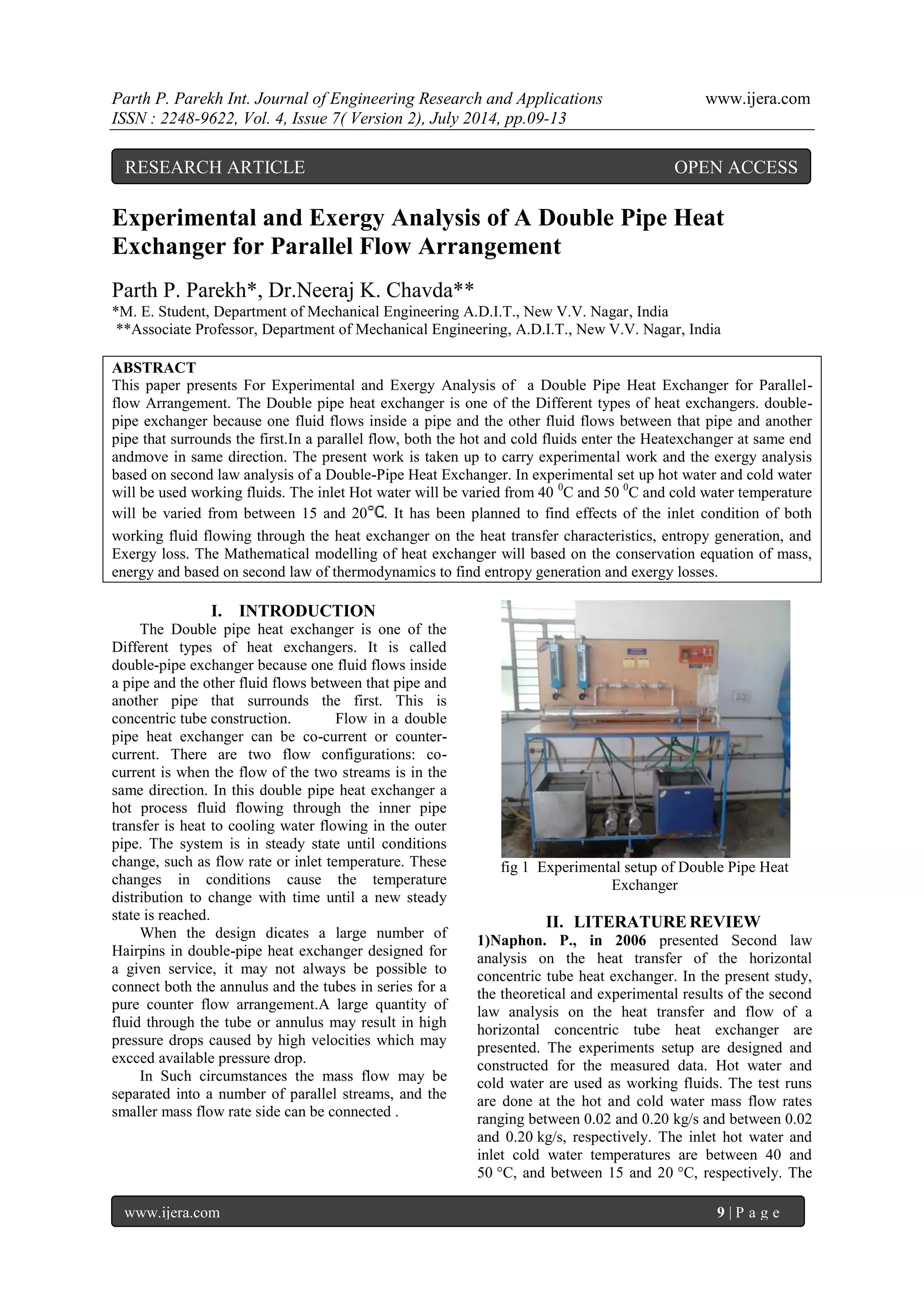
Average Heat Transfer Coefficient Q = 푄퐻+ 푄푐 2 Q =1.3333 KJ/sec Area A= π do L = .1696 m2 ΔT= T4−T1 − T6−T3 ln T4−T1 T6−T3 =18.31 0c Overall heat transfer co-efficient Uo= 푄 퐴×ΔT Uo= 0.2707 W/m2 0c CC = mc Cpc = 0.0.0689 Ch= mh Cph = 0.1368 Ch > Cc Considering case B in [Ref paper no 4 ] Cr = Cmin / Cmax =0.5037 Ɛ= T3−T1 T4−T1 = 0.3937 S! gen=(mcp)h× ln 푇6 푇4 +(mcp)cln 푇3 푇1 =0.0036 W/0c Entropy Generation Number Ns= S!genC min =0.0522 Exergy Loss I!=T0S! gen = 0.1426 Reynold Number For Hot Water at 650c V= 푚푕 휌×퐴푕 퐴푕= 휋 4×D2 퐴푕=1.767×10-4m2 V=0.1887 m/sec Re= 휌×푉×푑 휇 =6394.7126 Pr=2.77 at 650c f=(3.64log Re-3.28)-2 f=0.008945 Nu == (f/2)×(Re−1000)×pr1+12.7× 푓 2 0.5×((pr) 23−1) Nu =36.6042 Nu=hd/k Hhot= Nu×k/d Hhot(Thero)=1618.1497W/m2k QH= Hhot×A×(65-45) Hhot(Practical)=0.2661 W/m2k Reynold Number For Cold Water at 450c Ac=π/4 (Di2-do2) Ac=5.4978×10-4 m2
푉퐶 = 푚푐 휌×퐴푐
푉퐶 =0.0303 m/sec
Pr=4.89 Dc=Di-d0 Dc =0.014m Re= 휌×푉×푑 휇 Re =704.7343 Re ˂ 2300 D/L=4.6667×10-3 Nu =3.657+ 0.0677× Re×pr×DL 1.331+0.1×pr Re×DL 0.33 Nu=4.6562 Nu=hcold×d/k hcold=212.9879 W/m2k Qc=hcold×A×(65-45) hcold(practical)=0.2295 W/m2k [ Table 3 Result Table Case-I]
Sr No
1
2
3
4
5
6
7
8
T1
60.7
62.1
64.1
64.4
57.5
60.4
60.7
58.9
T2
49.9
50.1
49.8
48.9
45.7
46.2
44.3
43.6
푀푕
0.0327
0.0327
0.0326
0.0326
0.0328
0.0327
0.0326
0.0326
푀푐
0.0165
0.0248
0.033
0.0413
0.0496
0.0579
0.0615
0.0744
푄푕
0.9027
1.1899
1.4742
1.9246
1.4937
1.819
2.2385
2.5388
푄푐
0.7786
1.1703
1.5848
1.8282
1.4285
1.7642
1.9253
2.2049
퐻푕표푡(푃푟푎푐)
0.26661
0.3508
0.3477
0.4539
0.44036
0.429
0.4399
0.4989
퐻푕표푡(푡푕푒표)
1618.1497
1618.1497
1684.9024
1684.9024
1543.7251
1618.1497
1684.8712
1684.8712
퐻푐표푙푑(푃푟푎푐)
0.2295
0.345
0.3738
0.4312
0.4211
0.4161
0.3784
0.4333
퐻푐표푙푑(푇푕푒표)
212.9879
284.5708
331.1783
380.5531
376.394
418.3046
634.4367
824.1156
푈0(푃푟푎푐)
0.2707
0.3376
0.38
0.4268
0.4452
0.4597
0.4618
0.5365

4. Parth P. Parekh Int. Journal of Engineering Research and Applications www.ijera.com
ISSN : 2248-9622, Vol. 4, Issue 7( Version 2), July 2014, pp.09-13
www.ijera.com 12 | P a g e
푈0(푇푕푒표)
163.5088
202.6392
226.7111
248.8057
243.112
262.372
336.9715
383.9052
€
0.5113
0.4809
0.2951
0.3507
0.3682
0.3822
0.4069
0.4537
푆푔푒푛
0.0036
0.0087
0.0149
0.0151
0.0109
0.0144
0.015
0. 0177
푁푠
0.0522
0.0839
0.1092
0.1106
0.0737
0.1053
0.1099
0.1297
퐼!
0.1426
0.3445
0.59
0.5979
0.3999
0.5702
0.594
0.7009
Sr No
1
2
3
4
5
6
7
8
T1
52.6
58.3
62.6
66.9
69.5
73.6
75.5
65.7
T2
42.05
44.1
48.7
51.2
53.9
56.8
57.8
52.05
푀푕
0.0164
0.0246
0.0327
0.0407
0.0487
0.0569
0.0648
0.0735
푀푐
0.0331
0.0331
0.0331
0.033
0.033
0.033
0.0329
0.033
푄푕
0.7263
1.1408
1.5181
1.9
1.8587
2.1462
2.3106
1.5986
푄푐
0.6563
0.9257
1.5474
1.8604
2.0006
2.3979
2.5017
1.8122
퐻푕표푡(푃푟푎푐)
0.2855
0.3363
0.358
0.4481
0.3653
0.4218
0.4541
0.3142
퐻푕표푡(푡푕푒표)
676.593
2131.3773
1618.1497
2066.8433
2512.8589
2877.5357
3298.47
3355.9093
퐻푐표푙푑(푃푟푎푐)
0.2579
0.2729
0.3649
0.4388
0.3932
0.4713
0.4917
0.5343
퐻푐표푙푑(푇푕푒표)
296.4418
173.4659
296.4418
331.1783
331.192
331.192
306.3589
331.1783
푈0(푃푟푎푐)
0.2385
0.2781
0.3879
0.4245
0.4443
0.4793
0.4887
0.4668
푈0(푇푕푒표)
171
14
208.
23
239
24
23
24
.6417
2.7142
5906
3.6836
.4561
2.9773
2.1748
6.5319
€
0.4093
0.3469
0.3066
0.3346
0.3699
0.4028
0.4099
0.4109
푆푔푒푛
0.004
0.0049
0.0138
0.0159
0.0181
0.0229
0.023
0.0167
푁푠
0.0584
0.0477
0.1009
0.1154
0.1312
0.1662
0.1673
0.1212
퐼!
0.1584
0.194
0.5465
0.6296
0.7168
0.9068
0.9108
0.6613
[Table 4 Result Table for Parallel Flow(case-II).]
Fig 2 Fig 2 shows that Effectiveness of the case1 is higher to the effectiveness of the case-2.Fig 2 indicate the Effectiveness vs No of Reading.
Fig 3 Fig 3 shows that Entropy generation of case2 is higher to the Entropy generation of the case-1.Fig 3 indicate the Entropy generation vs No of Reading.

5. Parth P. Parekh Int. Journal of Engineering Research and Applications www.ijera.com
ISSN : 2248-9622, Vol. 4, Issue 7( Version 2), July 2014, pp.09-13
www.ijera.com 13 | P a g e
Fig 4 Fig 4 shows that Entropy generation Number of case2 is higher to the Entropy generation Number of the case-1.Fig 4 indicate the Entropy generation Number vs No of Reading. Fig 5shows that Overall Heat Transfer Co- efficient-Practicalof case1 is a Gradually Higher to the Overall Heat Transfer Co-efficient-Practical of the case-2.Fig 5 indicate the Overall Heat Transfer Co-efficient Practical vs No of Reading.
Fig 6 Fig 6 shows that Overall Heat Transfer Co- efficient-Theoraticalof case1 is higher to the Overall Heat Transfer Co-efficient –Theoratical of the case- 2.Fig 6 indicate the Overall Heat Transfer Co- efficient-Theoretical vs No of Reading. Fig 7 shows that Exergy lossof case2 is higher to the of the Exergy lossof case-1.Fig 7 indicate the Exergy loss vs No of Reading.
Fig 7
V. Conclusion
The Second Law analysis on the Heat Transfer of Horizontal Double tube Heat exchanger are presented. The Outcome of the Double Pipe Heat Exchanger for a parallel Arrangement.
 As the const mc and varies mh Effectiveness is higher to the const mh and varies mc
 As the const mh and Varies mc Entropy Generation is higher to const mc and varies mh.
 As the const mh and Varies mc Entropy Generation no is higher to const mc and varies mh.
 As the const mc and varies mh overall heat transfer coefficient practical is higher to the const mh and Varies mc.
 As the const mc and varies mh overall heat transfer coefficient theoretical is higher to the const mh and Varies mc.
 As the const mh and Varies mc Exergy Loss is Higher to the const mc and varies mh.
References
[1] Khairul M.A; Heat transfer performance and exergy analyses of a corrugated plate heat exchanger using metal oxide nano fluids. International Communications in Heat and Mass Transfer.,2013.
[2] Hepbasil. A; Low exergy modelling and performance analysis of greenhouses coupled to closed earth-to-air heat exchangers (EAHEs) ., Energy and Buildings,2013, Volume 64, Pages 224-230.
[3] Qureshi .B .A and Zubair. S.M; Second- law-based performance evaluation of cooling towers and evaporative heat exchangers, International Journal of Thermal Sciences, 2007; Pages 188-198.
[4] Naphon. P.; Second law analysis on the heat transfer of the horizontal concentric tube heat exchanger. International Communications in Heat and Mass Transfer,2006; Pages 1029-1041.
[5] Akpinarn. K. E and Bicer; Investigation of heat transfer and exergy loss in a concentric double pipe exchanger equipped with swirl generators, International Journal of Thermal Sciences,2005, Pages 598-607.