Download as PDF, PPTX


![Brier score
Score-based metrics
When to use it?
● When you care about calibrated probabilities
● Why care about calibration?
y_true = [0, 1, 1, 0, 1, 1, 1, 0]
y_pred_v1 = [0.28, 0.35, 0.32, 0.29, 0.34, 0.38, 0.37, 0.31]
y_pred_v2 = [0.18, 0.95, 0.92, 0.19, 0.94, 0.98, 0.97, 0.21]
1.000, 1.000
0.295, 0.0158
roc_auc_score(y_true, y_pred_v1), roc_auc_score(y_true, y_pred_v2)
brier_score_loss(y_true, y_pred_v1), brier_score_loss(y_true, y_pred_v2)](https://image.slidesharecdn.com/pydatawarsaw122019evaluationmetricsforbinaryclassificationtheultimateguide-191213134324/85/Evaluation-metrics-for-binary-classification-the-ultimate-guide-65-320.jpg)


![Fairness metrics logger
● Log fairness metrics with one function call
● pip install neptune-contrib (link)
● example (link)
Extras
import neptune
import neptunecontrib.monitoring.fairness as npt_fair
neptune.create_experiment()
npt_fair.log_fairness_classification_metrics(
y_true, y_pred, y_class, x_protected,
favorable_label=0, unfavorable_label=1,
privileged_groups={'race':[3]},
unprivileged_groups={'race':[1,2,4]})](https://image.slidesharecdn.com/pydatawarsaw122019evaluationmetricsforbinaryclassificationtheultimateguide-191213134324/85/Evaluation-metrics-for-binary-classification-the-ultimate-guide-81-320.jpg)


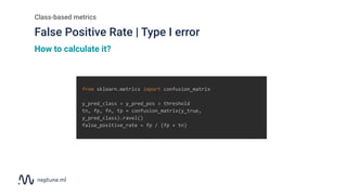
The document is a comprehensive guide on evaluation metrics for binary classification, detailing class-based and score-based metrics along with their applications and calculations. It discusses various statistical measures like confusion matrices, precision, recall, F1 score, ROC curve, and AUC, and provides practical coding examples for implementation. Additionally, it addresses how to choose optimal thresholds and the relevance of different metrics for business problems and model evaluation depending on the dataset characteristics.


![[DL輪読会]FOTS: Fast Oriented Text Spotting with a Unified Network](https://cdn.slidesharecdn.com/ss_thumbnails/20181012yokota-181012004624-thumbnail.jpg?width=640&height=640&fit=bounds)