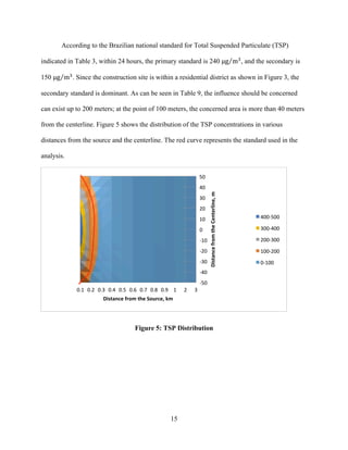
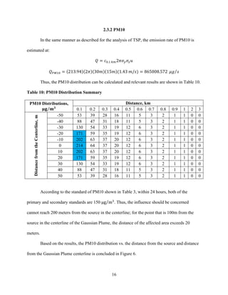
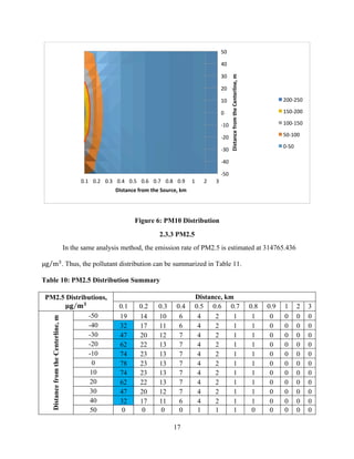
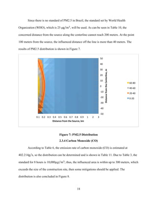
This document provides an analysis of air pollutant distributions from a typical construction site in Brazil. Six major air pollutants are analyzed using the Gaussian plume method. Based on the analysis and air quality standards from Brazil and WHO, emissions of nitrogen dioxide, carbon monoxide, and sulfur dioxide from the construction site pose the highest risk to surrounding areas within 100 meters. Mitigation measures are recommended to control emissions of these pollutants.

![2
In order to understand the impacts on human health, Air Quality Health Index conducted
by Canadian environmental authority is also utilized in the analysis. According to the analysis
results, the risky zone is within the area 100 meters from the emission source.
After the analysis, the mitigating measures are provided. In terms of the mitigations,
controlling the emissions of carbon monoxide, nitrogen dioxide and sulfur dioxide is of
importance since their significant influences. Specifically, since the limitation of resources, the
efficiencies of controlling methods are assumed.
1.2 Problem Statement
As explained in the Session 1.0, with the dramatic growth of the global economy, an
increasing number of construction projects are introduced each year, which leads to the
environmental problems. In the urban area, the emissions of gas pollutants and particulate
matters is of significance; especially for the developing countries, this issue is much more drastic.
Air pollution can cause both acute and chronic effects on public health, impacting on a
large number of different systems and organs. These impacts range from minor upper respiratory
irritation to chronic heart and respiratory disease, lung cancer, acute respiratory infections in
children and chronic bronchitis in adults, aggravating pre-existing heart and lung disease, or
asthmatic attacks. Additionally, short and long-term exposures have also been linked with
reduced life expectancy and premature mortality [1].](https://image.slidesharecdn.com/ffa74084-cfd8-4cb8-a91d-581a6bf0793d-150613000035-lva1-app6892/85/Environmental-Impact-Assessment-Course-Project-2-320.jpg)
![3
1.3 Methodology
This session introduces two methods used in the analysis, namely Gaussian Plume
Method and Air Quality Health Index Method.
1.3.1 Gaussian Plume Method
As introduced above, the gases in analysis can be divided into two categories, namely gas
pollutants and particulate matters. First, the particulate matters include PM 2.5, PM 10, and total
suspended particulates (TSP). The relevant data are obtained from an essay Identification and
Characterization of Particulate Matter Concentration at Construction Jobsites (Araujo, Costa,
and Moraes, 2014). Second, in terms of the gas pollutants, namely sulphur dioxide, carbon
monoxide, and nitrogen dioxide, the emission rates are obtained from a report Building
Assemblies: Construction Energy & Emissions conducted by University of British Columbia in
1993.
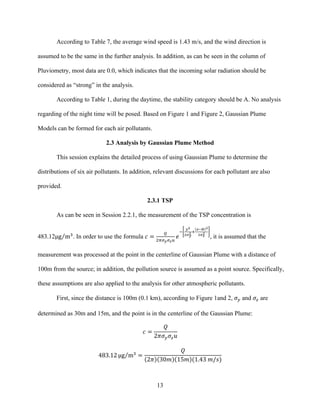
In terms of the analysis method, Gaussian Plume is used to establish the diffusion model.
In the Gaussian Model, it assumes that the air pollutants dispersion has a Gaussian distribution,
which is a normal probability distribution [2]. At present, Gaussian models are usually used to
predict the dispersion of non-continuous air pollution plumes. The basic Gaussian Plume
equation is concluded as:
𝑐 =
𝑄
2𝜋𝜎! 𝜎! 𝑢
𝑒
!
!!
!!!
!!
!!! !
!!!
!
Where:
𝐾! = 0.5𝜎!
!
𝑢
𝑥
𝐾! = 0.5𝜎!
!
𝑢
𝑥
𝑡 =
𝑥
𝑢
𝜎!, 𝜎! = ℎ𝑜𝑟𝑖𝑧𝑜𝑛𝑡𝑎𝑙 𝑎𝑛𝑑 𝑣𝑒𝑟𝑡𝑖𝑐𝑎𝑙 𝑑𝑖𝑠𝑝𝑒𝑟𝑠𝑖𝑜𝑛 𝑐𝑜𝑒𝑓𝑓𝑖𝑐𝑖𝑒𝑛𝑠 (𝑚𝑒𝑡𝑒𝑟)](https://image.slidesharecdn.com/ffa74084-cfd8-4cb8-a91d-581a6bf0793d-150613000035-lva1-app6892/85/Environmental-Impact-Assessment-Course-Project-3-320.jpg)
![4
Horizontal dispersion coefficient 𝜎! can be determined by the diagram shown in Figure 1,
and Figure 2 demonstrates the relationship between the downwind distance and vertical
dispersion coefficient 𝜎!. [3]
Specifically, since the construction site is close to the residential district with low-rise
buildings, only the air near the ground will be analyzed, which means “z-H” in the formula
should be 0.
Figure 1: Horizontal Dispersion Coefficient 𝝈 𝒚 as a Function of Downwind Distance from
the Source for Various Stability Categories.](https://image.slidesharecdn.com/ffa74084-cfd8-4cb8-a91d-581a6bf0793d-150613000035-lva1-app6892/85/Environmental-Impact-Assessment-Course-Project-4-320.jpg)
![5
Figure 2: Vertical Dispersion Coefficient 𝝈 𝒛as a Function of Downwind Distance from the
Source for Various Stability Categories
In terms of the stability categories, Table 1 introduces the relevant information.
Table 1: Key to Stability Categories [4]](https://image.slidesharecdn.com/ffa74084-cfd8-4cb8-a91d-581a6bf0793d-150613000035-lva1-app6892/85/Environmental-Impact-Assessment-Course-Project-5-320.jpg)
![6
1.3.2 Air Quality Health Index
The Air Quality Health Index (AQHI) is a public information tool used in Canada to
prevent people’s health from the negative effects of air pollution on a daily basis. Basically, it is
measured by the formula:
𝐴𝑄𝐻𝐼 =
100
10.4
× 𝑒!.!!!"#$×!!! − 1 + 𝑒!.!!!"#$×!!"! − 1 + 𝑒!.!!!"#$×!!"!.! − 1
Where:
𝑐!!
= Concentration of ozone, ppb
𝑐!"!
= Concentration of NO2, ppb
𝑐!"!.! = Concentration of PM2.5, 𝜇𝑔 𝑚!
After obtaining the value of Air Quality Health Index, the influence level can be
determined by Table 2.
Table 2: Canadian Air Quality Health Index Reference Table [5]
Specifically, in this report, only the points along the centerline of the Gaussian Plume are
analyzed by AQHI because the values along the centerline should be the most critical.](https://image.slidesharecdn.com/ffa74084-cfd8-4cb8-a91d-581a6bf0793d-150613000035-lva1-app6892/85/Environmental-Impact-Assessment-Course-Project-6-320.jpg)
![7
1.4 Construction Site Introduction
The studied construction site is located in Salvador, Bahia, Brazil, (latitude 12°57’46”
south, longitude 38°24’32” west) at an altitude of 34 m. The proposed project contains 8
residential towers, each with 16 floors, totaling 464 housing units. The total construction area is
32,780 m2
. [6] Figure 3 introduces the construction location obtained by Google Earth.
Specifically, since there is no explanation of the dimensions of construction site, the area is
assumed to be a square, and the length of each side is 181 m.
The construction site is located in a low-rise residential district with the appearance of
flora and fauna, including a lake. Within an area of 100 m, there is no primary pollution source
such as other construction sites, industries, major highways and airports. [7]
Figure 3: Construction Site (via Google Earth)
A typical series of construction activities for reinforced concrete structures can be
categorized into 3 major phases, namely the earthwork, superstructure, and finishing. First, the
earthwork includes manual excavation, meso structure, razing of auger piles foundation,
vehicular traffic on the soil, land transportation, and truck traffic at the construction site. Second,](https://image.slidesharecdn.com/ffa74084-cfd8-4cb8-a91d-581a6bf0793d-150613000035-lva1-app6892/85/Environmental-Impact-Assessment-Course-Project-7-320.jpg)
![9
2.0 CASE STUDY
This session introduces the air quality standards posed by Brazilian relevant authorities
and World Health Organization, the means of data collections, and the analysis of atmospheric
pollutants by Gaussian Plume Method.
2.1 Air Quality Standards
In Brazil, the standardized pollutants are TSP, smoke, sulfur dioxide (SO2), inhalable
particles, carbon monoxide (CO), and nitrogen dioxide (NO2). The Brazilian National
Environmental Council (CONAMA) Resolution Number 3 published on August 1990 indicates
that the primary standards should be adopted if relevant area classes are not established [8].
Table 3: Brazilian National Air Quality Standards [9]
Pollutant Averaging Time Primary Standards Secondary Standards
TSP 24 h 240 𝜇𝑔 𝑚!
150 𝜇𝑔 𝑚!
Geometric Annual Average 80 𝜇𝑔 𝑚!
60 𝜇𝑔 𝑚!
PM10 24 h 150 𝜇𝑔 𝑚!
Arithmetic Annual Average 50 𝜇𝑔 𝑚!
SO2 24 h 365 𝜇𝑔 𝑚!
100 𝜇𝑔 𝑚!
Arithmetic Annual Average 80 𝜇𝑔 𝑚!
40 𝜇𝑔 𝑚!
CO 1 h 40,000 𝜇𝑔 𝑚!
8 h 10,000 𝜇𝑔 𝑚!
NO2 1 h 320 𝜇𝑔 𝑚!
190 𝜇𝑔 𝑚!
Arithmetic Annual Average 100 𝜇𝑔 𝑚!
Since there is no standard of PM2.5 in Brazil, the standard posted by World Health
Organization (WHO) will be used in this report. Thus, the PM2.5 concentration should be 25
µμg m!
within 24 hours, and 10 µμg m!
within a year.](https://image.slidesharecdn.com/ffa74084-cfd8-4cb8-a91d-581a6bf0793d-150613000035-lva1-app6892/85/Environmental-Impact-Assessment-Course-Project-9-320.jpg)
![10
2.2 Data
This session explains the means of data collections, the specific numbers will be used for
further analysis in Session 2.3, and the situation of the meteorology.
2.2.1 Particulate matters
As introduced previously, the particulate matters include PM 2.5, PM 10, and Total
Suspended Particulates (TSP). According to the essay Identification and Characterization of
Particulate Matter Concentration at Construction Jobsites, the concentrations of these three
pollutants were obtained by the MiniVols Equipment because of it portability (the appearance is
shown in Figure 4). It was installed during three major construction phases, namely earthworks,
superstructure, and finishing; for each phase, the detection period was 10 days.
Figure 4: MiniVols [10]
In order to decrease the influence from the existed particulate matters in the air, there
were two sets of equipment were installed. One set was placed at the construction site entrance
for measuring the concentrations of PMs entering the construction site, and the other set was
installed at the end of the construction site for measuring the PMs exiting the construction site.
The measuring operations were performed at the same periods. The measuring period is
introduced in Table 4.](https://image.slidesharecdn.com/ffa74084-cfd8-4cb8-a91d-581a6bf0793d-150613000035-lva1-app6892/85/Environmental-Impact-Assessment-Course-Project-10-320.jpg)
![11
Table 4: Measuring Schedule [11]
Shifts Schedule Period Length
Day 7 am to 3 pm 8 hours
Night 5 pm to 3 pm 22 hours
After adjusting the measurements by subtracting the PMs existing the air, the PMs
produced during the construction are shown in Table 5 [12].
Table 5: Descriptive Statistics of PM Concentrations in 𝝁𝒈 𝒎 𝟑
for Three Construction
Phases
As can be seen in Table 5, all the maximum average concentrations of three studied
particulate matters occurred during the Phase 2 that is superstructure. Results are 483.12 µμg m!
for TSP, 213.94 µμg m!
for PM10, and 77.85 µμg m!
for PM2.5. These results will be discussed
in later sessions.
2.2.2 Gas Pollutants
In terms of the gas pollutants, according to the report Building Assemblies: Construction
Energy & Emissions conducted by University of British Columbia in 1993, the maximum
emissions of three major gas pollutants are introduced in Table 6.
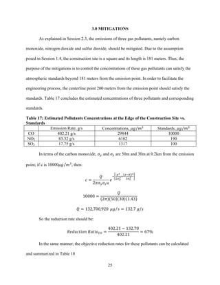
Table 6: Maximum Emissions of Three Major Gas pollutants [13]
Gas pollutants Maximum Emissions
CO 402.21 g/s
NOx 83.32 g/s
SO2 17.75 g/s](https://image.slidesharecdn.com/ffa74084-cfd8-4cb8-a91d-581a6bf0793d-150613000035-lva1-app6892/85/Environmental-Impact-Assessment-Course-Project-11-320.jpg)
![12
In the further study, the concentration of nitrogen gas pollutants (NOx) is regarded as the
nitrogen dioxide (NO2).
2.2.3 Meteorology
During measuring the concentrations of particulate matters, the meteorological data were
also recorded and concluded in the essay Identification and Characterization of Particulate
Matter Concentration at Construction Jobsites (Araujo, Costa, and Moraes, 2014). Table 7
shows the relevant data.
Table 7: Meteorological Data during Measuring [14]](https://image.slidesharecdn.com/ffa74084-cfd8-4cb8-a91d-581a6bf0793d-150613000035-lva1-app6892/85/Environmental-Impact-Assessment-Course-Project-12-320.jpg)
![23
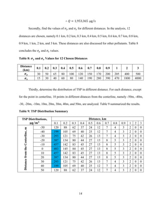
2.4 Analysis by Air Quality Health Index
According to the analysis by the Gaussian Plume, the concentrations of Nitrogen Dioxide
and PM2.5 along the centerline of the Gaussian Plume are determined. In terms of the ozone,
Table 14 shows the ozone level measured in a construction site.
Table 14: Ozone Produced During Construction [15]
The 0.12ppm is chosen as the estimated concentration of ozone in a typical construction
site. Use the same way explained in Session 2.3.1 to determine the emission rate of ozone, then
determine the distribution along the Gaussian Plume centerline. The concentrations of three
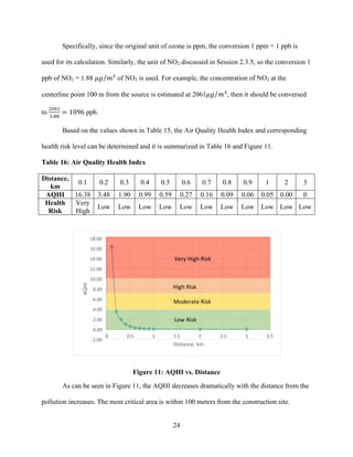
major elements in the AQHI formula are shown in Table 15.
Table 15: Concentrations of Ozone, Nitrogen Dioxide and PM2.5 along Centerline
Distance,
km
0.1 0.2 0.3 0.4 0.5 0.6 0.7 0.8 0.9 1 2 3
Ozone,
ppb
120 36 21 11 7 3 2 1 1 1 0 0
NO2,
ppb
1096 329 190 103 62 29 18 10 6 5 1 0
PM2.5,
𝝁𝒈 𝒎 𝟑 78 23 13 7 4 2 1 1 0 0 0 0](https://image.slidesharecdn.com/ffa74084-cfd8-4cb8-a91d-581a6bf0793d-150613000035-lva1-app6892/85/Environmental-Impact-Assessment-Course-Project-23-320.jpg)
![26
Table 18: Objectives of Reduction Rates
Objective Reduction Rates
CO 67%
NO2 97%
SO2 93%
In order to achieve these objectives, here are some specific measures based on the
guideline Air Pollution Control at Construction Sites posed by Swiss Agency for the
Environment, Forests and Landscape (SAEFL) (2004).
Table 19: Mitigating Measures [16]
Construction
Activities
Mitigations
ThermalandChemicalWork
Processes
Restrict the thermal preparation of tar-based material and coating at building
sites
Use the asphalt or bitumen that has low emission rates of air pollutants
Use bitumen emulsions instead of bitumen solutions
Apply appropriate measures for binding material to lower the processing
temperature
In order to abate the welding emissions, it is necessary to capture, extract (e.g.
spot suction) and filter the emitted fumes.
When treat the surface or glue/seal the gaps, choose eco-friendly products
Deploy low emission explosives (e.g. formulated as emulsion, slurry or water
gel)
Stipulationsfor
MachinesAnd
Equipment
Use low-emission equipment (e.g. powered with electrical motors)
Equip and maintain combustion-engine powered tools/machines based on the
manufacturers’ specifications
Use low-sulfur fuels (sulfur content <50ppm) for machines and equipment to
power the diesel engines
Diesel-powered machines and equipment must be equipped with particle trap
systems (PTS) or other equivalently effective emission curtailment traps
Construction
Fulfillment
For scheduling, the contractor must submit the pertinent list before work
begins, and regularly update the list in order to ensure punctual availability of
the appropriate machines and equipment (a sample of pertinent list is shown
in Appendix A)
Train the workers about the origin, dispersal, impact and abatement of
airborne pollutants in order to promote the relevant awareness](https://image.slidesharecdn.com/ffa74084-cfd8-4cb8-a91d-581a6bf0793d-150613000035-lva1-app6892/85/Environmental-Impact-Assessment-Course-Project-26-320.jpg)
![29
REFERENCE
[1] ‘Spare The Air: Health Effects of Air Pollution’, Air Quality Information for the Sacramento
Region. [Online]. Available: http://www.sparetheair.com/health.cfm?page=healthoverall.
[Accessed: 10-Apr-2015].
[2] M. R. Beychok, Fundamentals of stack gas dispersion, 4th ed. Irvine, CA: Milton R.
Beychok, 1994.
[3] N. De Nevers, Air Pollution Control Engineering. William C Brown Pub, 2000.
[4] N. De Nevers, Air Pollution Control Engineering. William C Brown Pub, 2000.
[5] ‘Air Quality Health Index - Home - Air - Environment Canada’, Environment Canada.
[Online]. Available: https://ec.gc.ca/cas-aqhi/default.asp?lang=En. [Accessed: 10-Apr-2015].
[6] I. P. S. Araujo, D. B. Costa, and R. J. B. de Moraes, ‘Identification and Characterization of
Particulate Matter Concentrations at Construction Jobsites’, Nov. 2014.
[7] I. P. S. Araujo, D. B. Costa, and R. J. B. de Moraes, ‘Identification and Characterization of
Particulate Matter Concentrations at Construction Jobsites’, Nov. 2014.
[8] I. P. S. Araujo, D. B. Costa, and R. J. B. de Moraes, ‘Identification and Characterization of
Particulate Matter Concentrations at Construction Jobsites’, Nov. 2014.
[9] ‘Brazil: Air Quality Standards’, Tansportpolicy.net, 07-May-2014. [Online]. Available:
http://transportpolicy.net/index.php?title=Brazil:_Air_Quality_Standards. [Accessed: 03-Apr-
2015].
[10] I. P. S. Araujo, D. B. Costa, and R. J. B. de Moraes, ‘Identification and Characterization of
Particulate Matter Concentrations at Construction Jobsites’, Nov. 2014.](https://image.slidesharecdn.com/ffa74084-cfd8-4cb8-a91d-581a6bf0793d-150613000035-lva1-app6892/85/Environmental-Impact-Assessment-Course-Project-29-320.jpg)
![30
[11] I. P. S. Araujo, D. B. Costa, and R. J. B. de Moraes, ‘Identification and Characterization of
Particulate Matter Concentrations at Construction Jobsites’, Nov. 2014.
[12] I. P. S. Araujo, D. B. Costa, and R. J. B. de Moraes, ‘Identification and Characterization of
Particulate Matter Concentrations at Construction Jobsites’, Nov. 2014.
[13] The Environmental Research Group, Building Assemblies: Construction Energy &
Emissions. Vancouver: University of British Columbia, 1993.
[14] I. P. S. Araujo, D. B. Costa, and R. J. B. de Moraes, ‘Identification and Characterization of
Particulate Matter Concentrations at Construction Jobsites’, Nov. 2014.
[15] Hazard Evaluation and Technical Assistance Branch of NIOSH, ‘Ozone Exposure at a
Construction Site’, Apr. 1999.
[16] A. Staubli and R. Kropf, Air Pollution Control at Construction Sites. Berne: Swiss Agency
for the Environment, Forests and Landscape, 2004.](https://image.slidesharecdn.com/ffa74084-cfd8-4cb8-a91d-581a6bf0793d-150613000035-lva1-app6892/85/Environmental-Impact-Assessment-Course-Project-30-320.jpg)


