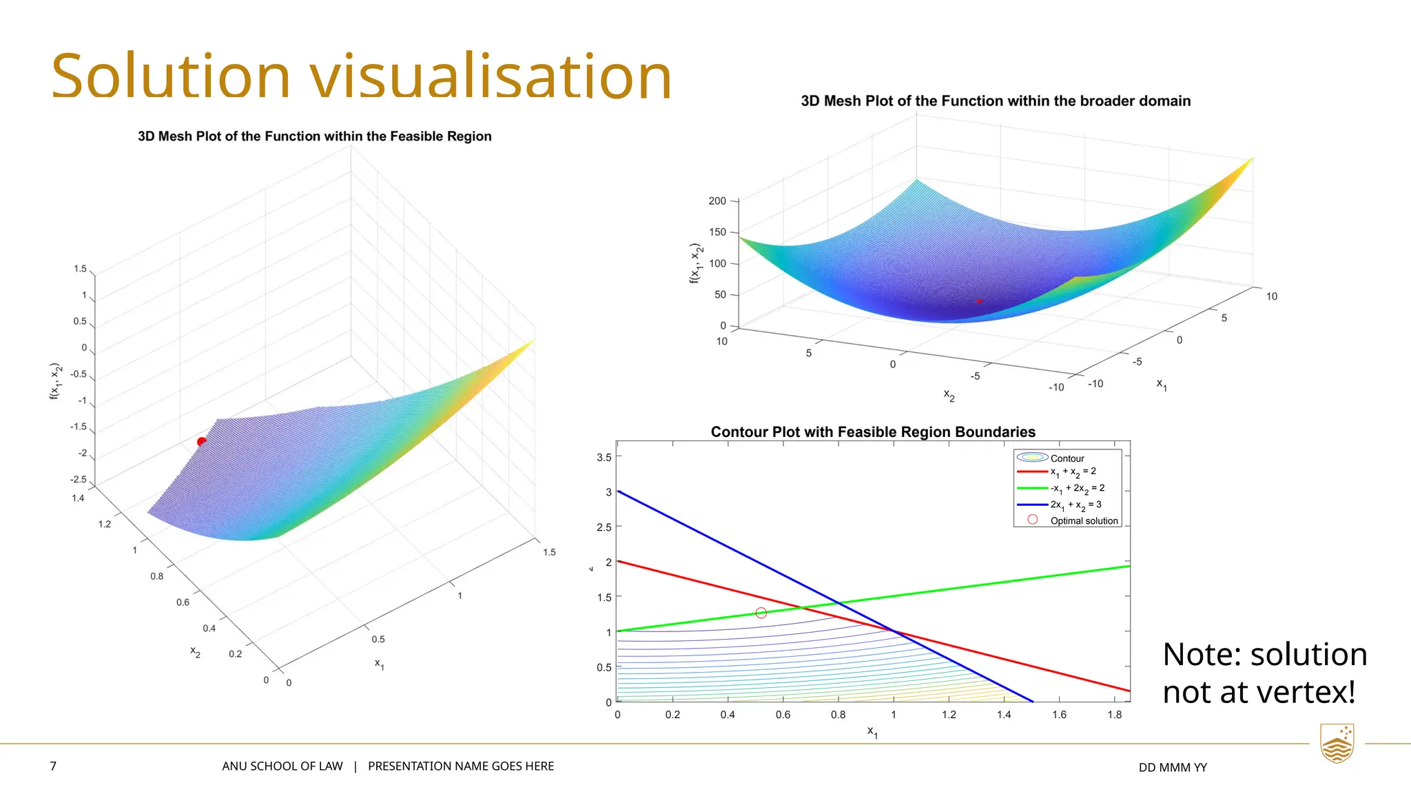
ENGN3301
OPERATIONS RESEARCH
NONLINEAR PROGRAMMING
QUADRATIC PROGRAMING
2 ANU SCHOOL OF ENGINEERING | EB4 QUADRATIC PROGRAMMING
Linear Programming (LP)
• Recall the anatomy of a linear program
• Decision variables: (with lower and upper bounds)
• Objective function (linear): (minimise/maximise)
• Constraints: (inequality, equality)
In matrix form (Matlab-preferred formulation):
For a LP problem, the optimal solution is always at
one of the vertices of the feasibility region.
Objective function: a plane in space
(for a problem with 2 decision variables)
“house with a flat roof”
3
Non-Linear
Programming
ANU SCHOOL OF ENGINEERING | EB4 QUADRATIC PROGRAMMING
• Objective function:
Minimise:
• Constraints:
• If the function or one of the
constraints or is non-linear, that is a
case of
non-linear programming.
• The optimal solution is no longer
guaranteed to be at the feasibility
region boundary / vertex
• Quadratic Programming is a special
case of non-linear programming
A nonlinear objective function, also plotted as contours
superimposed on the feasibility region
4 ANU SCHOOL OF ENGINEERING | EB4 QUADRATIC PROGRAMMING
Quadratic Programming (QP)
• Objective function has degree 2, e.g.,
• All the constraints and are linear (same as LP)
• Any QP can be defined as:
Such
that:
: number of decision variables
: number of equality constraints
: number of inequality constraints
min
𝑥
1
2
𝑥
𝑇
𝐻𝑥+ 𝑓
𝑇
𝑥
𝑧=𝑥1
2
+2 𝑥1 𝑥2+3 𝑥2
DD MMM YY
• Investment decisions across
collection of financial assets
(eg. stocks)
• Machine learning: Least
squares
• Satellite Slew Control
• Minimising manufacturing
cost (problems with
economies/diseconomies of
scale)
• Many other problems with
quadratic formulation.
5
Applications of
QPs
Photo
by
Callum
Wale
on
Unsplash
ANU SCHOOL OF ENGINEERING | EB4 QUADRATIC PROGRAMMING
6
Matlab solution of Quadratic Problem
ANU SCHOOL OF ENGINEERING | EB4 QUADRATIC PROGRAMMING
• Minimize:
• Such that:

• Bounds
H = 2*[1/2 -1/8;
-1/8 1]; %H matrix standard form
f = [0.1; -3]; % same for f
A = [1 1;
-1 2;
2 1];
b = [2; 2; 3];
lb = zeros(2,1);
ub = [10, 10];
Aeq = [];
beq = [];
[x,fval] = quadprog(H,f,A,b,Aeq,beq,lb,ub);
x = [0.5200 1.2600] // optimal solution
𝐦𝐢𝐧
𝒙
𝟏
𝟐
𝒙
𝑻
𝑯𝒙 + 𝒇
𝑻
𝒙
ANU SCHOOL OF LAW | PRESENTATION NAME GOES HERE
7 DD MMM YY
Solution visualisation
Contour Plot with Feasible Region Boundaries
0 0.2 0.4 0.6 0.8 1 1.2 1.4 1.6 1.8
x1
0
0.5
1
1.5
2
2.5
3
3.5
x
2
Contour
x1
+ x2
= 2
-x1
+ 2x2
= 2
2x1
+ x2
= 3
Optimal solution
Note: solution
not at vertex!
ANU SCHOOL OF LAW | PRESENTATION NAME GOES HERE
8 DD MMM YY
Equation to matrix form for solution
𝐦𝐢𝐧
𝒙
𝟏
𝟐
𝒙
𝑻
𝑯𝒙 + 𝒇
𝑻
𝒙
𝑧 =
1
2
𝑥1
2
+ 𝑥2
2
−
1
4
𝑥1 𝑥2 +
1
10
𝑥1 − 3 𝑥2
H = 2*[1/2 -1/8;
-1/8 1];
half of
coefficient
coefficient
for
coefficient
for
2x scaling factor as
the Matlab formulation
expects a ½ fraction in front
f = [0.1; -3];
half of
coefficient
(symmetric matrix)
coefficients for
DD MMM YY
1. Interior Point
2. Active set
3. Augmented Lagrangian
4. Conjugate gradient
5. Gradient Projection
Various methods depending on nature of
the problem (e.g., dense vs sparse H),
precision vs speed trade-offs etc.
9
Different methods
to solve QP
Photo
by
Viswanath
V
Pai
on
Unsplash
ANU SCHOOL OF ENGINEERING | EB4 QUADRATIC PROGRAMMING
ANU SCHOOL OF LAW | PRESENTATION NAME GOES HERE
10
Assume two warehouses and two stores, with transport between them.
DD MMM YY
Example: transport with congestion
𝑥1
𝑥2
𝑥3
𝑥4
THANK YOU

ENGN3301_Quadratic_Programming_2024.pptx

  • 1.
  • 2.
    2 ANU SCHOOLOF ENGINEERING | EB4 QUADRATIC PROGRAMMING Linear Programming (LP) • Recall the anatomy of a linear program • Decision variables: (with lower and upper bounds) • Objective function (linear): (minimise/maximise) • Constraints: (inequality, equality) In matrix form (Matlab-preferred formulation): For a LP problem, the optimal solution is always at one of the vertices of the feasibility region. Objective function: a plane in space (for a problem with 2 decision variables) “house with a flat roof”
  • 3.
    3 Non-Linear Programming ANU SCHOOL OFENGINEERING | EB4 QUADRATIC PROGRAMMING • Objective function: Minimise: • Constraints: • If the function or one of the constraints or is non-linear, that is a case of non-linear programming. • The optimal solution is no longer guaranteed to be at the feasibility region boundary / vertex • Quadratic Programming is a special case of non-linear programming A nonlinear objective function, also plotted as contours superimposed on the feasibility region
  • 4.
    4 ANU SCHOOLOF ENGINEERING | EB4 QUADRATIC PROGRAMMING Quadratic Programming (QP) • Objective function has degree 2, e.g., • All the constraints and are linear (same as LP) • Any QP can be defined as: Such that: : number of decision variables : number of equality constraints : number of inequality constraints min 𝑥 1 2 𝑥 𝑇 𝐻𝑥+ 𝑓 𝑇 𝑥 𝑧=𝑥1 2 +2 𝑥1 𝑥2+3 𝑥2
  • 5.
    DD MMM YY •Investment decisions across collection of financial assets (eg. stocks) • Machine learning: Least squares • Satellite Slew Control • Minimising manufacturing cost (problems with economies/diseconomies of scale) • Many other problems with quadratic formulation. 5 Applications of QPs Photo by Callum Wale on Unsplash ANU SCHOOL OF ENGINEERING | EB4 QUADRATIC PROGRAMMING
  • 6.
    6 Matlab solution ofQuadratic Problem ANU SCHOOL OF ENGINEERING | EB4 QUADRATIC PROGRAMMING • Minimize: • Such that:  • Bounds H = 2*[1/2 -1/8; -1/8 1]; %H matrix standard form f = [0.1; -3]; % same for f A = [1 1; -1 2; 2 1]; b = [2; 2; 3]; lb = zeros(2,1); ub = [10, 10]; Aeq = []; beq = []; [x,fval] = quadprog(H,f,A,b,Aeq,beq,lb,ub); x = [0.5200 1.2600] // optimal solution 𝐦𝐢𝐧 𝒙 𝟏 𝟐 𝒙 𝑻 𝑯𝒙 + 𝒇 𝑻 𝒙
  • 7.
    ANU SCHOOL OFLAW | PRESENTATION NAME GOES HERE 7 DD MMM YY Solution visualisation Contour Plot with Feasible Region Boundaries 0 0.2 0.4 0.6 0.8 1 1.2 1.4 1.6 1.8 x1 0 0.5 1 1.5 2 2.5 3 3.5 x 2 Contour x1 + x2 = 2 -x1 + 2x2 = 2 2x1 + x2 = 3 Optimal solution Note: solution not at vertex!
  • 8.
    ANU SCHOOL OFLAW | PRESENTATION NAME GOES HERE 8 DD MMM YY Equation to matrix form for solution 𝐦𝐢𝐧 𝒙 𝟏 𝟐 𝒙 𝑻 𝑯𝒙 + 𝒇 𝑻 𝒙 𝑧 = 1 2 𝑥1 2 + 𝑥2 2 − 1 4 𝑥1 𝑥2 + 1 10 𝑥1 − 3 𝑥2 H = 2*[1/2 -1/8; -1/8 1]; half of coefficient coefficient for coefficient for 2x scaling factor as the Matlab formulation expects a ½ fraction in front f = [0.1; -3]; half of coefficient (symmetric matrix) coefficients for
  • 9.
    DD MMM YY 1.Interior Point 2. Active set 3. Augmented Lagrangian 4. Conjugate gradient 5. Gradient Projection Various methods depending on nature of the problem (e.g., dense vs sparse H), precision vs speed trade-offs etc. 9 Different methods to solve QP Photo by Viswanath V Pai on Unsplash ANU SCHOOL OF ENGINEERING | EB4 QUADRATIC PROGRAMMING
  • 10.
    ANU SCHOOL OFLAW | PRESENTATION NAME GOES HERE 10 Assume two warehouses and two stores, with transport between them. DD MMM YY Example: transport with congestion 𝑥1 𝑥2 𝑥3 𝑥4
  • 11.