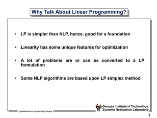
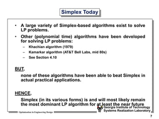
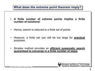
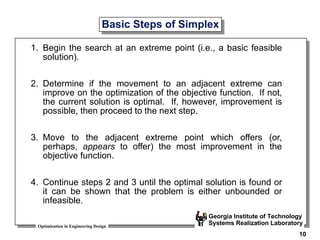
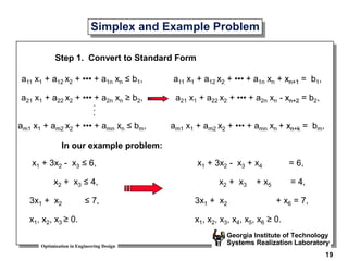
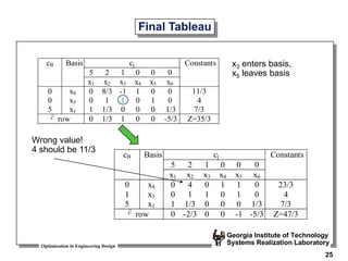
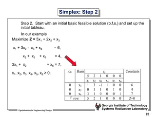
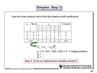
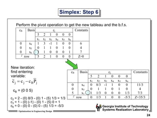
The document discusses linear programming (LP) and the simplex method for solving LP problems. It provides the following key points: - LP is simpler than nonlinear programming and many problems can be formulated as LP problems. - The simplex method provides an efficient systematic approach to solve LP problems by moving between extreme points in finite steps. - The simplex method works by starting at an initial basic feasible solution and iteratively moving to adjacent extreme points to optimize the objective function, until an optimal solution is found. 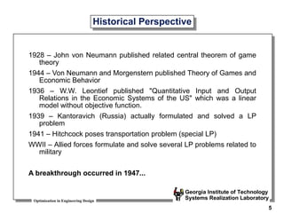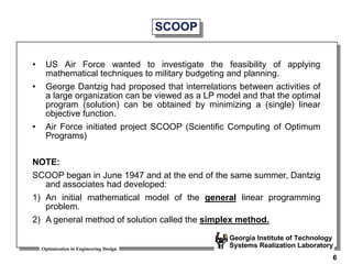- George Dantzig developed the simplex method in 1947 to solve military planning problems, establishing it as the most commonly used algorithm for solving LP problems.

1. Optimization in Engineering Design
Georgia Institute of Technology
Systems Realization Laboratory
1
Linear Programming (LP)

2. Optimization in Engineering Design
Georgia Institute of Technology
Systems Realization Laboratory
2
Why Talk About Linear Programming?
• LP is simpler than NLP, hence, good for a foundation
• Linearity has some unique features for optimization
• A lot of problems are or can be converted to a LP
formulation
• Some NLP algorithms are based upon LP simplex method

3. Optimization in Engineering Design
Georgia Institute of Technology
Systems Realization Laboratory
3
Bolted Joint Design
Given
At - tensile strength area, function of d
Db - bolt circle diameter
Pt - total load
C - joint constant
Fi - preload (= 0.75 Sp At)
Find
N - number of bolts, Sp - proof strength, d - diameter
Satisfy
3d   Db / N good wrench rule
 Db / N  6d good seal rule
C Pt / N  Sp At - Fi static loading constraint
Fi  (1 - C) Pt / N joint separation constraint
Minimize Z= [ f1(N, d, Sp), f2(N, d, Sp), ..]
Question:
Is this a linear or
nonlinear model?

4. Optimization in Engineering Design
Georgia Institute of Technology
Systems Realization Laboratory
4
Bolted Joint Design (2)
Given
d - diameter
At - tensile strength area, function of d
Db - bolt circle diameter
Pt - total load
C - joint constant
Fi - preload (= 0.75 Sp At)
Find
N - number of bolts, Sp - proof strength
Satisfy
3d   Db / N good wrench rule
 Db / N  6d good seal rule
C Pt / N  Sp At - Fi static loading constraint
Fi  (1 - C) Pt / N joint separation constraint
Minimize Z= [ f1(N, Sp), f2(N, Sp), ..]
Question:
Is this a linear or
nonlinear problem?

5. Optimization in Engineering Design
Georgia Institute of Technology
Systems Realization Laboratory
5
Historical Perspective
1928 – John von Neumann published related central theorem of game
theory
1944 – Von Neumann and Morgenstern published Theory of Games and
Economic Behavior
1936 – W.W. Leontief published "Quantitative Input and Output
Relations in the Economic Systems of the US" which was a linear
model without objective function.
1939 – Kantoravich (Russia) actually formulated and solved a LP
problem
1941 – Hitchcock poses transportation problem (special LP)
WWII – Allied forces formulate and solve several LP problems related to
military
A breakthrough occurred in 1947...

6. Optimization in Engineering Design
Georgia Institute of Technology
Systems Realization Laboratory
6
SCOOP
• US Air Force wanted to investigate the feasibility of applying
mathematical techniques to military budgeting and planning.
• George Dantzig had proposed that interrelations between activities of
a large organization can be viewed as a LP model and that the optimal
program (solution) can be obtained by minimizing a (single) linear
objective function.
• Air Force initiated project SCOOP (Scientific Computing of Optimum
Programs)
NOTE:
SCOOP began in June 1947 and at the end of the same summer, Dantzig
and associates had developed:
1) An initial mathematical model of the general linear programming
problem.
2) A general method of solution called the simplex method.

7. Optimization in Engineering Design
Georgia Institute of Technology
Systems Realization Laboratory
7
Simplex Today
• A large variety of Simplex-based algorithms exist to solve
LP problems.
• Other (polynomial time) algorithms have been developed
for solving LP problems:
– Khachian algorithm (1979)
– Kamarkar algorithm (AT&T Bell Labs, mid 80s)
– See Section 4.10
BUT,
none of these algorithms have been able to beat Simplex in
actual practical applications.
HENCE,
Simplex (in its various forms) is and will most likely remain
the most dominant LP algorithm for at least the near future

8. Optimization in Engineering Design
Georgia Institute of Technology
Systems Realization Laboratory
8
Fundamental Theorem
Extreme point (or Simplex filter) theorem:
If the maximum or minimum value of a
linear function defined over a polygonal
convex region exists, then it is to be found
at the boundary of the region.
Convex set:
A set (or region) is convex if, for any two points (say, x1
and x2) in that set, the line segment joining these points
lies entirely within the set.
A point is by definition convex.

9. Optimization in Engineering Design
Georgia Institute of Technology
Systems Realization Laboratory
9
What does the extreme point theorem imply?
• A finite number of extreme points implies a finite
number of solutions!
• Hence, search is reduced to a finite set of points
• However, a finite set can still be too large for practical
purposes
• Simplex method provides an efficient systematic search
guaranteed to converge in a finite number of steps.

10. Optimization in Engineering Design
Georgia Institute of Technology
Systems Realization Laboratory
10
Basic Steps of Simplex
1. Begin the search at an extreme point (i.e., a basic feasible
solution).
2. Determine if the movement to an adjacent extreme can
improve on the optimization of the objective function. If not,
the current solution is optimal. If, however, improvement is
possible, then proceed to the next step.
3. Move to the adjacent extreme point which offers (or,
perhaps, appears to offer) the most improvement in the
objective function.
4. Continue steps 2 and 3 until the optimal solution is found or
it can be shown that the problem is either unbounded or
infeasible.

11. Optimization in Engineering Design
Georgia Institute of Technology
Systems Realization Laboratory
11
Step 0 – Obtain Canonical Form
General Simplex LP model:
min (or max) z =  ci xi
s.t.
A x = b
x  0
In order to get and maintain this form, use
• slack, if x  b, then x + slack = b
• surplus, if x  b, then x - surplus = b
• artificial variables (sometimes need to be added to ensure all
variables  0, see page 101)
Compare constraint conversion with goal
conversions using deviation variables
IMPORTANT: Simplex only deals with equalities

12. Optimization in Engineering Design
Georgia Institute of Technology
Systems Realization Laboratory
12
Different "components" of a LP model
• LP model can always be split into a basic and a non-
basic part.
• “Transformed” or “reduced” model is another good way
to show this.
• This can be represented in mathematical terms as well
as in a LP or simplex tableau.

13. Optimization in Engineering Design
Georgia Institute of Technology
Systems Realization Laboratory
13
Movement to Adjacent Extreme Point
Given any basis we move to an adjacent extreme point
(another basic feasible solution) of the solution space by
exchanging one of the columns that is in the basis for a
column that is not in the basis.
Two things to determine:
1) which (nonbasic) column of A should be brought into
the basis so that the solution improves?
2) which column can be removed from the basis such that
the solution stays feasible?

14. Optimization in Engineering Design
Georgia Institute of Technology
Systems Realization Laboratory
14
Entering and Departing Vector (Variable) Rules
General rules:
• The one non-basic variable to come in is the one which
provides the highest reduction in the objective function.
• The one basic variable to leave is the one which is
expected to go infeasible first.
NOTE: THESE ARE HEURISTICS!!
Variations on these rules exist, but are rare.

15. Optimization in Engineering Design
Georgia Institute of Technology
Systems Realization Laboratory
15
Simplex Variations
Various variations on the simplex method exist:
• "regular" simplex (see Section 4.4)
• two-phase method: Phase I for feasibility and Phase II
for optimality (see Section 4.5.1)
• condensed/reduced/revised method: only use the non-
basic columns to work with (see Section 4.6)
• (revised) dual simplex (see Section 4.8), etc.

16. Optimization in Engineering Design
Georgia Institute of Technology
Systems Realization Laboratory
16
Computational Considerations
• Unrestricted variables (unboundedness)
• Redundancy (linear dependency, modeling errors)
• Degeneracy (some basic variables = 0)
• Round-off errors

17. Optimization in Engineering Design
Georgia Institute of Technology
Systems Realization Laboratory
17
Limitations of Simplex
1. Inability to deal with multiple objectives
2. Inability to handle problems with integer variables
Problem 1 is solved using Multiplex
Problem 2 has resulted in:
• Cutting plane algorithms (Gomory, 1958)
• Branch and Bound (Land and Doig, 1960)
However,
solution methods to LP problems with integer or Boolean
variables are still far less efficient than those which include
continuous variables only

18. Optimization in Engineering Design
Georgia Institute of Technology
Systems Realization Laboratory
18
Example Problem
Maximize Z = 5x1 + 2x2 + x3
subject to
x1 + 3x2 - x3 ≤ 6,
x2 + x3 ≤ 4,
3x1 + x2 ≤ 7,
x1, x2, x3 ≥ 0.

19. Optimization in Engineering Design
Georgia Institute of Technology
Systems Realization Laboratory
19
Simplex and Example Problem
Step 1. Convert to Standard Form
a11 x1 + a12 x2 + ••• + a1n xn ≤ b1,
a21 x1 + a22 x2 + ••• + a2n xn ≥ b2,
am1 x1 + am2 x2 + ••• + amn xn ≤ bm,

a11 x1 + a12 x2 + ••• + a1n xn + xn+1 = b1,
a21 x1 + a22 x2 + ••• + a2n xn - xn+2 = b2,
am1 x1 + am2 x2 + ••• + amn xn + xn+k = bm,
In our example problem:
x1 + 3x2 - x3 ≤ 6,
x2 + x3 ≤ 4,
3x1 + x2 ≤ 7,
x1, x2, x3 ≥ 0.
x1 + 3x2 - x3 + x4 = 6,
x2 + x3 + x5 = 4,
3x1 + x2 + x6 = 7,
x1, x2, x3, x4, x5, x6 ≥ 0.

20. Optimization in Engineering Design
Georgia Institute of Technology
Systems Realization Laboratory
20
Simplex: Step 2
Step 2. Start with an initial basic feasible solution (b.f.s.) and set up the
initial tableau.
In our example
Maximize Z = 5x1 + 2x2 + x3
x1 + 3x2 - x3 + x4 = 6,
x2 + x3 + x5 = 4,
3x1 + x2 + x6 = 7,
x1, x2, x3, x4, x5, x6 ≥ 0. cj
5 2 1 0 0 0
cB Basis
x1 x2 x3 x4 x5 x6
Constants
0 x4 1 3 -1 1 0 0 6
0 x5 0 1 1 0 1 0 4
0 x6 3 1 0 0 0 1 7
c row 5 2 1 0 0 0 Z=0

21. Optimization in Engineering Design
Georgia Institute of Technology
Systems Realization Laboratory
21
Step 2: Explanation
Adjacent Basic Feasible Solution
If we bring a nonbasic variable xs into the basis, our system changes from
the basis, xb, to the following (same notation as the book):
x1 + ā1sxs=
xr + ārsxr=
xm + āmsxs=
1
b
r
b
s
b


xi = for i =1, …, m
is
i a
b 
xs = 1
xj = 0 for j=m+1, ..., n and js
The new value of the objective function becomes:





m
1
i
s
is
i
i c
)
a
b
(
c
Z
Thus the change in the value of Z per unit increase in xs is
s
c = new value of Z - old value of Z
= 
 




m
1
i
i
i
m
1
i
s
is
i
i b
c
c
)
a
b
(
c



m
1
i
is
i
s a
c
c
=
This is the Inner Product rule

22. Optimization in Engineering Design
Georgia Institute of Technology
Systems Realization Laboratory
22
Simplex: Step 3
Use the inner product rule to find the relative profit coefficients
cj
5 2 1 0 0 0
cB Basis
x1 x2 x3 x4 x5 x6
Constants
0 x4 1 3 -1 1 0 0 6
0 x5 0 1 1 0 1 0 4
0 x6 3 1 0 0 0 1 7
c row 5 2 1 0 0 0 Z=0
j
B
j
j P
c
c
c 

c1 = 5 - 0(1) - 0(0) - 0(3) = 5 -> largest positive
c2 = ….
c3 = ….
Step 4: Is this an optimal basic feasible solution?

23. Optimization in Engineering Design
Georgia Institute of Technology
Systems Realization Laboratory
23
Simplex: Step 5
Apply the minimum ratio rule to determine the basic variable to leave the basis.
The new values of the basis variables:
xi = for i = 1, ..., m
s
is
i x
a
b 







 is
i
0
a
s
a
b
min
x
max
is
In our example:
cj
5 2 1 0 0 0
cB Basis
x1 x2 x3 x4 x5 x6
Constants
0 x4 1 3 -1 1 0 0 6
0 x5 0 1 1 0 1 0 4
0 x6 3 1 0 0 0 1 7
c row 5 2 1 0 0 0 Z=0
Row Basic Variable Ratio
1 x4 6
2 x5 -
3 x6 7/3

24. Optimization in Engineering Design
Georgia Institute of Technology
Systems Realization Laboratory
24
cj
5 2 1 0 0 0
cB Basis
x1 x2 x3 x4 x5 x6
Constants
0 x4 0 8/3 -1 1 0 0 11/3
0 x5 0 1 1 0 1 0 4
5 x1 1 1/3 0 0 0 1/3 7/3
c row 0 1/3 1 0 0 -5/3 Z=35/3
Simplex: Step 6
Perform the pivot operation to get the new tableau and the b.f.s.
cj
5 2 1 0 0 0
cB Basis
x1 x2 x3 x4 x5 x6
Constants
0 x4 1 3 -1 1 0 0 6
0 x5 0 1 1 0 1 0 4
0 x6 3 1 0 0 0 1 7
c row 5 2 1 0 0 0 Z=0
j
B
j
j P
c
c
c 

c2 = 2 - (0) 8/3 - (0) 1 - (5) 1/3 = 1/3
c3 = 1 - (0) (-1) - (0) 1 - (5) 0 = 1
c6 = 0 - (0) 0 - (0) 0 - (5) 1/3 = -5/3
cB = (0 0 5)
New iteration:
find entering
variable:

25. Optimization in Engineering Design
Georgia Institute of Technology
Systems Realization Laboratory
25
Final Tableau
cj
5 2 1 0 0 0
cB Basis
x1 x2 x3 x4 x5 x6
Constants
0 x4 0 8/3 -1 1 0 0 11/3
0 x5 0 1 1 0 1 0 4
5 x1 1 1/3 0 0 0 1/3 7/3
c row 0 1/3 1 0 0 -5/3 Z=35/3
cj
5 2 1 0 0 0
cB Basis
x1 x2 x3 x4 x5 x6
Constants
0 x4 0 4 0 1 1 0 23/3
1 x3 0 1 1 0 1 0 4
5 x1 1 1/3 0 0 0 1/3 7/3
c row 0 -2/3 0 0 -1 -5/3 Z=47/3
x3 enters basis,
x5 leaves basis
Wrong value!
4 should be 11/3