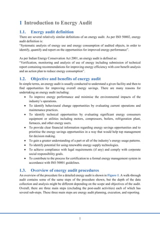
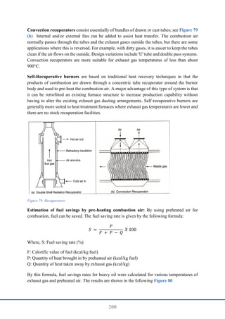
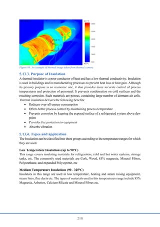
The document provides energy auditing and reporting guidelines developed for industries in Bhutan, aiming to improve energy efficiency by addressing consumption patterns and identifying energy conservation measures. It includes detailed procedures on various types of energy audits, data collection methods, and assessment techniques tailored for key equipment used in industries. The guidelines are intended to promote effective energy auditing practices, supported by practical templates and insights from extensive research and experience in energy audits.

1. 1
Energy Auditing and Reporting
Guidelines for Industries
Department of Renewable Energy,
Ministry of Economic Affairs,
Royal Government of Bhutan

2. i
Copyright
Copyright © The Department of Renewable Energy, Ministry of Economic Affairs, Royal
Government of Bhutan
This publication may be reproduced in whole or in part and in any form for educational or non-
profit purposes without special permission from the copyright holder, provided
acknowledgment of the source is made. Copyright holder would appreciate receiving a copy
of any publication that uses this publication as a source. No use of this publication may be
made for resale or for any other commercial purpose whatsoever without prior permission in
writing from the copyright holder.
Disclaimer
This report is intended solely for the purpose of drafting Energy Auditing and Reporting
Guidelines for Industries. Other parties should not rely upon the report or the accuracy or
completeness of any conclusions and should make their own inquiries and obtain independent
advice in relation to such matters.
All information provided by STENUM Asia in the report is done so in good faith and on an ‘as
is’ basis. The Department of Renewable Energy, Ministry of Economic Affairs, Royal
Government of Bhutan (DRE) and STENUM Asia makes no representation or warranty as to
the reliability, accuracy, or completeness of the information.
DRE or STENUM Asia and any related person accept no responsibility for any loss arising
from any action taken or not taken by anyone using this report.

3. ii
Acknowledgements
STENUM Asia is grateful to the Department of Renewable Energy (DRE), Ministry of
Economic Affairs, Royal Government of Bhutan who have contributed to the overall approach
and structure of these guidelines.
STENUM Asia would like to thank its local consortium partner – DESIGN Studio, Bhutan for
their support in this project. Their knowledge in the field of energy efficiency particularly for
the buildings sector in context of Bhutan was very useful in developing these guidelines.

4. iii
ནུས་ཤུགས་སླར་འབྱུང་ལས་ཁུངས། བསྟན་རྒྱས་ལྷན་ཁག།
དཔལ་ལྡན་འཔྲུག་གཞུང་། ཐིམ་ཕུག།
DEPARTMENT OF RENEWABLE ENERGY
MINISTRY OF ECONOMIC AFFAIRS
Royal Government of Bhutan
Thimphu : Bhutan
Foreword
The Department has conducted numerous studies to scrutinize the energy consumption pattern
of various energy intensive sectors in the Country. One such study was carried out in 2014
which revealed that the Buildings and the Industries are the major energy consuming sectors.
The Building sector alone consumed around 42 % of the total energy followed by Industries at
37 %1
The Department therefore sees potential for substantial energy savings through the
implementation of energy efficiency interventions in these sectors.
The major energy losses in the Bhutanese Industries occur due to the inefficient technologies
installed in the plant. Such inefficient technologies are known to be undermining the energy
efficiency of the equipment. Only a portion of the consumed energy produces a meaningful
output while rest is being wasted owing to its inefficiency. Thus, the energy consumption
pattern has to be evaluated to identify major causes of energy losses in the Industries.
Therefore, the Department deems it necessary and timely to develop the Energy Auditing and
Reporting Guideline for Industries to guide all the energy auditors and managers to conduct a
well-structured and effective energy audit.
The Department aspires that this guideline will promote the practice of energy auditing in
Bhutan and thus, contribute towards achieving optimum energy efficiency for the Industry
sector in the country.
Tashi Delek
Phuntsho Namgyal
Director
Department of Renewable Energy
Ministry of Economic Affairs
1
Energy Efficiency Roadmap 2019

5. iv
Executive Summary
These Energy Auditing and Reporting Guidelines for industries are designed to serve as a
practical guide for an energy professional to gain a strong background on energy auditing
through the detailed explanations on the components of an energy audit, the general methods
and procedures to be followed as well as the reporting practices of an effective energy audit.
A survey was conducted with several industries to determine their awareness level of energy
conservation practices. This survey along with detailed interactions with local experts from
industry and academia helped shape the structure of these guidelines. Chapter 2 of these
guidelines helps the reader select the type of energy audit most suitable for the industry, and to
prepare for the audit before commencing the audit.
These guidelines contain the information an energy auditor would need to assess and to identify
energy conservation measures for key energy consuming equipment commonly found at the
industries in Bhutan. For the benefit of the reader of these guidelines, this information is always
presented under six distinct sections for each of the equipment covered. The six sections are:
introduction to the equipment, data collection required for assessment of that equipment,
instruments required, performance terms and definitions, performance assessment techniques
and energy saving opportunities commonly associated with the specific equipment.
With this approach and the steps explained, an energy professional would be able to carry out
energy performance assessment of a wide variety of equipment and to identify energy
conservation measures best suited for the concerned industry.
The approach to conduct plant level energy use assessment is explained in Chapter 6, which is
followed by guidance on developing and use of benchmarks for energy efficiency in Chapter
7. The reader is explained various ways to carry out economic evaluation of identified energy
conservation measures in Chapter 8. These are particularly important for reporting to senior
management of industries. Chapters 9 and 10 guide the energy professional on optimum
reporting methods and on post audit evaluation and monitoring for effectiveness of the
implemented measures. In the concluding chapters of these guidelines, data collection
templates and energy saving calculation formulae and tips are provided to support the auditors.
The authors have practical experience of conducting over 700 energy audits in several countries
in South Asia. They have leveraged this experience and conducted detailed primary and
secondary research covering best energy management practices from seven countries, to
optimally balance theoretical background with practical inputs on how to carry out effective
energy audit at industries, especially for Bhutan.

6. v
Table of Contents
Copyright.............................................................................................. i
Disclaimer............................................................................................. i
Acknowledgements............................................................................. ii
Foreword ............................................................................................ iii
Executive Summary .......................................................................... iv
List of Figures .................................................................................. viii
List of Tables...................................................................................... xi
Acronyms.......................................................................................... xiii
1 Introduction to Energy Audit ....................................................1
1.1. Energy audit definition 1
1.2. Objective and benefits of energy audit 1
1.3. Overview of energy audit procedures 1
2 Types of Energy Audit and Approach......................................3
2.1. Walk-through energy audit 3
2.2. Targeted energy audit 5
2.3. Detailed energy audit 6
3 Preparation for Detailed Energy Audit ....................................7
3.1. Audit scope 7
3.2. Preliminary data collection 7
3.3. Audit plan 8
3.4. Introductory meeting 9
3.5. Initial walk-through visit 9
4 Conducting Detailed Energy Audit.........................................11
4.1. Process flow diagram 11
4.2. Comprehensive data collection 12
4.3. Energy bills analysis 13
4.4. Analysis of historical energy use and SEC 16

7. vi
4.5. Measurements, survey, and verification of measured data 19
5 Detailed Energy Performance Assessment.............................21
5.1. Electrical systems & Power Factor 21
5.2. Transformers 35
5.3. Motors and application of Variable Frequency Drive (VFD) 39
5.4. Air Compressors – energy performance assessment 58
5.5. Heating, ventilation, air conditioning & refrigeration systems 73
5.6. Fans and Blowers – energy performance assessment 96
5.7. Pumps – energy performance assessment 108
5.8. Cooling towers – energy performance assessment 122
5.9. Lighting system – energy performance assessment 134
5.10. Boilers – energy performance assessment 143
5.11. Furnaces & Ovens – energy performance assessment 167
5.12. Waste heat recovery 209
5.13. Insulation & refractories 217
5.14. Renewable energy systems 228
6 Analysis of Energy Use and Material Balance.....................239
6.1. Introduction 239
6.2. Purpose of energy and material balance 239
6.3. Component of energy and material balance 239
6.4. Basic principles of energy and material balance 240
6.5. Classification of process 241
6.6. Energy balance 246
7 Benchmarking .........................................................................249
7.1. Industrial benchmarking programs 249
7.2. Plant Energy Performance (PEP) 251
7.3. Production factor 251
8 Cost Benefit Analysis ..............................................................253
8.1. Payback period 253

8. vii
8.2. Return on Investment (ROI) 253
8.3. Net Present Value (NPV) 254
8.4. Internal Rate of Return (IRR) 256
8.5. Capital investment considerations 257
9 Detailed Energy Audit Reporting..........................................258
9.1. Typical contents of the report 258
10 Post Audit Activities................................................................266
10.1. Define technical Steps and targets 266
10.2. Determine roles and resources 266
11 Energy Audit Instruments .....................................................269
12 List of Simulation Software....................................................274
13 Annexures ................................................................................277
13.1. Compilation of audit checklist and energy savings tips 277
13.2. List of excel forms 281
13.3. Sample excel forms 282
14 References ................................................................................283

9. viii
List of Figures
Figure 1: Overview of detail energy audit procedure 2
Figure 2: An example of process flow chart 12
Figure 3: Historical electricity intensity patterns for a spinning mill 17
Figure 4: Historical fuel intensity pattern for a spinning mill 17
Figure 5: Visualisation of type of energy use in pie chart 17
Figure 6: An example of line graph depicting SEC over time 18
Figure 7: An example of line graph depicting SFC over time 18
Figure 8: An example of electricity consumption breakdown 19
Figure 9: Appropriate portable measuring instruments for various systems 20
Figure 10: Illustration of electricity transmission and distribution system 22
Figure 11: Hourly load curve 24
Figure 12: Reactive energy supplied and billed by the energy supplier or utility 25
Figure 13: Power triangle 26
Figure 14: Connection of capacitors at load level 27
Figure 15: No-load compensation for transformer 28
Figure 16: Power factor correction triangle 29
Figure 17: Different compensation modes for power factor improvement 32
Figure 18: Transformer losses as a percentage (%) of load (Source: UNEP) 37
Figure 19: Voltage unbalance (%) versus motor losses & motor heating (Source: BEE) 43
Figure 20: Effect of motor loading on efficiency & power factor (Source: BEE) 45
Figure 21: Effect of motor speed on power factor (Source: BEE) 45
Figure 22: Effect of motor loading on efficiency (Source: BEE) 46
Figure 23: Star connection 48
Figure 24: Delta connection 48
Figure 25: Method 1- Capacitor is connected directly to the motor 49
Figure 26: Method 2 - Capacitor is connected to the motor before starter 50
Figure 27: IE efficiency classes for 4 pole motors at 50 Hz (Source: ABB) 51
Figure 28: Component of VFD system 55
Figure 29: Example of an excellent variable speed drive candidate 57
Figure 30: Example of a poor variable speed drive candidate 57
Figure 31: Sankey diagram of compressed air losses 58
Figure 32: Types of compressors 59
Figure 33: Figure of elements of compressed air system 60
Figure 34: Heat Transfer Loops in refrigeration system 73
Figure 35: Psychrometric chart (Source: BEE) 75
Figure 36: Psychrometric chart depicting human comfort zone (Source: BEE) 76
Figure 37: Vapour compression refrigeration system 79
Figure 38: Benefit of automatic tube cleaning system (Source: Trane) 85
Figure 39: Effect of speed on power and air volume 89
Figure 40: Heat Pump working (Source: Aspiration energy) 92
Figure 41: Centrifugal fan (left) and axial fan (right) 97
Figure 42: Measurement by pitot tube 102

10. ix
Figure 43: Traverse on round and square duct areas 103
Figure 44: Pulley change 106
Figure 45: Centrifugal fan with induction motor 107
Figure 46: Plug fan with BLDC (single) 107
Figure 47: Plug fan with BLDC motors (combination) 107
Figure 48 System curve with high static head 108
Figure 49 System head with low static head 108
Figure 50: Head-Flow curve 109
Figure 51: Typical pump curve provided by manufacturer 109
Figure 52: Pump operating point 110
Figure 53: Before impeller trimming 116
Figure 54: After impeller trimming 116
Figure 55: Effect of speed change in a system with no static head 118
Figure 56: Effect of speed change in a system with high static head 119
Figure 57: Effect of VFD 120
Figure 58: Typical head-flow curve for pumps in parallel operation 121
Figure 59: Cooling tower with closed loop 122
Figure 60: Types of cooling tower (Source: BEE) 123
Figure 61: Range and Approach 125
Figure 62: Fire tube boiler 144
Figure 63: Water tube boiler (Source: BEE) 145
Figure 64: Packaged Boiler (Source: BEE) 146
Figure 65: Various heat losses in fuel fired Boiler 150
Figure 66: Blowdown heat recovery system 161
Figure 67: Different phases of induction furnace batch process (Source: SA) 169
Figure 68: Electric arc furnace - section and plan view (source: steeluniversity.org) 173
Figure 69: Material balance of EAF 175
Figure 70: Furnace losses 181
Figure 71: Furnace wall losses 182
Figure 72: Furnace opening losses 182
Figure 73: Air infiltration in furnace 183
Figure 74: Wrong Correct heat distribution in furnace 196
Figure 75: Correct heat distribution in furnace 196
Figure 76: Wrong alignment of burners 196
Figure 77: Correct alignment of burners 196
Figure 78: Effect of pressure on the location of zero level 198
Figure 79: Recuperators 200
Figure 80: Fuel savings rate by preheated air temperature (Source: BEE) 201
Figure 81: Fishbone diagram of fuel fired furnace 204
Figure 82: Typical industrial oven 205
Figure 83: Recuperator configuration 211
Figure 84: Metallic radiation recuperator 212
Figure 85: Tube type recuperator 213
Figure 86: Sketch of heat wheel 215

11. x
Figure 87: Economiser 216
Figure 88: An example of thermal image taken from thermal camera 218
Figure 89: Illustration of optimal insulation 220
Figure 90: Determination of economic thickness of insulation (Source: BEE) 221
Figure 91: High emissivity coatings of various insulating materials 227
Figure 92: Stand-alone PV system (Source: Apricus solar) 229
Figure 93: Direct Normal Irradiation map of Bhutan (Source: World bank group) 230
Figure 94: Global Horizontal Irradiation (Source: World bank group) 231
Figure 95: Effect of temperature change on power and voltage 235
Figure 96: Solar water heater 236
Figure 97: Energy and material balance representation 241
Figure 98: Classification of process 242
Figure 99: Conservation of energy 247
Figure 100: Efficiency and losses 247
Figure 101: Sankey diagram for Boiler fuel input to heat output 248

12. xi
List of Tables
Table 1: Energy savings recommendation table format for walk-through energy audit 5
Table 2: An example of data collection sheet for electricity bill 16
Table 3: Multipliers to determine capacitor kVAr requirements 30
Table 4: Effect of voltage unbalance on motor performance (source: BEE) 42
Table 5: Motor rating versus stray losses (adapted from IEEE) 47
Table 6: Equipment wise compressed air requirement 60
Table 7: Discharge of air (m3
/min) through Orifice 64
Table 8: Typical power savings through pressure reduction (Source: BEE) 65
Table 9: Effect of intake air temperature on power consumption (Source: BEE) 68
Table 10: Effect of pressure drop across air inlet filter on power consumption 69
Table 11: Moisture in ambient air at various humidity levels (Source: BEE) 69
Table 12: Typical pressure dew point and power consumption (Source: BEE) 70
Table 13: Effect of altitude on Volumetric Efficiency (Source: BEE) 71
Table 14: Typical power requirements for pneumatic and electrical Tools 71
Table 15: Effect of poor compressor maintenance in HVAC system 83
Table 16: Refrigerant phase-out dates 86
Table 17: Recommended air changes per hour 90
Table 18: Difference between Fan, Blowers and Compressor 96
Table 19: Fan efficiencies 96
Table 20: Types of fan, characteristics, and typical application 98
Table 21: Symptoms that indicate opportunity for energy saving 114
Table 22: Flow and approach for given tower 125
Table 23: Typical comparison between various fill media 128
Table 24: Determination of measurement points 135
Table 25: Target load efficacy (ILER) 136
Table 26: Indicators of performance 137
Table 27: Summary of lighting measurement 138
Table 28: Standard Lux level for plant (Source: IS 3646) 139
Table 29: Luminous performance characteristics of commonly used luminaries 141
Table 30: Typical instrument used for Boiler performance assessment 151
Table 31: Measured and collected parameter from a plant 156
Table 32: Recommended TDS levels for various industrial process Boilers 159
Table 33: Theoretical combustion data - common Boiler fuel (Source: BEE) 163
Table 34: Excess air levels for different fuels (Source: BEE) 163
Table 35: Coefficient based on the profile of furnace openings 193
Table 36: Specific heat of gases at constant pressure 193
Table 37: Air ratio for fuel fired furnaces 195
Table 38: Operating temperature of various furnaces 197
Table 39: Waste source and quality 210
Table 40: Thermal conductivities of typical hot insulation materials (Source: BEE) 219
Table 41: Fuel savings calculation 224
Table 42: Benchmarking parameters for various industries 250

13. xii
Table 43: Summary of energy savings recommendation format 260
Table 44: Types and priority for energy savings measure format 261
Table 45: Energy savings recommendation format 263

14. xiii
Acronyms
AC Alternating Current
BEE Bureau of Energy Efficiency
COP Coefficient of Performance
DC Direct Current
DRE Department of Renewable Energy
EAF Electric Arc Furnace
EER Energy Efficiency Ratio
FAD Free Air Delivery
HVAC Heating, Ventilation, Air Conditioning
IE International Efficiency
IEC International Electrotechnical Commission
IEEE Institute of Electrical and Electronics Engineers
IR Infra-Red
IRR Internal Rate of Return
ISO International Organisation for Standardisation
MD Maximum Demand
PF Power Factor
ROI Return on Investment
SA STENUM Asia Sustainable Development Society
SEC Specific Energy Consumption
Solar PV Solar Photo Voltaic
UNEP United Nations Environment Programme
VFD Variable Frequency Drive
VSD Variable Speed Drive
Units
°C Degree Celsius
A Ampere
hr hours
kcal kilo calorie
kg kilogram
kJ kilo Joules
kl kilo litre
kVA kilo Volt Ampere
kVAr kilo Volt Ampere reactive
kWh kilo Watt hour
l litre
m meter
t ton
toe tonne of oil equivalent
TR Tonne of Refrigeration
V Volt

15. 1
1 Introduction to Energy Audit
1.1. Energy audit definition
There are several relatively similar definitions of an energy audit. As per ISO 50002, energy
audit definition is:
“Systematic analysis of energy use and energy consumption of audited objects, in order to
identify, quantify and report on the opportunities for improved energy performance”.
As per Indian Energy Conservation Act 2001, an energy audit is defined as:
“Verification, monitoring and analysis of use of energy including submission of technical
report containing recommendations for improving energy efficiency with cost benefit analysis
and an action plan to reduce energy consumption”.
1.2. Objective and benefits of energy audit
In simple terms, an energy audit is usually conducted to understand a given facility and then to
find opportunities for improving overall energy savings. There are many reasons for
undertaking an energy audit including:
 To improve energy performance and minimise the environmental impacts of the
industry’s operations.
 To identify behavioural change opportunities by evaluating current operations and
maintenance practices.
 To identify technical opportunities by evaluating significant energy consumers
equipment or utilities including motors, compressors, boilers, refrigeration plant,
furnaces, and other energy users.
 To provide clear financial information regarding energy savings opportunities and to
prioritise the energy savings opportunities in a way that would help top management
for decision making.
 To gain a greater understanding of a part or all of the industry’s energy usage patterns.
 To identify potential for using renewable energy supply technologies.
 To achieve compliance with legal requirements (if any) and comply with corporate
social responsibility goals.
 To contribute to the process for certification to a formal energy management system in
accordance with ISO 50001 guidelines.
1.3. Overview of energy audit procedures
An overview of the procedure for a detailed energy audit is shown in Figure 1. A walk-through
audit contains some of the same steps of the procedure shown, but the depth of the data
collection and analysis might be different depending on the scope and objectives of the audit.
Overall, there are three main steps (excluding the post-audit activities) each of which has
several sub-steps. These three main steps are energy audit planning, execution, and reporting.

16. 2
Plan and organise
Introductory meeting
Data collection & understanding process
flow
Measurements and survey
Detail performance assessments of
equipment & Utilities
Analysis of energy use and material
balance
Identification & development of energy
savings opportunities
Cost benefit analysis
Post audit action plan and implementation
monitoring
Reporting and presentation to the top
management
Plan
Execute
Report
Post audit
activities
Figure 1: Overview of detail energy audit procedure

17. 3
2 Types of Energy Audit and Approach
The type of energy audit to be performed depends on the type of industry, the depth to which
final audit is needed, and the potential and magnitude of cost reduction desired. Thus, an energy
audit can be classified into the following types: walk-through energy audit, targeted energy
audit and detailed energy audit.
2.1. Walk-through energy audit
In a walk-through energy audit, readily available data are mostly used for a simple analysis of
energy use and performance of the plant. This type of audit does not require a lot of
measurement and data collection. These audits take a relatively short time and the results are
more general, providing common opportunities for energy efficiency. The economic analysis
is typically limited to calculation of the simple payback period.
Objectives of walk-through energy audit
 Identification and basic evaluation of low-cost opportunities that can be easily
implemented.
 Understanding of energy consumption at an industry or equipment/utility level
 Improved awareness of energy costs and the potential benefits of managing energy
 Understanding of the extent of more capital-intensive opportunities.
 Indications of potential savings and benefits from undertaking more detailed investigations
such as targeted or detailed energy audit.
The savings potential identified from conducting a walk-through audit can help the clients to
determine whether they should proceed to undertake targeted audit or a detailed audit.
Simultaneously, a walk-through audit helps the audit team to prepare a more effective audit
plan (which includes composition of audit team and allocation of time or certain section of
client facility, selection of instruments to carry) when proceeding with targeted or detailed
audit.
Preparations for walk-through energy audit and resources required
Walk-through audit by itself can give significant benefits, provided it is carried out by an
experienced energy audit team as limited time and resources are available and detailed
measurements are not feasible.
Resources required
1. Team: 1 to 2 members
2. Basic instruments for quick assessments (if available) such as:
 Non-contact type Infra-red thermometer,
 Hand-held clamp meter
 Pen-type thermometer
 Sling Psychrometer
 Anemometer
 Measuring tape
 Electric tester, etc.

18. 4
Refer Chapter 11 for list of instruments and their usage.
3. Others
 Data collection format
 Audit checklist,
 Log sheet
 Diary/notebook
Process of carrying out walk-through energy audit
1. Introductory meeting
The walk-through audit generally begins with an introductory meeting with industry
management personnel. The purpose of the preparatory meeting is to understand the industry
and major processes before actual visit to the shop floor or plant so that the audit goals reflect
the operations of the industry. The energy auditor shall start the meeting with a short
presentation apprising the management about the audit goals and possible benefits to the
industry. The energy auditor shall take the management views on which aspects of operation
should be the focussed area during the audit and shall identify the key issues of the clients. The
energy auditor shall collect energy consumption (electricity and fuel bills for 12 months) and
corresponding production data (for same 12 months). The energy auditor shall try to get a
detailed description of industry process, significant energy consumers, type of products and
other general information.
2. Walk-through
The next step is to walk-through the industry with appropriate plant personnel who is familiar
with all the installed equipment and utilities related operation. During walk-through, the energy
auditor then identifies key issues of the client and gather inputs on the areas of concern, record
observations, note the nameplate and meter readings, identify low cost and easily
implementable energy savings measures. The energy auditor shall ensure covering all
functional areas while conducting a walk-through.
The reader may refer audit checklist given in Annexure-13.1 to select appropriate and relevant
energy savings opportunities that may be applicable.
3. Closing meeting
The energy auditor shall hold a short wrap-up meeting to review main points observed during
the walk-through, highlight any observation or finding which needs immediate attention by
industry management. Fix the date for walk-through audit report presentation and submission
with industry management.
4. Analysis & report preparation
Start analysing the collected data, reviewing the notes taken during the walk-through, and start
preparing the energy savings recommendations. Recommendations to industry should be
specific and supported by data to the extent possible and presented in order of monetary savings
(highest savings on top or shortest return on investment on top). These should contain estimated

19. 5
costs (checked from local market), estimated savings and simple payback calculations.
Consider the priority set by industry while preparing the walk-through audit report.
5. Report presentation and action plan
The energy auditor shall personally hand over the walk-through audit report to the industry on
the agreed date, explaining the recommendations made to the top management. The energy
auditor shall help the industry management to prepare an action plan with selection of
recommendations along with timeline for implementation.
Typical content of Walk-through energy audit report
1. Executive Summary
 Summary of energy savings potential
 Recommendations breakup in payback and savings categories
2. Current Industry Situation
 Industry processes
 General information on energy consumption
 Energy and production data analysis
3. Energy Savings recommendations in format as shown in Table 1
4. Annexure
Table 1: Energy savings recommendation table format for walk-through energy audit
Sl.
No.
Description
of the
present
situation
and the
problem
observed
Description of
recommended
actions
Amount of the annual
savings
Estimated
Investment
Costs (Nu.)
Simple
payback
period
(months)
Energy
savings
(kWh/year or
kl/year) (as
appropriate)
Amount
(Nu.
/year)
2.2. Targeted energy audit
The need for targeted energy audits often identified pursuant to a detailed analysis of the results
of a walk-through audit with client / management. The targeted audits provide data and detailed
analysis on specified target projects. For example, an organization may target its lighting
system or boiler system or steam system or compressed air system with a view of effecting
energy savings.
Targeted audits therefore involve detailed surveys of the target subjects and analysis of the
energy flows and cost associated with the targets. Final outcome is the recommendations
regarding actions to be taken for energy conservation. Detail on how to carry out targeted audit
on certain utilities or equipment are provided in respective sections under Chapter 5

20. 6
2.3. Detailed energy audit
Detailed energy audit is a comprehensive audit and results in a detailed energy project
implementation plan for a facility since it accounts for the energy use of all major equipment.
It considers the interactive effects of various projects and offers the most accurate estimate of
energy savings and cost. It includes detailed energy cost saving calculations and project
implementation costs. One of the key elements in a detailed energy audit is the energy balance.
This is based on an inventory of energy-using systems, assumptions of current operating
conditions, measurements, and calculations of energy use. Detailed energy auditing is carried
out in three phases as shown in Figure 1.

21. 7
3 Preparation for Detailed Energy Audit
3.1. Audit scope
As per ISO 50002, definition of scope is “activities the energy auditor and the organisation
agree are necessary for the energy audit”.
The audit scope needs to consider the available resources such as staff, time, audit boundaries,
level of analysis, expected results, the degree of detailing, and the budget for conducting the
energy audit. The audit scope will depend on the purpose of the specific audit and may be
defined by an overall government or company audit program. It should also define the share of
processes included in the audit of the industry’s total energy use as well as comprehensiveness
and the level of detail for the final recommendations. Therefore, the scope of the audit may be
defined in terms of the processes to be covered or the areas or sections of the industry that need
to be covered, from within the entire industry. In many cases the entire industry would be the
scope of the audit.
It is responsibility of the energy auditor to clarify and define the scope of the energy audit
before starting the audit, by considering all the points mentioned in previous paragraph.
3.2. Preliminary data collection
Energy bills along with other current and historical energy and production related data and
information should be collected at the beginning of the audit process to analyse power
consumption pattern and anomalies therein. The more historical data available, the better the
auditor can understand the performance of the plant at differing times of day, in various
seasons, and under diverse production conditions. The suitable time to conduct energy audit in
an industry is over the period when the industry is running at its highest production output or
close to highest production capacity. The collected preliminary data will give some indication
of appropriate time duration for completing an effective energy audit.
The data that can be collected at the beginning of an energy audit may include the following:
 Month wise electricity bills and fuel bills for the last 1 to 2 years
 Monthly production data for the same period
 List of major energy consuming equipment with their nameplate ratings.
 Status of energy management and any energy-saving measures implemented in the
recent past (by the industry on their own or as part of external consultancy or agency
driven improvement programme).
 General information about the plant (year of construction, ownership status,
renovations, types of products, operation schedule particularly for certain equipment
that does not operate throughout the operating shifts, operating hours, scheduled
shutdowns, etc.)
The energy auditor shall study and analyse the collected preliminary data from audit planning
point of view.

22. 8
3.3. Audit plan
An audit plan outlines the audit strategy and procedure. The plan helps the auditors to check
the consistency and completeness of the audit process and ensure that nothing important is
neglected or overlooked. The audit plan, after taking into consideration the preliminary data
collected, should provide the following
 Scope of the audit
 Time of the audit and its duration as well as the timeline for each step of the audit
process
 Elements of the audit that have a high priority
 Responsibilities and tasks of each audit team member
 Format of the audit report and its outline
Selection of energy audit team
Upon reviewing the collected preliminary data and defining the audit scope, a competent team
for energy audit shall be constituted. The team competence can be shown by:
 Appropriate education and/or training for energy audit
 Relevant technical, managerial, and professional experiences and skills
 Familiarity with appropriate local regulations, and energy auditing & reporting
guidelines
 Familiarity with the energy equipment, utilities and process being audited
 Familiarity with energy audit instruments and competent enough to operate and handle
the energy audit instruments safely.
In case, any of above-mentioned criteria are not met within the available team, an external
professional may be hired/consulted to be part of the audit team.
It is a good practice to prepare a documented audit plan and to share it with the industry client
upfront. To the extent possible the audit team should follow the audit plan, however, in view
of new observations / issues notice or ground situation changes, the audit plan may be modified
during the audit. In such cases, the updated audit plan may be shared with the client
subsequently.
Safety considerations
Ensure that relevant personal protective equipment (PPE) is available to all team members.
Commonly relevant PPEs are: Electrical safety gloves, industrial safety boots, heat resistant
furnace gloves, face masks, protective eyewear, safety helmet (hard hat). Loose clothing (such
a necktie or shawl) is to be strictly avoided to safely operate plant(s) and machineries to prevent
accidents at site.
It is strongly recommended to comply with the health and safety guideline and procedures as
defined by the relevant local authorities.
Energy auditors must ensure their own safety by following safe practices while carrying out
energy audits. Following safe pathways, not touching objects that may be hot, keep safely away

23. 9
from any live wires, cables and other conductive surfaces are a few basic safety considerations
that must be followed at all times by the auditors. Moreover, the auditors need to study and put
into practice all the relevant safety considerations on their own at each site and in each audit
depending upon the nature of activities undertaken by the clients.
3.4. Introductory meeting
The purpose of the introductory meeting is to set the context for the energy audit, confirm its
scope, engage all relevant industry personnel in the audit process and request specific
additional energy information from the industry. This information should enable appraisal of
the client organisation’s current energy use and energy management system.
In the introductory meeting, the energy auditor shall request the industry to:
 Identify a person to liaise with the energy auditor, where necessary supported by other
appropriate individuals constituted as a team for the purpose.
 Inform all the divisional engineering heads and other interested parties about the energy
audit and any requirements placed on them in connection with it.
 Disclose any unusual conditions, maintenance work or other activities that will occur
during the energy audit.
 Ensure cooperation of the engineering team and other interested parties.
 Nominate a management representative to take responsibility for evaluation and
implementation of energy performance improvement measures identified during the
audit.
The energy auditor shall agree with the organization on:
 Arrangements for access to the audited objects for the energy auditor.
 Health, safety, security and emergency rules and procedures.
 Resources and data to be provided
 Proposed visit and other schedules
 Requirements for special measurements, if needed
 Procedures to be followed for installation of measuring equipment, if needed
 Aspects of data confidentiality (pertaining to the data already provided or yet to be
collected), if required.
The energy auditor shall share the audit plan, describe the processes, means and schedule of
the energy audit and the possible need for additional metering equipment.
3.5. Initial walk-through visit
The purpose of the initial walk-through visit is for the energy audit team to become familiar
with the industry to be audited. The auditors shall go through the processes and utilities that
they will audit in detail later.
The audit team shall also meet with the managers of the areas to be audited to provide an
introduction and establish a common understanding of the audit process. The auditors can

24. 10
solicit comments from the facility staff and can collect readily available data during the walk-
through visit. The outcome of this visit should be:
1. To finalise the energy audit team
2. To identify the main energy consuming areas/plant items to be surveyed in detail during
the audit.
3. To identify and prepare list of specific instruments required for energy audit
4. To collect macro data on plant energy resources, major energy consuming equipment.
5. To build up awareness and support for detailed energy audit.
6. To update the audit plan, if necessary.

25. 11
4 Conducting Detailed Energy Audit
4.1. Process flow diagram
An overview of unit operations, important process steps, material and energy use and waste
generation should be assembled in the form of process flow diagram. This visualisation of the
process flow, along with identification of energy input and output flows, helps the energy
auditor to identify energy saving potential to focus on during the detailed audit. Information
from existing drawings, records and shop floor surveys will help in preparing the flow chart.
Simultaneously the team should identify the various inputs and outputs streams at each process
step. An example of process flow chart of re-rolling mill (highlighting input resources and
outputs) is shown below:
Resources Process Wastes & Hazards
Prime Billet Receiving and Storing Rust Iron, Iron Scales
Electricity Billet Shearing Iron Scale
Rejected billets
Electricity Feeding to the furnace Iron Scale
Electricity
Furnace Oil
Heating
(In the furnace)
Heat
Electricity Automatic Rolling
Iron dust, Heat, Fumes
Rejected pieces
Electricity End Cutting
Process Waste
Heat
Compressed air
Water
Electricity
Quenching Heat
Waste, water

26. 12
Electricity
Quality Inspection
(Hardness test, tensile test)
Rejected products
Electricity
Steel wire for
bundling
Bundling and Weighing
Cut pieces
TMT BAR
Figure 2: An example of process flow chart
It may be noted that waste heat and rejection (rejection is not directly related to energy
consumption, but it is leading to rework and increased energy consumption of mill) has been
identified at various stages in this flow chart. The audit focus will depend upon consumption
of input resources, energy efficiency potential, impact of process step on entire process or
intensity of waste generation/energy consumption.
4.2. Comprehensive data collection
Based on the preliminary data collection, the energy auditor shall prepare a customised data
collection spread sheet to suit the industry type. The data collection spread sheet shall have
clear and descriptive headings with appropriate rows and columns for different energy
consumers. A general data collection sheet shall be avoided as it will not serve meaningful
purpose.
In addition to data collected at preliminary data collection stage, the energy auditor shall also
collate the following information during energy audit:
 List of energy consuming systems, processes, and equipment
 Detailed characteristics of the audited object(s) including known relevant variables and
how the organization believes they influence energy consumption
 Current and historical data of:
o energy consumption
o relevant variables
o relevant related measurements
 Monitoring equipment configuration, and analysis information such as local gauges,
distributed control systems, instrumentation types.
 Future plans that affect energy use such as planned expansions, contractions or changes
in production volume or planned changes in replacement of equipment or systems that
have significant energy implications.
 Design, operation and maintenance documents
 Energy audits or previous studies related to energy and energy performance
 Current or a reference tariff of electricity and fuel to be used for financial analysis and
other relevant economic data

27. 13
 Knowledge on how the organization manages its energy and relative configuration of
the energy distribution system and the management structure
The data collected should be comprehensive enough to determine the energy baseline period.
Energy baseline period is a suitable period in which the organisation account for operating
cycles, regulatory requirements or variables that affect the energy consumption and energy
efficiency, so that the data period adequately demonstrates a full range of performance. Data
that the industry has, can be data what it has internally generated (e.g. through measurements,
log sheets) or data which it has access to electricity bills, fuel bill and annual reports).
Energy reduction target year: The industry management may have established quantifiable
objectives of energy performance improvement. If so, there would be some data analysis done
by the industry to develop, track the energy reduction over a period. Review of this data would
help the energy auditor determine further opportunities for energy saving as well as to obtain
insights into the industry’s focus and approach to energy conservation.
Difference between sales figures and production figures
While analysing the energy consumption of an industry over a period of time, it is important
to relate energy consumption to production output. It is understandable that in period of high
production output, higher energy consumption may be needed. However, it is the energy
auditor’s task to analyse the relationship between production figures and energy consumption.
Sometimes the industry may provide their monthly sales or despatch figures rather than the
actual month by month production figures, since the latter are not maintained well.
Sales figures may be significantly different from production figures due to storage or carrying
inventories. Hence energy audits prefer to use actual production figures to compare energy
consumption. In case the inventory levels are small or are nearly constant over the months
under study, sales figures may be treated as a proxy for production figures.
4.3. Energy bills analysis
Understanding energy costs
Contrary to common belief, energy costs are not a fixed overhead, there is often a huge
potential for cost savings, understanding energy cost is a vital factor for awareness creation
and savings calculation. In some industries, sufficient meters may not be available to measure
all the energy used. In such cases, bills for fuels and electricity will be useful. The annual
company balance sheet is the other sources where fuel cost and power are given with
production related information.
Energy bills shall be analysed by auditor since they:
● Provide a record of energy purchased in a given year which gives a baseline for future
reference
● Indicate the potential for savings when related to production requirements.
● Provide the basis of maximum demand tariff.
● Allow comparison of energy cost (and changes in energy consumption) over time.

28. 14
Fuel costs
Following are the most common types of fuels used in Bhutan for thermal energy supply are
● Diesel
● Coal
● Furnace oil
Understanding fuel cost is simple and it is purchased in tons (t) or kilolitres (kl) and generally
defined in Tonnes of Oil Equivalent (TOE). The three main factors that affect the fuel costs
are:
● Price at source, transport charge, type of transport
● Quality of fuel (contaminations, moisture, etc.)
● Energy content of fuel (calorific value)
The main components of fuel bills are:
1. Quantity (kl or kg)
2. Price (Nu.) including transportation cost
3. Calorific value of fuel
The calorific value of the fuel is the key parameters while analysing actual energy consumption,
rather than simply considering the procurement quantity (e.g. 1 t of low calorific value coal
may have less embodied energy than 0.8 t of high calorific value coal).
Electricity bill analysis
The electricity billing by utilities for medium and large industries is often done on two-part
tariff structure, i.e. one part for capacity (power or demand) drawn and the second part for
actual energy drawn during the billing cycle. Capacity or demand is in kVA (apparent power)
or kW terms. The reactive energy, i.e. kVAr drawn by the service is also recorded and billed
for in some utilities, because this would affect the load on the utility. Accordingly, utility
charges for maximum demand, active energy, and reactive power drawn (as reflected by the
power factor) in its billing structure. In addition, other fixed and variable expenses are also
levied.
The tariff structure generally includes the following components:
 Maximum demand Charges also called as normative availability of a power plant,
relates to the maximum demand registered during month/billing period and
corresponding rate of utility.
 Energy Charges relate to energy (kilowatt hours) consumed during month or billing
period and corresponding rates, often levied in slabs of use rates.
● Power factor penalty or bonus rates, as levied by most utilities, and includes cost of
reactive power drawn from the grid.
 Time of day (TOD) rates like peak and non-peak hours are also prevalent in tariff
structure provisions of some utilities.

29. 15
 Penalty for exceeding contract demand. Contract demand means the maximum
amount of apparent power (kVA) demand that the customer expects to use and for
which the customer has contracted the utility.
 Any other charges, taxes, or subsidy as applicable.
Analysis of utility bill data and monitoring its trends helps energy auditors to identify ways for
electricity bill reduction through available provisions in the tariff framework.
The utility employs an electromagnetic or electronic tri-vector meter, for billing purposes. The
minimum outputs from the meters are:
 Maximum demand registered during the month, which is measured in pre-set time
intervals (15- or 30-minute duration) and this is reset at the end of every billing cycle.
 Active energy in kWh during billing cycle
 Reactive energy in kVArh during billing cycle
 Apparent energy in kVAh during billing cycle
It is important to note that while maximum demand is recorded, it is not the instantaneous
demand drawn, as is often misunderstood but the time integrated demand exceeding the
predefined cycle, that in fact gets recorded.
As an example, in an industry if the drawl over a recording cycle of 30 minutes is:
1. 2500 kVA for 4 minutes
2. 3600 kVA for 12 minutes
3. 4100 kVA for 6 minutes
4. 3800 kVA for 8 minutes
The energy meter will be computing maximum demand as:
(2500 𝑋 4) + (3600 𝑋 12) + (4100 𝑋 6) + (3800𝑋 8)
30
= 3603.7 𝑘𝑉𝐴
The month’s maximum demand will be the highest among such demand values recorded over
the month. The energy meter registers only if the value exceeds the previous maximum demand
value and thus, even if, average maximum demand is low, the industry has to pay for the
maximum demand charges for the highest value registered during the month, even if it occurs
for just one recording cycle duration i.e. 30 minutes during whole of the month.
Electricity Bill data collection: An energy auditor shall try to collect electricity bill data in a
prescribed spread sheet format for analysis as shown in below example Table 2

30. 16
Table 2: An example of data collection sheet for electricity bill
Month
& Year
Maximum
Demand
(kVA)
Energy
consumption
(kWh)
Power
Factor
(PF)
Maximum
Demand
charges
(Nu.)
Energy
charges
(Nu.)
Total
bill
(Nu.)
Effective
rate2 (Nu.
per kWh)
Jan-XX
Feb-XX
……
……
Dec-XX
Based on the components in electricity bill for the industry being audited, more columns can
be added or removed from the above table.
4.4. Analysis of historical energy use and SEC
Graphical analysis of historical energy use in a plant can help to better understand the energy
use pattern in the plant. Sometimes the patterns are unexpected and can lead to opportunities
to modify the way energy is used and thereby save energy. For example, one might not
normally expect a heavy process industry like cement industry to exhibit a seasonal variation
in energy use because of weather changes. Despite this, if a seasonal pattern shows up in the
graphical analysis, this may suggest the need to investigate for the possible sources of energy
losses. It is common for a plant’s operating conditions or capacities to vary over the year.
Therefore, the variation of energy use alone may not truly reflect the condition of energy
efficiency in a plant. Thus, it is much better and more accurate to conduct this type of graphical
analysis of a plant’s specific energy consumption (SEC), which is the energy use per unit of
output or production. SEC can be calculated by using monthly energy consumption data
obtained from energy bills and the monthly production data (using the appropriate unit of
production measurement). For example:
SEC = Energy consumption (kWh) / Production (t)
2
Total electricity bill amount for the month divided by total energy consumed in the month (Nu./kWh)

31. 17
A hypothetical example of specific electrical consumption for electricity and specific fuel
consumption in a textile spinning plant in a four-season country is provided in Figure 3 As can
be seen, the electricity intensity pattern over one year does not vary much, whereas the fuel
intensity pattern Figure 4 varies by the change in seasons. The reason is that in a spinning
plant, fuel is used just for heating during the cold months, as the temperature and moisture of
the ambient air of spinning plants needs to be kept constant all over the year.
A pie chart is another type of chart that can be used for graphical analysis of historical energy
use and cost data. A pie chart can be used to show the share of various types of energy use and
their costs graphically. Both monthly and annual data can be used for plotting such graph.
Figure 5 shows a hypothetical example of the share of each type of final energy use of one
year
Figure 5: Visualisation of type of energy use in pie chart
Line graphs can be used to depict tends over time. A useful line graph can be one depicting
SEC over period of time. Using a two-axis line graph is a good way to compare two parameters
over same time period. As the example in Figure 6 shows, the left side y-axis (green line)
depicts SEC while the right-side y-axis (blue line) depict total production over the Jan to Dec
time period. Here one can see that in months with high production, the SEC is low, and that
SEC varies in range of ~20 kWh/t over the period. Indicating that perhaps the industry is not
Electricity
61%
Diesel 28%
Coal 11%
Energy use breakdown
Electricity Diesel Coal
0.0
5.0
10.0
15.0
20.0
25.0
30.0
Jan Feb Mar Apr May Jun Jul Aug Sep Oct Nov Dec
Specific
fuel
consumption
(kl/t)
Month
0.0
2.0
4.0
6.0
8.0
10.0
Specific
electricity
consumptoin
(kWh/t)
Month
Figure 3: Historical electricity intensity patterns for a
spinning mill
Figure 4: Historical fuel intensity pattern for a spinning
mill

32. 18
normally running at optimum production levels. By observing the trend line of the SEC, one
notices that SEC has a rising trend even when production shows an increasing trend, which is
not desirable.
Figure 6: An example of line graph depicting specific electricity consumption (SEC) over time and increasing
trend of SEC
Figure 7: An example of line graph depicting specific fuel consumption (SFC) over time and decreasing trend of
SFC
In another similar example of a two-axis line graph shown in Figure 7, the SEC trend line
shows a small positive (lower SEC) trend, even with stable production over the period. This
may indicate some small improvement measures or good practices being implemented by the
industry over the period.
0
1,000
2,000
3,000
4,000
5,000
6,000
7,000
105
110
115
120
125
130
135
140
145
Jan Feb Mar Apr May Jun Jul Aug Sep Oct Nov Dec
Total
Production
(t)
Specific
electricity
consumption
(kWh/t)
Specific electricity consumption Total Production Linear (Specific electricity consumption)
0
1,000
2,000
3,000
4,000
5,000
6,000
7,000
40
41
42
43
44
45
46
47
48
49
Jan Feb Mar Apr May Jun Jul Aug Sep Oct Nov Dec
Total
Production
(t)
Specific
electricity
consumption
(kWh/t)
Specific fuel consumption Total Production Linear (Specific fuel consumption)

33. 19
4.5. Measurements, survey, and verification of measured data
Gathering data through measurement and survey is one of the main activities of energy
auditing. Without adequate and accurate data, an energy audit cannot be successfully
accomplished. Some data are readily available and can be collected from different divisions of
the plant being audited. Some other data can be collected through measurement and recording.
Electrical load inventory
Making an inventory of all electrical loads in a plant aims to answer two important questions:
 where the electricity is used?
 How much and how fast is electricity used in each category of load?
One way to prioritize the search for electricity-saving opportunities is by the magnitude of the
loads (kW). Therefore, identifying and categorizing different loads in a plant can be useful.
Often, the process of identifying categories of use allows energy waste to be easily identified,
and this frequently leads to low-cost savings opportunities. Identifying high-consumption loads
lets the auditor consider the best savings opportunities first. Because the inventory also
quantifies the demand (i.e. how fast electricity is used) associated with each load or group of
loads, it is invaluable for further interpretation of the demand profile. An example of electricity
consumption breakdown is shown in Figure 8
Verification of the measured data
Verify the measured values of the equipment and utilities with rated parameters of the
respective equipment and utilities and if a very wide variation observed between measured
values and rated parameters, this is an indication of following:
 The equipment or utility under observation is faulty and immediate attention is needed
by the facility engineering team.
 The equipment or utility under observation is partially loaded or not fully utilised, the
energy auditor shall investigate further to find energy saving opportunities.
70%
15%
8%
5% 2%
Electricity consumption breakdown
Induction furnace
Compressor
Water pumping
Cooling towers
Lighting
Figure 8: An example of electricity consumption breakdown

34. 20
 The method of measurement used by energy auditor may be wrong. Energy auditor
shall check whether their instruments are functioning well and shall take the
measurements again to verify.
Portable measuring instruments for energy audit
The energy audit team should be well-equipped with all the necessary measurement
instruments. The instruments used for measurements shall be well calibrated with valid
calibration certificate and functioning properly. Modern portable meters can store data
collected for a longer duration (24 hours or more) and can then be uploaded either directly or
remotely for analyses off site.
The energy auditor shall ensure:
 The instruments are well calibrated, and their calibration certificates are valid.
 The instruments calibration certificates are attached/pasted on the instruments
 The instruments are functioning well and safe to operate.
Refer Chapter-11 for detailed list of instruments required for energy audit.
Figure 9: Appropriate portable measuring instruments for various systems

35. 21
5 Detailed Energy Performance Assessment
5.1. Electrical systems & Power Factor
Introduction
The network through which the consumers get electricity from the source is called electrical
supply system. An electrical supply system consists of generating units that produce electricity,
high voltage transmission lines that transport electricity over long distances, and distribution
lines that deliver electricity to consumer.
Figure 10 is an illustration of electricity transmission and distribution system, and linkages
from electricity sources to end user.
The power generation units typically produce 50 Hertz alternating current (AC) electricity with
voltages between 11 kV and 33 kV. At the power generation units, the three-phase voltage is
stepped up to a higher voltage for transmission on cables strung on cross country towers. Extra
high voltages (EHV) like 265 kV to 275 kV and high voltages (HV) like 110 kV, and above
transmission is the next stage from power generation units to transport A.C. power over long
distances. Sub-transmission network at 132 kV, 110 kV, 66 kV or 33 kV constitutes the next
link towards the end user. Distribution at 11 kV/6.6kV/3.3 kV constitute the last link to the
consumer, who is connected directly or through transformers depending upon the drawn level
of service.
The transmission and distribution network include sub-stations, lines and distribution
transformers. High voltage transmission is used so that smaller, more economical wire sizes
can be employed to carry the lower current and to reduce losses. Sub-stations, containing step-
down transformers, reduce the voltage for distribution to industrial users.
There is no difference between a transmission line and a distribution line except for the voltage
level and power handling capability. Transmission lines are usually capable of transmitting
large quantities of electric energy over great distances. They operate at high voltages.
Distribution lines carry limited quantities of power over shorter distances.
Voltage drops in line are in relation to the resistance and reactance of line, length and the
current drawn. For the same quantity of power handled, lower the voltage, higher the current
drawn and higher the voltage drop. The current drawn is inversely proportional to the voltage
level for the same quantity of power handled.
The power loss in line is proportional to resistance and square of current. (i.e. P = I2
R). Higher
voltage transmission and distribution thus would help to minimize line voltage drop in the ratio
of voltages, and the line power loss in the ratio of square of voltages. For instance, if
distribution of power is raised from 11 kV to 33 kV, the voltage drop would be lower by a
factor 1/3 and the line loss would be lower by a factor (1/3)2
i.e., (1/9). Lower voltage
transmission and distribution also calls for bigger size conductor on account of current handling
capacity needed.

36. 22
Figure 10: Illustration of electricity transmission and distribution system (Source: UNEP)
Data collection
Following data shall be collected during audit with support from plant supervisor:
 Electricity Bill for preceding 12 months (minimum)
 Log sheet related to electrical fault caused by overheating or overvoltage
 Any recurring electrical faults recorded by plant supervisor
In addition to above, the following data shall be collected through measurements
 Power logging at mains panel up to 24 hours (duration of logging should be decided
mutually with plant supervisor)
 Power measurements at sub-panels
 Thermal images of inside electrical panels (to check overheating)

37. 23
Instruments required
 Three-phase power analyser
 Hand-held clamp meter
 Thermal imaging camera (to check overheating inside electrical panels)
Observation parameters
 Maximum demand or Peak demand
 Power factor
Measurements
The following electrical parameters can be measured using hand-held clamp meter or three-
phase power analyser.
 Voltage (V)
 Current (A)
 Power (kW)
 Power factor (PF)
 Apparent power (kVA)
 Reactive power (kVAr)
 Harmonics
 All other electrical parameters
Electrical load management and maximum demand control
Need for Electrical Load Management: In a macro perspective, the growth in the electricity
use and diversity of end use segments in time of use has led to shortfalls in capacity to meet
demand. As capacity addition is costly and only a long-time prospect, better load management
at user end helps to minimize peak demands on the utility infrastructure as well as better
utilization of power plant capacities. The utilities (Distribution companies) use power tariff
structure to influence end user in better load management through measures like time of use
tariffs, penalties on exceeding allowed maximum demand, night tariff concessions etc. Load
management is a powerful means of efficiency improvement both for end user as well as utility.
As the demand charges constitute a considerable portion of the electricity bill, from user angle
too there is a need for integrated load management to effectively control the maximum demand.
Step by Step Approach for Maximum Demand Control
1. Load Curve Generation
Presenting the load demand of a consumer against time of the day is known as a 'load curve'.
If it is plotted for the 24 hours of a single day with the help of a three-phase power analyser,
it is known as 'hourly load curve’ and if daily demands plotted over a month, it is called ‘daily
load curve’. A typical hourly load curve for an engineering industry is shown Figure 11.

38. 24
Figure 11: Hourly load curve
These types of curves are useful in predicting patterns of drawl, peaks and valleys and energy
use trend in a section or in an industry or in a distribution network as the case may be.
2. Rescheduling of loads
Rescheduling of large electric loads and equipment operations, in different shifts can be
planned and implemented to minimize the simultaneous maximum demand. For this purpose,
it is advisable to prepare an operation flow chart and a process chart. Analysing these charts
and with an integrated approach, it would be possible to reschedule the operations and running
equipment in such a way as to improve the load factor which in turn reduces the maximum
demand.
3. Storage of products/in process material/ process utilities like refrigeration
It is possible to reduce the maximum demand by building up storage capacity of products/
materials, water, chilled water I hot water, using electricity during off peak periods. Off
peak hour operations also help to save energy due to favourable conditions such as lower
ambient temperature etc. Example: Ice bank system is used in milk & dairy industry. Ice is
made in lean period and used in peak load period and thus maximum demand is reduced.
4. Shedding of non-essential loads
When the maximum demand tends to reach pre-set limit, shedding some of non-essential
loads temporarily can help to reduce recorded peak demand. It is possible to install direct
demand monitoring and control systems which will switch off non-essential loads when a pre-
set demand is reached. Simple systems give an alarm, and the loads are shed manually.
Sophisticated microprocessor-controlled systems are also available, which provide a wide
variety of control options like:
 Accurate prediction of demand
 Graphical display of present load, available load, demand limit
 Visual and audible alarm
0
50
100
150
200
250
300
350
400
450
500
9:00
AM
10:00
AM
11:00
AM
12:00
PM
1:00
PM
2:00
PM
3:00
PM
4:00
PM
5:00
PM
6:00
PM
7:00
PM
8:00
PM
9:00
PM
10:00
PM
11:00
PM
12:00
AM
1:00
AM
2:00
AM
3:00
AM
4:00
AM
5:00
AM
6:00
AM
7:00
AM
8:00
AM
Maximum Demand (kVA)

39. 25
 Automatic load shedding in a predetermined sequence
 Automatic restoration of load
 Recording and metering
5. Operation of captive generation and Diesel Generation (DG) sets
When diesel generation sets are used to supplement the power supplied by the electric
utilities, it is advisable to connect the D.G. sets for durations when demand reaches the
peak value. This would reduce the load demand from the utility to a considerable extent and
minimize the demand charges.
6. Reactive power compensation
The maximum demand can also be reduced at the plant level by using capacitor banks and
maintaining the optimum power factor. Capacitor banks are available with microprocessor-
based control systems. These systems switch on and off the capacitor banks to maintain the
desired Power factor of system and optimize maximum demand thereby.
Power factor
Power factor Basics
All AC electrical networks consume two types of power: active power (kW) and reactive power
(kVAr):
Active power P (in kW) is the real power transmitted to loads such as motors, lamps, heaters,
electrical appliances, etc. The electrical active power is transformed into mechanical power,
heat, or light. Active power is measured in kW.
Reactive power Q (in kVAr) is used only to supply the magnetic circuits of machines, motors,
and transformers. Reactive power is measured in kVAr
Apparent power S (in kVA) the vector sum of the active power and reactive power make up
the total apparent power used. Total apparent power measured in kVA. This is the power
generated by the power generation units for the user to perform a given amount of work.
The power generation units supply both active power and reactive power as shown in below
Figure 12
Figure 12: Reactive energy supplied and billed by the energy supplier or utility

40. 26
Power triangle
The active power in kW and the reactive power in kVAr required are 90° apart vectorially in a
pure inductive circuit i.e., reactive power in kVAr lagging the active power kW. The vector
sum of the active power, P in kW and reactive power, Q in kVAr is called apparent power, S
in kVA. The ratio of active power to apparent power is called the Power Factor (P/S), which is
always less than or equal to unity and also represented by cosφ. Ideally power factor of a
facility should be 1 (unity) or near to unity.
cos 𝛷 =
𝑃 (𝑘𝑊)
𝑆 (𝑘𝑉𝐴)
Improving power factor
The circulation of reactive power in the electrical network has major technical and economic
consequences. For the same active power P, a higher reactive power means a higher apparent
power and thus, a higher current must be supplied. Due to this higher supplied current,
circulation of reactive energy on distribution networks results in:
 Overload of transformers
 Higher temperature rise of the supply cables
 Additional losses
 Large voltage drops
 Higher energy consumption and cost
 Less distributed active power
For these reasons, there is a great advantage to generate reactive energy at the load level in
order to prevent the unnecessary circulation of current in the network. This is what is known
as “Power Factor Correction”. This is obtained by the connection of capacitors, which produce
reactive energy in opposition to the energy absorbed by loads such as motors. The result is a
reduced apparent power, and an improved power factor.
Figure 13: Power triangle

41. 27
Figure 14: Connection of capacitors at load level
The power generation and transmission networks are partially relieved, reducing power losses
and making additional transmission capability available. Since the reactive power is supplied
by capacitors there is no billing of reactive power by the utility (energy supplier).
Advantages of power factor improvement
 Reduction of I2
R losses in cables, thus reduced distribution losses (kWh) within the
facility’s electrical network system, which results in energy savings
 Reduction of voltage drop at motor terminals and improved performance of motors.
 Increase in available power by improving the power factor of a load supplied from a
transformer, the current through the transformer will be reduced, thereby allowing more
load to be added. In practice, it may be less expensive to improve the power factor to
unity, than to replace the transformer by a larger unit.
 Reduced maximum demand (kVA) charges in electricity bill.

42. 28
Power factor correction guidelines
The selection of the Power Factor correction equipment can follow a 4-step process:
1. Calculation of the required reactive energy
2. Selection of the compensation mode:
 Central compensation, for the complete installation
 Group compensation at section feeders
 Individual compensation such as at large motors
3. Selection of the compensation type:
 Fixed, by connection of a fixed-value capacitor bank,
 Automatic, by connection of different number of steps, allowing the adjustment of
the reactive energy to the requested value,
 Dynamic, for compensation of highly fluctuating loads.
4. Taking account of operating conditions and effects of harmonics
1. Calculation of the required reactive energy
a) Power factor correction for transformer no-load compensation
The transformer works on the principle of Mutual Induction. The transformer will consume
reactive power for magnetizing purpose. Following equivalent circuit of transformer provides
the details of reactive power demand inside the transformer.
kVA rating of the Transformer kVAr required for No-load compensation
Up to and including 2000 kVA 2% of the kVA rating
Figure 15: No-load compensation for transformer

43. 29
b) Power factor correction where load and present power factor is Known
The objective is to determine the required reactive power QC (kVAr) to be installed, in order
to improve the power factor cosφ and reduce the apparent power S. For φ’ < φ, we will get:
cosφ’ > cosφ and tanφ’ < tanφ, this is illustrated in the below Figure 16
QC, required capacitor rating in kVAr can be determined from the formula:
QC = Active power (kW) X (tanφ - tanφ‘)
Where,
tanφ: tangent of the phase angle - before compensation,
tanφ‘: tangent of the phase angle - after compensation
The parameters φ and tanφ can be obtained from the billing data, or from direct measurement
in the installation.
Alternatively, the following Table 3 can be used for direct determination.
The figures given in the Table 3 are multiplication factors which are to be multiplied with the
active power (kW) to obtain the required capacitor rating in kVAr to improve the present power
factor to a new desired power factor.
Figure 16: Power factor correction triangle

44. 30
Table 3: Multipliers to determine capacitor kVAr requirements for power factor correction (Source: adapted
from Schneider Electric)
Example: The electricity bill shows an average power factor of 0.8 (cosφ = 0.8) with an
average active power of 1000 kW. How much kVAr is required to improve the power factor to
0.95?
Solution:
Using Formula:
1. QC = Active power (kW) X (tanφ - tanφ‘)
2. Existing power factor cosφ = 0.8, tanΦ = 0.75
3. Desired power factor cosφ`= 0.95, tanΦ` = 0.329
4. Required capacitor rating Qc = 1000 (0.75- 0.329) = 420 kVAr
Using Table 3:
1. Locate existing power factor 0.8 in column 2
2. Read across desired power factor to 0.95 column, we find multiplier 0.42
3. Multiply 1000 kW by 0.42 = 420 kVAr
4. Install 420 kVAr to improve power factor to 0.95.
2. Selection of compensation mode for PF improvement
The location of low-voltage capacitors in an installation constitutes the mode of compensation,
which may be central (one location for the entire installation), by group (section-by section),
at load level, or some combination of the latter two. In principle, the ideal compensation is
applied at a point of consumption and at the level required at any instant. In practice, technical
and economic factors govern the choice.

45. 31
The place for connection of capacitor banks in the electrical network is determined by:
 Global objective (avoid penalties on reactive energy, relieve of transformer or cables,
avoid voltage drops and sags),
 Operating mode (stable or fluctuating loads),
 Foreseeable influence of capacitors on the network characteristics,
 Installation cost.
Central compensation
The capacitor bank is connected at the head of the installation to be compensated in order to
provide reactive energy for the whole installation. This configuration is convenient for stable
and continuous load factor.
Group compensation
The capacitor bank is connected at the head of the feeders supplying one particular sector to be
compensated. This configuration is convenient for a wide installation, with workshops having
different load factors.
Compensation of individual loads
The capacitor bank is connected right at the inductive load terminals (especially large motors).
This configuration is well adapted when the load power is significant compared to the
subscribed power. This is the technical ideal configuration, as the reactive energy is produced
exactly where it is needed and adjusted to the demand.
3. Selection of the compensation type
Different types of compensation shall be adopted depending on the performance requirements
and complexity of control:
 Fixed, by connection of a fixed-value capacitor bank
 Automatic, by connection of different number of steps, allowing the adjustment of the
reactive energy to the requested value
 Dynamic, for compensation of highly fluctuating loads.
Fixed compensation
This arrangement uses one or more capacitor(s) to provide a constant level of compensation.
Control may be:
 Manual: by circuit-breaker or load-break switch
 Semi-automatic: by contactor
 Direct connection to an appliance and switched with it.
 These capacitors are applied:
 At the terminals of inductive loads (mainly motors),
 At bus bars supplying numerous small motors and inductive appliances for which
individual compensation would be too costly
 In cases where the load factor is reasonably constant.

46. 32
Automatic compensation
This kind of compensation provides automatic control and adapts the quantity of reactive
power to the variations of the installation in order to maintain the targeted cos φ. The equipment
is applied at points in an installation where the active-power and/or reactive-power variations
are relatively large, for example:
 At the busbars of a main distribution switchboard
 At the terminals of a heavily loaded feeder cable.
Where the kVAr rating of the capacitors is less than, or equal to 15% of the supply transformer
rating, a fixed value of compensation is appropriate. Above the 15% level, it is advisable to
install an automatically controlled bank of capacitors. Control is usually provided by
contactors. For compensation of highly fluctuating loads, fast and highly repetitive connection
of capacitors is necessary, then static switches must be used.
Dynamic compensation
This kind of compensation is requested when fluctuating loads are present, and voltage
fluctuations should be avoided. The principle of dynamic compensation is to associate a fixed
capacitor bank and an electronic var compensator, providing either leading or lagging reactive
currents. The result is a continuously varying and fast compensation, perfectly suitable for
loads such as lifts, crushers, spot welding
Figure 17: Different compensation modes for power factor improvement
4. Effects of harmonics
Harmonics in electrical installations
The presence of harmonics in electrical systems means that current and voltage are distorted
and deviate from sinusoidal waveforms.
Harmonic currents are currents circulating in the networks and which frequency is an integer
multiple of the supply frequency. Harmonic currents are caused by non-linear loads connected
to the distribution system. A load is said to be non-linear when the current it draws does not

47. 33
have the same waveform as the supply voltage. The flow of harmonic currents through system
impedances in turn creates voltage harmonics, which distort the supply voltage.
The most common non-linear loads generating harmonic currents are using power electronics,
such as variable speed drives, rectifiers, inverters, etc. Loads such as saturable reactors,
welding equipment, arc furnaces, also generate harmonics.
Influence of harmonics in capacitors
Capacitors are particularly sensitive to harmonic currents since their impedance decreases
proportionally to the order of the harmonics present. This can result in a capacitor overload,
shortening steadily its operating life. In some extreme situations, resonance can occur, resulting
in an amplification of harmonic currents and a very high voltage distortion.
Amplification of Harmonic currents is very high when the natural resonance frequency of the
capacitor and the network combined happens to be close to any of the harmonic frequencies
present. This situation could result in severe over voltages and overloads which will lead to
premature failure of capacitors.
To ensure a good and proper operation of the electrical installation, the harmonic level must be
taken into account in the selection of the power factor correction equipment. A significant
parameter is the cumulated power of the non-linear loads generating harmonic currents.
Capacitor selection based on operating conditions
The operating conditions have a great influence on the life expectancy of capacitors. For this
reason, different categories of capacitors, with different withstand levels, must be selected
according to operating conditions.
Capacitors must be selected in function of the following parameters:
 Ambient Temperature (°C),
 Expected over-current, related to voltage disturbances, including maximum sustained
over voltage,
 Maximum number of switching operations/year,
 Requested life expectancy.
 Capacitors are particularly sensitive to harmonics. Depending on the magnitude of
harmonics in the network, different configurations shall be adopted.

48. 34
Troubleshooting of electrical power systems
System problem Common cause Possible effects Solutions
Poor connections
in distribution or
at connected
loads
Loose bus bar
connections,
loose cable
connections, lose
or worn
contactors
Produces heat,
causes failure at
connection site,
leads to voltage
drops and
voltage
imbalances
Use Thermal
imaging camera
to locate hot-
spots and correct.
Undersized
conductors
Facilities
expanding
beyond original
design, poor
power factors
Reduces current-
carrying capacity
of wiring,
voltage
regulation
effectiveness,
and equipment
life
Add capacitors to
counter reactive
loads
Cable Insulation
leakage
Degradation over
time due to
extreme
temperatures,
abrasion,
moisture,
chemicals
Variable energy
waste
Replace cables
Low power
factor
Inductive loads
such as motors,
transformers, and
lighting ballasts
non-linear loads,
such as
electronic loads
Reduces current-
carrying capacity
of wiring,
voltage
regulation
effectiveness,
and equipment
life.
Add capacitors to
counter reactive
loads

49. 35
5.2. Transformers
Introduction
Transformers are electrical devices consisting of two or more coils of wire used to transfer
electrical energy by means of a changing magnetic field. A transformer can accept energy at
one voltage and deliver it at another voltage. This permits electrical energy to be generated at
relatively low voltages and transmitted at high voltages and low currents, thus reducing line
losses and voltage drop.
Types of transformer
Transformers are classified as two categories: power transformer and distribution transformers.
Power transformers are used in transmission network of higher voltages, deployed for step-up
and step-down transformer application, usual voltage ratings are 440 kV, 200 kV, 110 kV, 66
kV, 33kV.
Distribution transformers are used for lower voltage distribution networks as a means to end
user connectivity, usual voltage ratings are 11 kV, 6.6 kV, 3.3 kV, 440 V, 230 V.
Rating of transformer
Rating of the transformer is calculated based on the connected load and applying the diversity
factor on the connected load, applicable to the particular industry and arrive at the kVA rating
of the Transformer.
Diversity factor is defined as the ratio of overall maximum demand of the plant to the sum of
individual maximum demand of various equipment. Diversity factor varies from industry to
industry and depends on various factors such as individual loads, load factor and future
expansion needs of the plant. Diversity factor will always be less than one.
Location of Transformer
Location of the transformer is very important as far as distribution loss is concerned.
Transformer receives HT voltage from the grid and steps it down to the required voltage.
Transformers should be placed close to the load centre, considering other features like
optimization needs for centralized control, operational flexibility etc. This will bring down the
distribution loss in cables.
Data collection
Following data shall be collected during audit of transformer from transformer manufacturer’s
test report and by interviewing the operator or plant supervisor:
 Transformer rating
 Type of transformer
 Age of transformer
 Rated transformer efficiency
 Rated No-load loss
 Rated load loss
 All other rated parameters

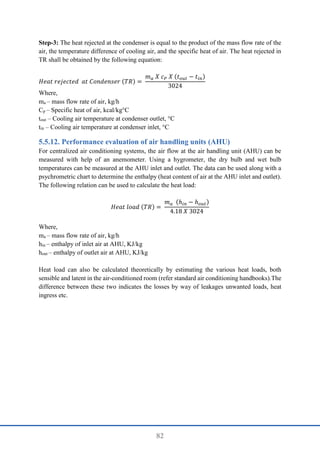
50. 36
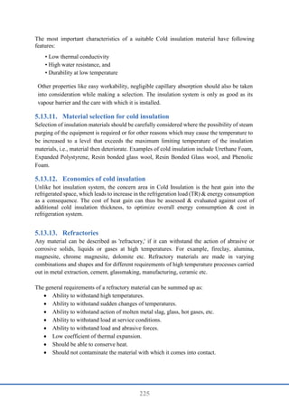
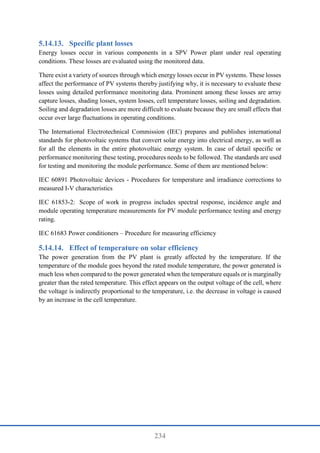
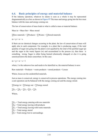
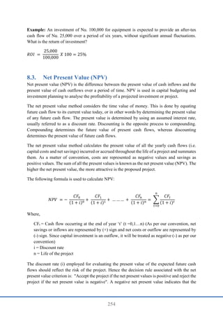
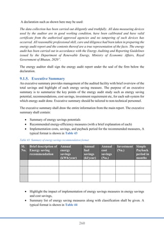
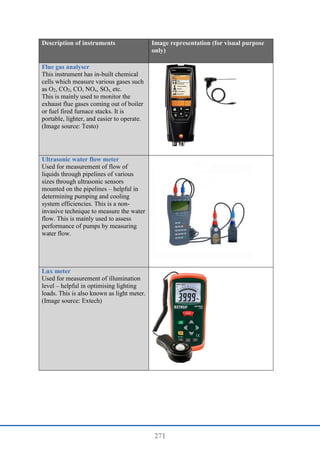
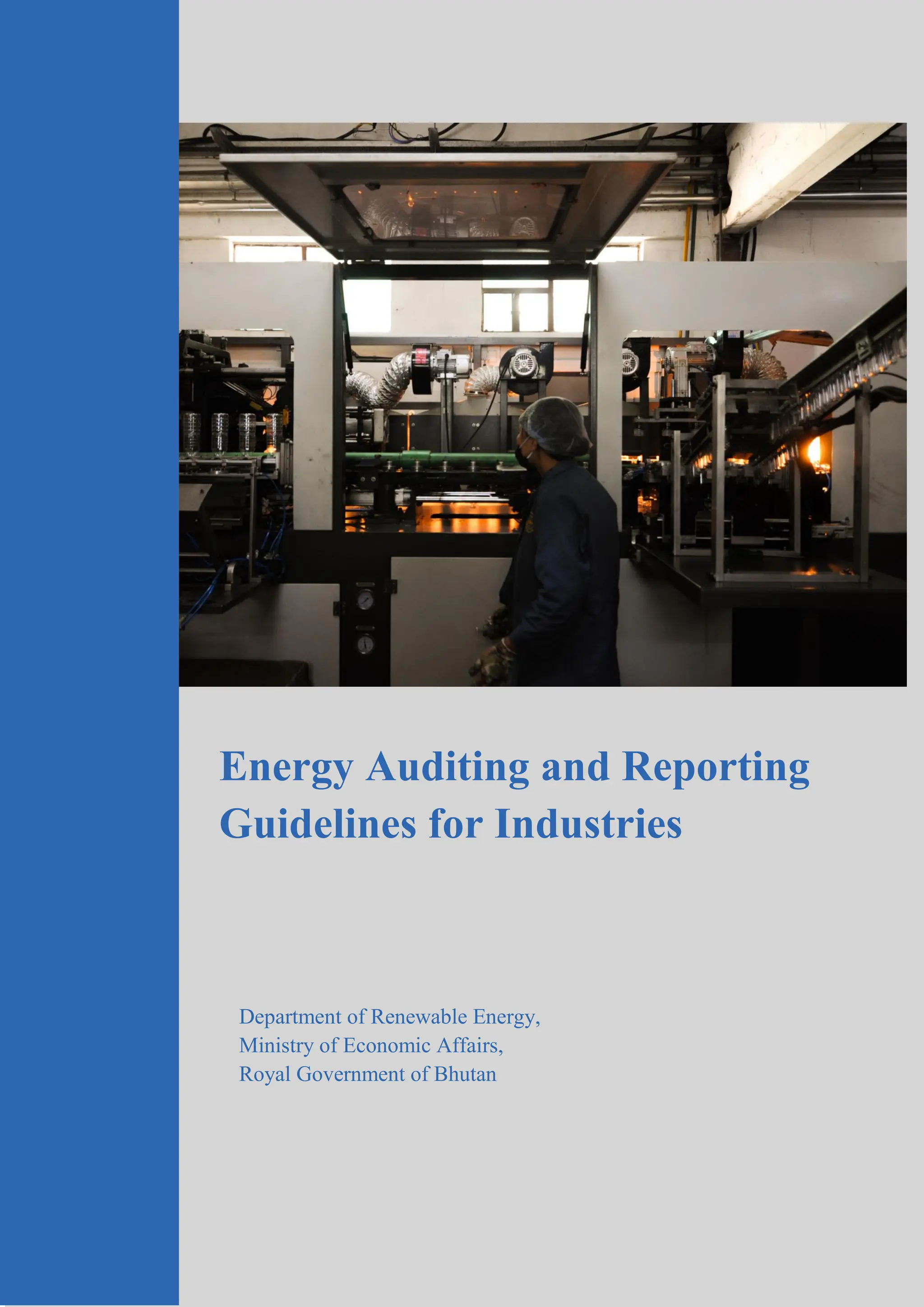
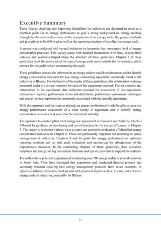
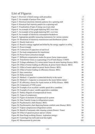
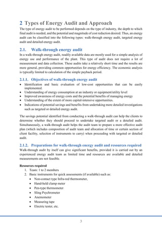
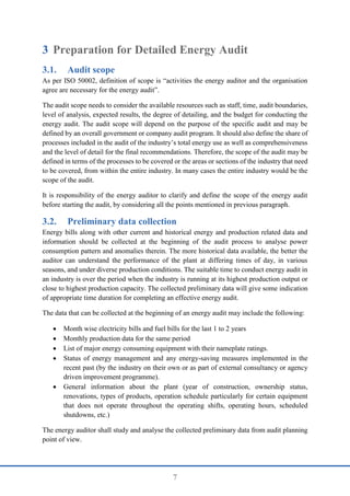
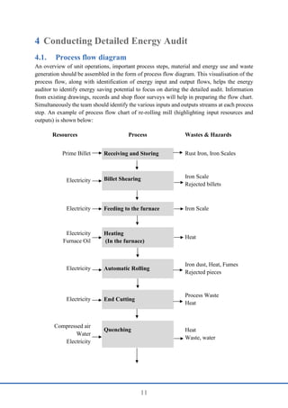
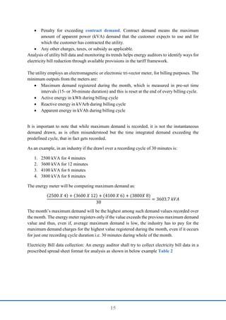
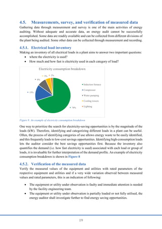
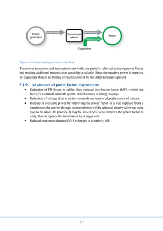
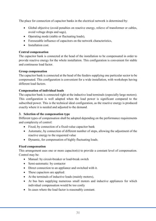
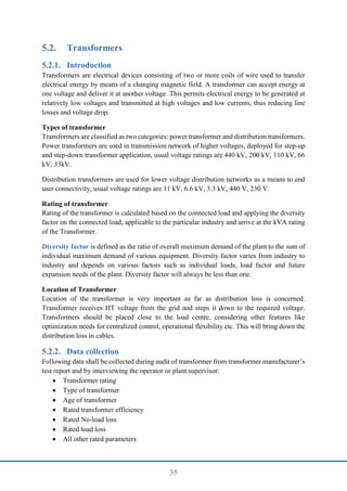
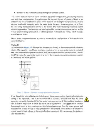
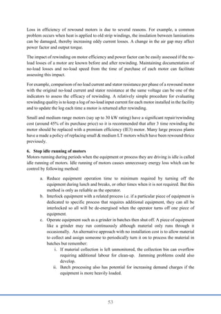
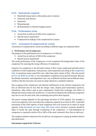
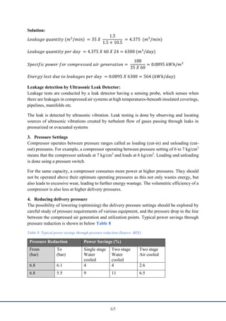
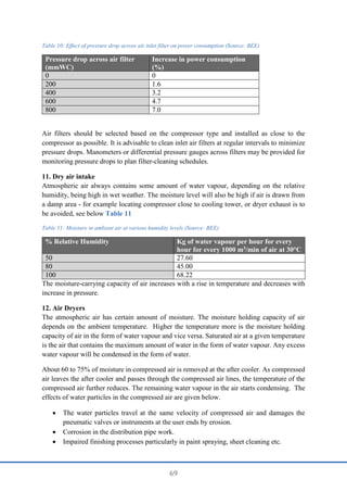
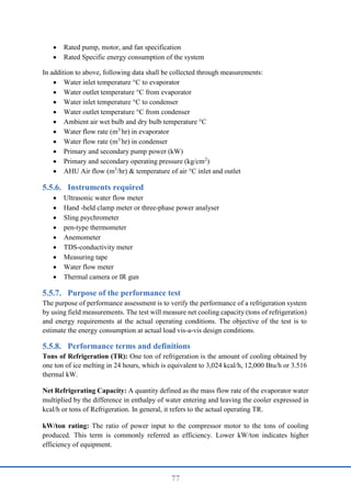
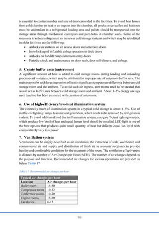
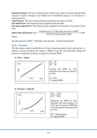
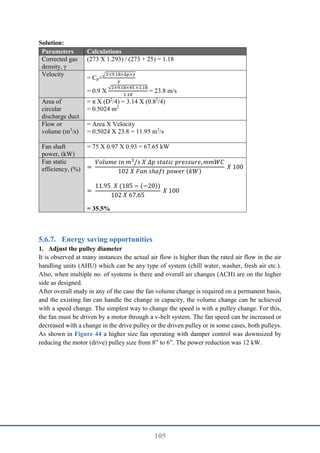
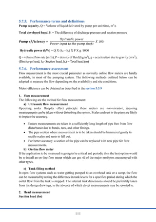
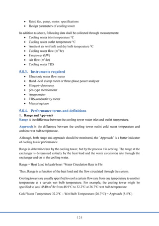
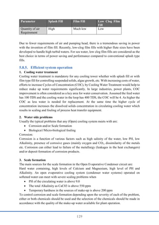
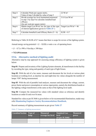
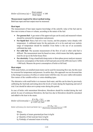
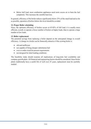
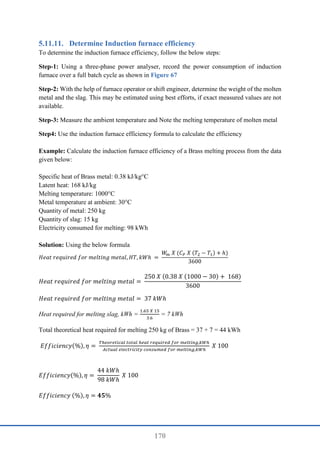
Instruments required
 Three-phase power analyser (2-sets, if applying method-2 to determine transformer
efficiency)
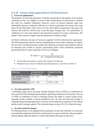
 Thermal imaging camera
Performance terms and definitions
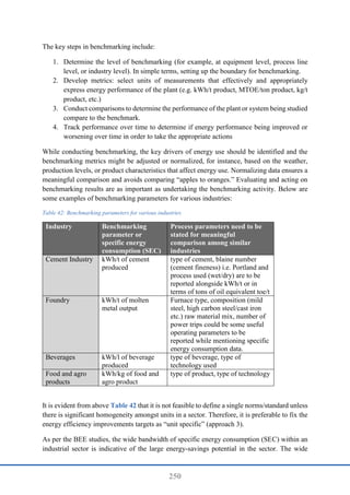
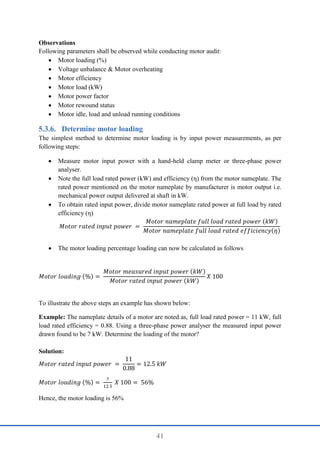
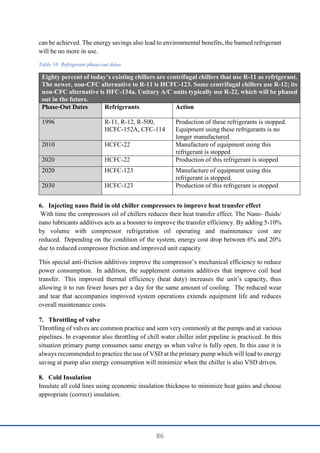
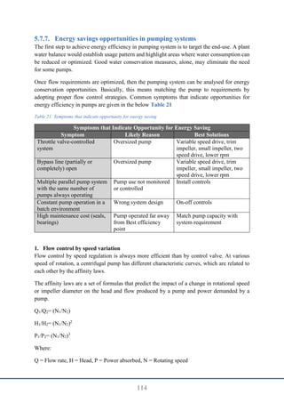
The transformer efficiency varies between 96 to 99%. The efficiency of the transformer
depends on the design of the transformer and the effective operating load.
𝑇𝑟𝑎𝑛𝑠𝑓𝑜𝑟𝑚𝑒𝑟 𝑒𝑓𝑓𝑖𝑐𝑖𝑒𝑛𝑐𝑦 (𝜂) =
𝑂𝑢𝑡𝑝𝑢𝑡 𝑝𝑜𝑤𝑒𝑟
𝑂𝑢𝑡𝑝𝑢𝑡 𝑝𝑜𝑤𝑒𝑟 + 𝑡𝑜𝑡𝑎𝑙 𝑙𝑜𝑠𝑠
𝑋 100
Transformer losses consist of two parts: No-load loss and Load loss
No-load loss also called core loss is the power consumed to sustain the magnetic field in the
transformer’s steel core. Core loss occurs whenever the transformer is energized, core loss does
not vary with load. Core losses are caused by two factors: hysteresis and eddy current losses.
Hysteresis loss is that energy lost by reversing the magnetic field in the core as the magnetizing
AC rises and falls and reverses direction. Eddy current loss is a result of induced currents
circulating in the core.
Load loss (also called copper loss) is associated with full-load current flow in the transformer
windings. Copper loss is power lost in the primary and secondary windings of a transformer
due to the ohmic resistance of the windings. Copper loss varies with the square of the load
current. (P=I2
R).
For a given transformer, the manufacturer can supply values for no-load loss and load loss. The
total transformer loss, at any load level can be calculated from below formula:
Total transformer loss = No load loss + [(Loading (%) of transformer)2
X full load loss]

51. 37
Transformer losses as a percentage of load is given in Figure 18
Figure 18: Transformer losses as a percentage (%) of load (Source: UNEP)
Performance assessment of transformer
Determine transformer efficiency
Method-1
Follow the below steps to determine transformer efficiency:
1. Using a three-phase analyser, measure the average apparent power (kVA) at the
primary side of transformer by CT (current transformer), PT (potential transformer)
ratio conversion method. Caution: Never attach voltage clips directly to primary side
of transformer, it may lead to injury and sudden death.
2. Note the transformer No load loss and load loss from the transformer’s manufacturer
test report which is generally available with facility manager.
3. Also, note the transformer rating from manufacturer test report.
4. Using the below formula, calculate the transformer total loss (kW)
𝑇𝑜𝑡𝑎𝑙 𝑙𝑜𝑠𝑠 (𝑘𝑊) = 𝑁𝑜 𝑙𝑜𝑎𝑑 𝑙𝑜𝑠𝑠 + ((
𝑀𝑒𝑎𝑠𝑢𝑟𝑒𝑑 𝑎𝑝𝑝𝑎𝑟𝑒𝑛𝑡 𝑝𝑜𝑤𝑒𝑟 (𝑘𝑉𝐴)
𝑅𝑎𝑡𝑒𝑑 𝑎𝑝𝑝𝑎𝑟𝑒𝑛𝑡 𝑝𝑜𝑤𝑒𝑟 (𝑘𝑉𝐴)
)
2
𝑋 𝑓𝑢𝑙𝑙 𝑙𝑜𝑎𝑑 𝑙𝑜𝑠𝑠)
5. Using a three-phase power, measure the output power (kW) (at secondary side) of the
transformer.
6. Using the below formula, calculate transformer efficiency
𝑇𝑟𝑎𝑛𝑠𝑓𝑜𝑚𝑒𝑟 𝑒𝑓𝑓𝑖𝑐𝑖𝑒𝑛𝑐𝑦 (𝜂) =
𝑂𝑢𝑡𝑝𝑢𝑡 𝑝𝑜𝑤𝑒𝑟
𝑂𝑢𝑡𝑝𝑢𝑡 𝑝𝑜𝑤𝑒𝑟 + 𝑡𝑜𝑡𝑎𝑙 𝑙𝑜𝑠𝑠
𝑋 100

52. 38
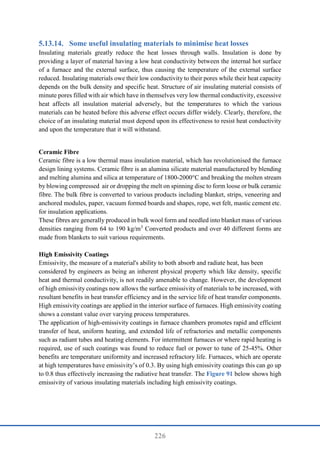
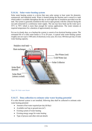
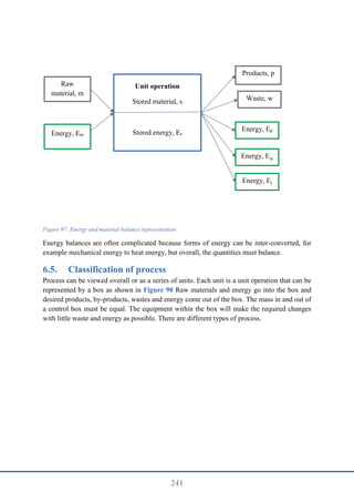
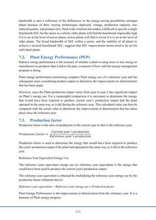
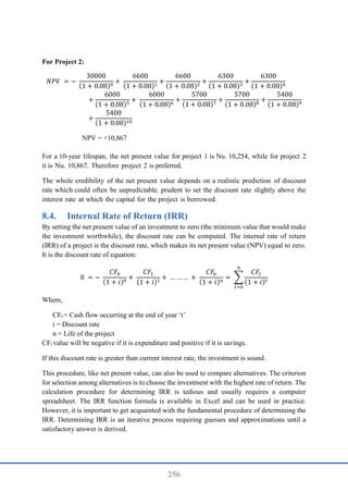
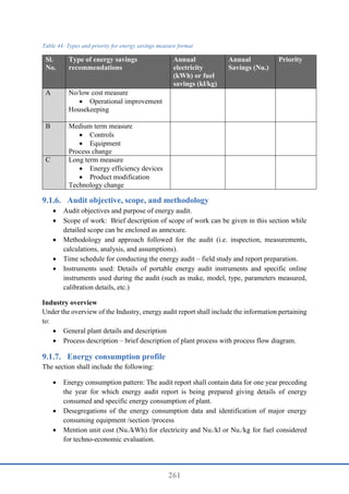
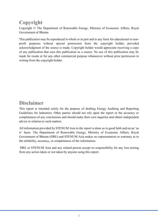
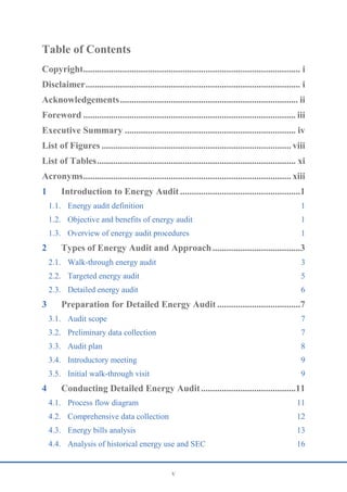
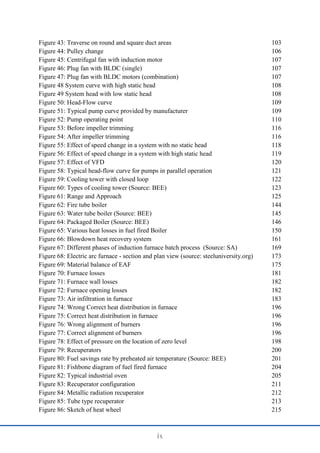
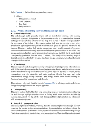
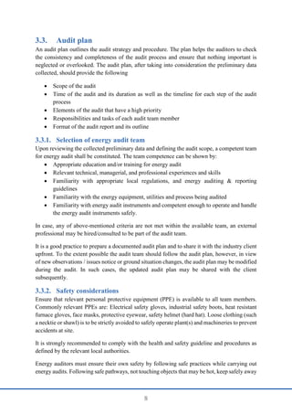
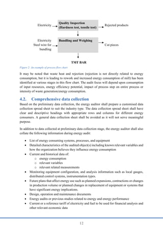
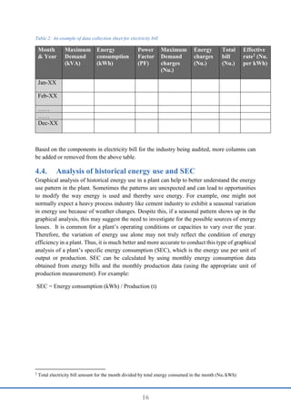
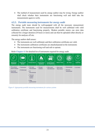
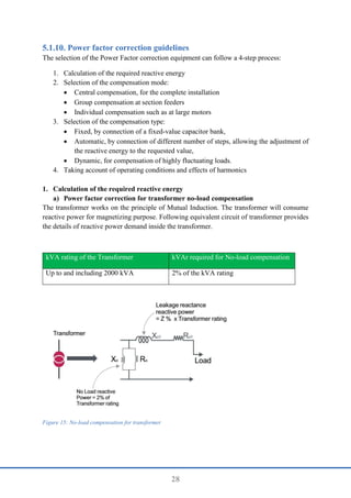
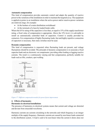
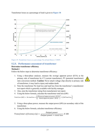
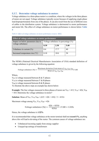
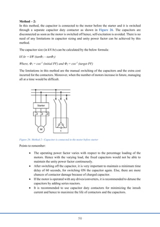
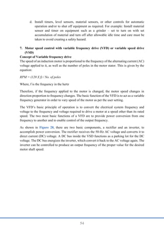
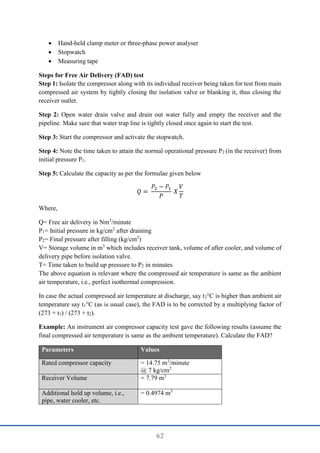
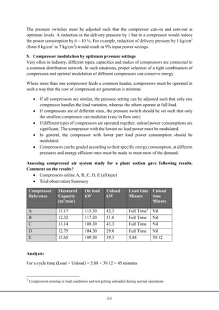
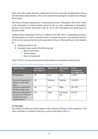
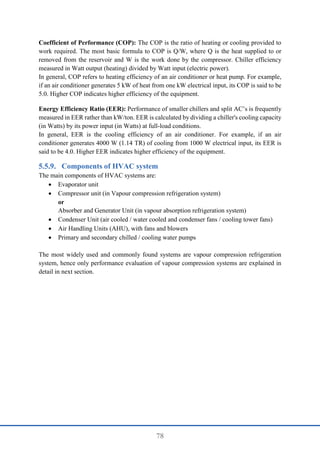
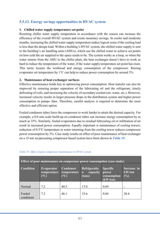
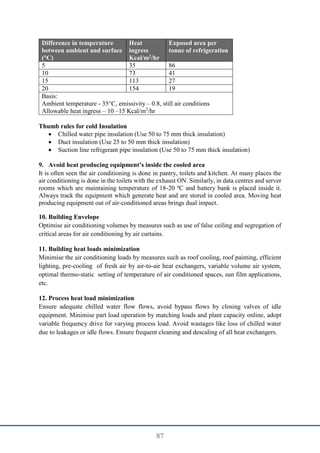
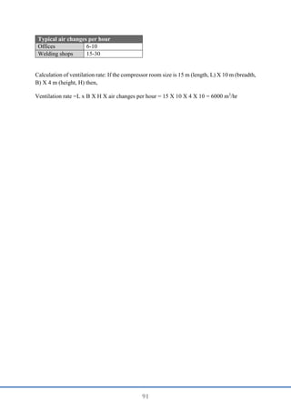
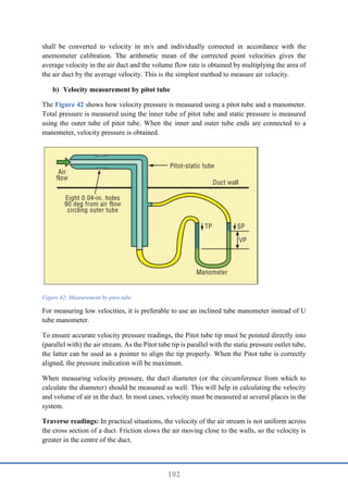
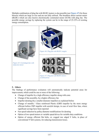
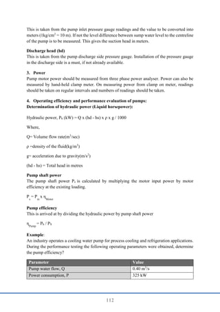
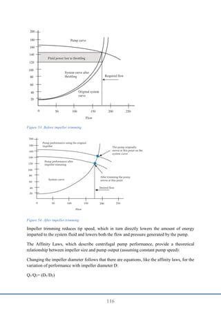
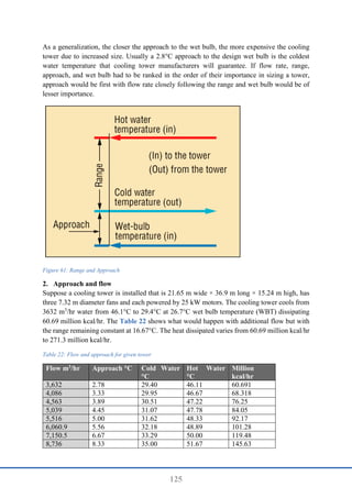
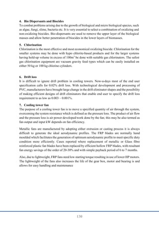
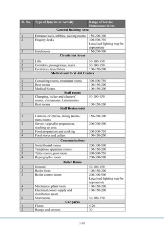
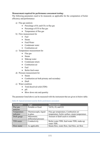
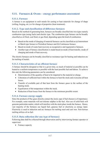
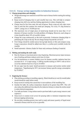
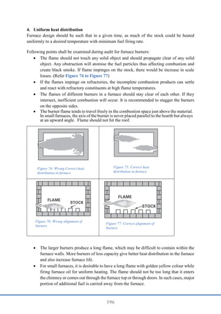
Method-2
1. By using 2 sets of three-phase power analyser, measure simultaneously primary side
input power (kW) and secondary side output power (kW) of transformer.
2. Using the below formula, calculate transformer efficiency
𝑇𝑟𝑎𝑛𝑠𝑓𝑜𝑟𝑚𝑒𝑟 𝑒𝑓𝑓𝑖𝑐𝑖𝑒𝑛𝑐𝑦 (𝜂) =
𝑜𝑢𝑡𝑝𝑢𝑡 𝑝𝑜𝑤𝑒𝑟
𝑖𝑛𝑝𝑢𝑡 𝑝𝑜𝑤𝑒𝑟
𝑋 100
Compare the obtained transformer efficiency with rated efficiency of existing transformer or
new energy efficient transformer. If there is wide variation in efficiencies, use the below
formula to calculate power loss.
Power (kW) loss = Average load (kW) X [(1/ηmeasured – 1/ηrated or new)]
Energy saving opportunity
Replace old (20 years and above) transformers with energy efficient transformers
Most energy loss in dry-type transformers occurs through heat or vibration from the core. The
new high-efficiency transformers minimize these losses. The conventional transformer is made
up of a silicon alloyed iron (grain oriented) core. The iron loss of any transformer depends on
the type of core used in the transformer. However, the latest technology is to use amorphous
material-a metallic glass alloy for the core. The expected reduction in core loss over
conventional (Si Fe core) transformers is roughly around 70%, which is quite significant. By
using an amorphous core- with unique physical and magnetic properties- these new types of
transformers have increased efficiency even at low loads which is 98.5% efficiency at 35%
load. Electrical distribution transformers made with amorphous metal cores provide excellent
opportunity to conserve energy right from the installation.
On a life-cycle cost basis, an energy-efficient transformer is very appealing given its non-stop
operation and 25-year service life. These savings translate into reductions in peak loading,
lower electricity bills and greater reliability of supply. These points should be kept in mind by
the auditor while recommending replacement of inefficient transformers with more efficient
ones. Payback periods vary with the equipment and electricity costs and can be as short as one
year or as long as six years or more. For transformers, a six-year payback on a product that
typically lasts more than 25 years is considered attractive (Source: UNEP)

53. 39
5.3. Motors and application of Variable Frequency Drive (VFD)
Introduction
An electric motor is a device that converts electrical energy into mechanical energy by the
interaction between the magnetic fields set up in the stator and rotor windings. Electric motors
are used in driving a broad range of industrial applications such as pumps, compressors, fans,
blowers, conveyors, and other machines. Motor systems have been identified as being the
major electricity consumer in the industrial sector and the poor efficiency of the substandard
motors leads to more energy consumption and energy cost. Therefore, improvement in
efficiency of the motor must be a part of any comprehensive energy savings effort.
Data collection
Following data shall be collected during audit of motor from motor name plate and by
interviewing the motor operator or plant supervisor:
 Motor manufacturer/make
 Model and type
 Rated motor power (kW)
 Rated motor efficiency and efficiency class
 Rated speed
 All other motor nameplate details
 Motor rewound status (if yes, no. of times rewound)
 Motor operating hours (daily & annual)
 Whether equipped with VFD or not (if yes, note operating frequency and signal
feedback to VFD is manual or automatic)
In addition to above, following data shall be collected through measurements:
 Voltage (V)
 Current (A)
 Power Factor
 Power (kW)
 Motor operating speed (RPM)
 Motor surface temperature
Instruments required
 Hand-held clamp meter
 Three-phase power analyser
 Non-contact type thermometer or thermal imaging camera
 Stroboscope or non-contact type tachometer
 Resistance meter or multi-meter

54. 40
Motor performance terms
Motor efficiency: The efficiency of the motor is given by following relation:
η =
Output power of the motor
Input power of the motor
Motor Loading: The motor loading in percentage (%) is given by following relation:
Motor loading (%) =
Input power drawn by the motor (kW)at existing load
Name plate full load (kW)rating
Name plate full load motor efficiency
𝑋 100
Motor load survey methodology
Large industries have huge numbers of low tension (LT) motors ranging from low rated power
(<1 kW) to high rated power (>200 kW). To identify improvements options a load survey
methodology shall be established as per following factors:
Prioritising motors for audit
The objective of prioritising motor for audit is to select those motors first which are major
energy consumers and representative of all the motors installed in a facility, following criteria
shall be considered for prioritisation:
 Regardless of the motor rated power, preference shall be given to those motors with
continuous running operation or high utilisation factor for example, 18 to 24 hours per
day.
 Motors with high rating power (kW) among the all installed motors shall be given
preference.
 Motors which has been identified as running with inefficient capacity controls on the
machine side or with fluctuating load systems shall be given preference.
 In case, there is a large quantity (>10) of small sized motors in a system (<5 kW) with
same rated power (kW) and due to some constraints measurements on each motor is
not feasible, sample representative method shall be used where measurements and
analysis of one or two motors can be reasoned as representative for all same size motors
in the rest of the system.
Measurements
Studies on motors involves measurement of electrical parameters namely voltage (V), current
(A), power factor (PF), and power drawn (kW) with hand-held clamp meter or three-phase
power analyser without affecting the motor routine operation. Motors running with fluctuating
load shall be chosen for recording the various electrical parameters using three-phase power
analyser over a period as suitable.
Using a non-contact type infra-red thermometer or thermal imaging camera, measure the motor
surface temperature to check motor overheating.

55. 41
Observations
Following parameters shall be observed while conducting motor audit:
 Motor loading (%)
 Voltage unbalance & Motor overheating
 Motor efficiency
 Motor load (kW)
 Motor power factor
 Motor rewound status
 Motor idle, load and unload running conditions
Determine motor loading
The simplest method to determine motor loading is by input power measurements, as per
following steps:
 Measure motor input power with a hand-held clamp meter or three-phase power
analyser.
 Note the full load rated power (kW) and efficiency (η) from the motor nameplate. The
rated power mentioned on the motor nameplate by manufacturer is motor output i.e.
mechanical power output delivered at shaft in kW.
 To obtain rated input power, divide motor nameplate rated power at full load by rated
efficiency (η)
𝑀𝑜𝑡𝑜𝑟 𝑟𝑎𝑡𝑒𝑑 𝑖𝑛𝑝𝑢𝑡 𝑝𝑜𝑤𝑒𝑟 =
𝑀𝑜𝑡𝑜𝑟 𝑛𝑎𝑚𝑒𝑝𝑙𝑎𝑡𝑒 𝑓𝑢𝑙𝑙 𝑙𝑜𝑎𝑑 𝑟𝑎𝑡𝑒𝑑 𝑝𝑜𝑤𝑒𝑟 (𝑘𝑊)
𝑀𝑜𝑡𝑜𝑟 𝑛𝑎𝑚𝑒𝑝𝑙𝑎𝑡𝑒 𝑓𝑢𝑙𝑙 𝑙𝑜𝑎𝑑 𝑟𝑎𝑡𝑒𝑑 𝑒𝑓𝑓𝑖𝑐𝑖𝑒𝑛𝑐𝑦(𝜂)
 The motor loading percentage loading can now be calculated as follows
𝑀𝑜𝑡𝑜𝑟 𝑙𝑜𝑎𝑑𝑖𝑛𝑔 (%) =
𝑀𝑜𝑡𝑜𝑟 𝑚𝑒𝑎𝑠𝑢𝑟𝑒𝑑 𝑖𝑛𝑝𝑢𝑡 𝑝𝑜𝑤𝑒𝑟 (𝑘𝑊)
𝑀𝑜𝑡𝑜𝑟 𝑟𝑎𝑡𝑒𝑑 𝑖𝑛𝑝𝑢𝑡 𝑝𝑜𝑤𝑒𝑟 (𝑘𝑊)
𝑋 100
To illustrate the above steps an example has shown below:
Example: The nameplate details of a motor are noted as, full load rated power = 11 kW, full
load rated efficiency = 0.88. Using a three-phase power analyser the measured input power
drawn found to be 7 kW. Determine the loading of the motor?
Solution:
𝑀𝑜𝑡𝑜𝑟 𝑟𝑎𝑡𝑒𝑑 𝑖𝑛𝑝𝑢𝑡 𝑝𝑜𝑤𝑒𝑟 =
11
0.88
= 12.5 𝑘𝑊
𝑀𝑜𝑡𝑜𝑟 𝑙𝑜𝑎𝑑𝑖𝑛𝑔 (%) =
7
12.5
𝑋 100 = 56%
Hence, the motor loading is 56%

56. 42
Determine voltage unbalance in motors
Voltage unbalance in a three-phase motor is a condition, where the voltages in the three phases
of motor are not equal. Voltage unbalance typically occurs because of supplying single-phase
load disproportionately from one of the phases. It can also result from the use of different sizes
of cables in the distribution system. Voltage unbalance is detrimental to motor performance
and motor life. The effect of voltage unbalance on motor performance is shown below Table
4
Table 4: Effect of voltage unbalance on motor performance (source: BEE)
Effect of voltage unbalance on motor performance
Impact on below parameters due to
voltage unbalance
Voltage unbalance in percentage (%)
0.30 2.30 5.40
Unbalance in current (%) 0.4 17.7 40
Increased temperature rise (°C) 0.18 10.6 58
The NEMA (National Electrical Manufacturers Association of USA) standard definition of
voltage unbalance is given by the following equation:
𝑉𝑜𝑙𝑡𝑎𝑔𝑒 𝑢𝑛𝑏𝑎𝑙𝑎𝑛𝑐𝑒 (%) =
𝑀𝑎𝑥𝑖𝑚𝑢𝑚 𝑑𝑒𝑣𝑖𝑎𝑡𝑖𝑜𝑛 𝑓𝑟𝑜𝑚 𝑚𝑒𝑎𝑛 𝑜𝑓 𝑣𝑅𝑦, 𝑣𝑦𝐵, 𝑣𝐵𝑅
𝑀𝑒𝑎𝑛 𝑜𝑓 𝑣𝑅𝑦, 𝑣𝑦𝐵, 𝑣𝐵𝑅
𝑋 100
Where,
VRY is voltage measured between R & Y phases
VYB is voltage measured between Y & B phases
VBR is voltage measured between B & R phases
To illustrate the above steps an example has shown below:
Example: The line voltages measured in three phases of motor are VRY = 415, VYB = 426, VBR
= 418. Determine the voltage unbalance in motor?
Solution: Mean of VRY, VYB, VBR = (415 + 426 + 418) / 3 = 419.6
Maximum voltage among VRY, VYB, VBR = 426
𝑉𝑜𝑙𝑡𝑎𝑔𝑒 𝑢𝑛𝑏𝑎𝑙𝑎𝑛𝑐𝑒 (%) =
426 − 419.6
419.6
𝑋 100 = 1.52%
Hence, the voltage unbalance is 1.52%
It is recommended that voltage unbalance at the motor terminal shall not exceed 1%, anything
above this will lead to de-rating of the motor. The common causes of voltage unbalance are:
 Unbalanced incoming supply from energy supplier
 Unequal tap settings of transformers

57. 43
 Large single-phase distribution transformer on the system
 Open phase on the primary of a three-phase transformer on the distribution system
 Faults or ground in the power transformer
 Open delta connected transformer banks
 A blown fuse on a three-phase bank of power factor improvement capacitors
 Unequal impedance in conductors of power supply wiring
 Unbalanced distribution of single-phase loads such as lighting
 Heavy reactive single-phase loads such as welders
Voltage unbalance causes overheating of the motor and leading cause of premature failure of
motors. Voltage unbalance causes extremely high current imbalance. The magnitude of current
imbalance may be 6 to 10 times higher as the voltage imbalance. The additional temperature
rise in motors or motor overheating due to voltage unbalance is estimated by following
equation:
Additional temperature rise = 2 X (Voltage unbalance in %)2
For example, if the voltage unbalance is 2% for a motor operating at 100°C, the additional
temperature rise will be 8°C.
The winding insulation life is reduced by one half for each 10°C increase in operating
temperature. The motor losses also increase due to voltage unbalance as shown in Figure 19
Figure 19: Voltage unbalance (%) versus motor losses & motor heating (Source: BEE)

58. 44
Motor Efficiency
Two important attributes relating to efficiency of electricity use by A.C. inductionmotors are
efficiency (η), defined as the ratio of the mechanical energy delivered at the rotating shaft to
the electrical energy input at its terminals, and power factor (PF). Motors, like other inductive
loads, are characterized by power factors less than one. As a result, the total current draw
needed to deliver the same real power is higher than for a load characterized by a higher PF.
An important effect of operating with a PF less than one is that resistance losses in wiring
upstream of the motor will be higher since these are proportional to the square of the
current. Thus, both a high value for η and a PF close to unity are desired for efficient overall
operation in a plant.
Squirrel cage motors are normally more efficient than slip-ring motors, and higher-speed
motors are normally more efficient than lower-speed motors. Efficiency is also a function of
motor temperature. Totally enclosed fan-cooled (TEFC) motors are more efficient than
screen-protected, drip-proof (SPDP) motors. Also, as with most equipment, motor efficiency
increases with the rated capacity.
The efficiency of a motor is determined by intrinsic losses that can be reduced only by
changes in motor design. Intrinsic losses are of two types: fixed losses- independent of motor
load, and variable losses - dependent on load.
Fixed losses consist of magnetic core losses and friction and windage losses. Magnetic
core losses (sometimes called iron losses) consist of eddy current and hysteresis losses in
the stator. They vary with the core material and geometry and with input voltage. Friction
and windage losses are caused by friction in the bearings of the motor and aerodynamic losses
associated with the ventilation fan and other rotating parts.
Variable losses consist of resistance losses in the stator and in the rotor and miscellaneous
stray losses. Resistance to current flow in the stator and rotor result in heat generation, that is
proportional to the resistance of the material and the square of the current (I2
R). Stray losses
arise from a variety of sources and are difficult to either measure directly or to calculate but
are generally proportional to the square of the rotor current. Part load performance
characteristics of a motor also depend on its design. Both the η and PF fall to very low levels
at low load. Figure 20 shows the effect of load on power factor and efficiency. Power factor
drops sharply at part loads. Figure 21 shows the effect of speed on power factor.

59. 45
Figure 20: Effect of motor loading on efficiency & power factor (Source: BEE)
Figure 21: Effect of motor speed on power factor (Source: BEE)

60. 46
Determine motor efficiency
The efficiency of induction motors remains almost constant between 50% to 100% loading
(refer, Figure 22) hence for simplicity motor nameplate efficiency rating may be used for
calculations if the motor is operating in the range of 50 to 100% loading.
However, the following method can be also used to determine the motor efficiency.
Step-1: Perform the following actions under no load conditions
 Using a resistance meter, measure stator resistance at ambient temperature.
 Run the motor at rated voltage and frequency without any shaft load
 Using a hand-held clamp meter or three-phase power analyser, measure the power
(Watts) and current.
 Calculate the iron plus friction and windage loss using below formula
 Iron plus friction and windage loss (Watts) =No load power (Watts) - (no load current)2
X Stator resistance
Step-2: Perform the following actions under load conditions
 Run the motor at rated voltage and frequency with full load
 Using a hand-held clamp meter or three-phase power analyser, measure the power
(Watts) and current
 Using a non-contact type infra-red thermometer, measure operating temperature of
motor
 The stator resistance measured at ambient temperature must be corrected for the
operating temperature. The correction factor is as follows:
𝑅𝑜𝑝𝑒𝑟𝑎𝑡𝑖𝑛𝑔 = 𝑅𝑎𝑚𝑏𝑖𝑒𝑛𝑡 𝑋
235 + 𝑜𝑝𝑒𝑟𝑎𝑡𝑖𝑛𝑔 𝑡𝑒𝑚𝑝𝑒𝑟𝑎𝑡𝑢𝑟𝑒
235 + 𝑎𝑚𝑏𝑖𝑒𝑛𝑡 𝑡𝑒𝑚𝑝𝑒𝑟𝑎𝑡𝑢𝑟𝑒
Figure 22: Effect of motor loading on efficiency (Source: BEE)

61. 47
Where,
Roperating is resistance corrected for operating temperature
Rambient is resistance measured at ambient temperature
 Calculate the stator copper loss at full load using below formula
Stator copper loss at full load (Watts) = I² (full load current) X Roperating
Step-3: Calculate the rotor power
 Run the motor at rated voltage and frequency with full load
 Using a stroboscope or non-contact type tachometer, measure the speed of the motor in
RPM (revolutions per minute) at full load.
 Calculate slip by using below formula. Where, synchronous speed is the motor
nameplated rated speed
𝑆𝑙𝑖𝑝 (𝑆) =
𝑆𝑦𝑛𝑐ℎ𝑟𝑜𝑛𝑜𝑢𝑠 𝑠𝑝𝑒𝑒𝑑 − 𝑓𝑢𝑙𝑙 𝑙𝑜𝑎𝑑 𝑠𝑝𝑒𝑒𝑑
𝑆𝑦𝑛𝑐ℎ𝑟𝑜𝑛𝑜𝑢𝑠 𝑠𝑝𝑒𝑒𝑑
 Calculate rotor power using below formula
𝑅𝑜𝑡𝑜𝑟 𝑝𝑜𝑤𝑒𝑟 (𝑊𝑎𝑡𝑡𝑠) =
𝑀𝑜𝑡𝑜𝑟 𝑛𝑎𝑚𝑒𝑝𝑙𝑎𝑡𝑒 𝑟𝑎𝑡𝑒𝑑 𝑝𝑜𝑤𝑒𝑟
1 − 𝑆𝑙𝑖𝑝
Step-4: Calculate motor full load input power
 Use the below formula to calculate the motor full load input power
Motor full load input power = Iron plus windage and friction loss + Stator copper loss at
full load + Rotor power + Stray losses
 Use the below Table 5 adapted from IEEE for stray losses as measurement of stray
losses is a complicated process which is not possible on shop floor.
Table 5: Motor rating versus stray losses (adapted from IEEE)
Motor rating Stray losses
0.75 – 93 kW 1.8%
93 – 373 kW 1.5%
373 – 1863 kW 1.2%
1864 and above 0.9%
Step-5: Calculate motor efficiency
 Use the below formula to calculate the motor efficiency
𝑀𝑜𝑡𝑜𝑟 𝑒𝑓𝑓𝑖𝑐𝑖𝑒𝑛𝑐𝑦 (𝜂) =
𝑀𝑜𝑡𝑜𝑟 𝑛𝑎𝑚𝑒𝑝𝑙𝑎𝑡𝑒 𝑟𝑎𝑡𝑒𝑑 𝑝𝑜𝑤𝑒𝑟
𝑀𝑜𝑡𝑜𝑟 𝑓𝑢𝑙𝑙 𝑙𝑜𝑎𝑑 𝑖𝑛𝑝𝑢𝑡 𝑝𝑜𝑤𝑒𝑟

62. 48
Energy savings opportunities in motor
1. Improve motor loading
For motors, which consistently operate at loads below 40% of rated capacity, an inexpensive
and effective measure is to operate in star mode.
A change from the standard delta operation to permanent star operation involves re-configuring
the wiring at terminal box and resetting of the
over-current relay. Operating in the star mode leads to a voltage reduction by a factor of ‘√3’.
Motor is electrically downsized by one-third (1/3rd
) in star mode operation, but performance
characteristics as a function of load remain unchanged. For example, if a motor is rated for 15
kW in delta mode, its de-rated capacity is 5kW in star mode. Thus, full-load operation in star
mode gives higher efficiency and power factor than partial load operation in the delta mode.
However, motor operation in the star mode is possible only for applications where the torque-
to-speed requirement is lower at reduced load.
As speed of the motor reduces in star mode this option may be avoided in case the motor is
connected to a production facility whose output is related to the motor speed. Further, in star
mode the motor loading should not be allowed to cross de-rated capacity. For example, in
above case of 15 kW delta connected electric motor, should not be loaded above 5 kW when
delta to star switchover takes place.
For applications with high initial torque and low running torque needs, automatic Star-Delta-
Star converters are also available, which help in load following de-rating of electric motors
after initial start-up.
2. Motor power factor (PF) correction
Induction motors which operate at power factors less than unity, leads to lower overall
efficiency and higher overall operating cost associated with a facility's electrical system.
Capacitors connected in parallel (shunted) with the motor are typically used to improve the
power factor. The benefits of PF correction are as below:
 Reduced apparent power (kVA) demand and hence reduced utility demand charges.
 Reduced copper losses (I2
R) in cables upstream of the capacitor and hence reduced
energy charges.
 Reduced voltage drop in the cables leading to improved voltage regulation.
Figure 23: Star connection Figure 24: Delta connection

63. 49
 Increase in the overall efficiency of the plant electrical system.
The various methods of power factor correction are central compensation, group compensation
and individual compensation. Depending upon the size and the rate of change of loads in an
industry, any one or combination of the above methods can be employed. Specifically, in case
of some small-scale industries with a few motor loads, the power factor correction can be done
by connecting shunt capacitors directly to the motors. This method of compensation is called
direct compensation. This is simple and ideal method for reactive power compensation, as this
would result in rating optimization of all the upstream switchgear and cables, which reduces
overall system losses.
Direct motor compensation can be done in two methods, configuration of both methods is
described below:
Method-1
As shown in the Figure 25, the capacitor is connected directly to the motor terminals, after the
starter. The capacitors would start supplying reactive power as soon as the motor is switched
ON. This method of compensation can be used for motors with direct online starters. Usually
the kVAr rating for a particular motor is given by the respective motor manufacturers, as the
kVAr ratings are motor specific.
Even though this is the effective method of power factor compensation, there is a limitation in
sizing of the capacitors. That is, the maximum kVAr should be decided such that, the rated
capacitor current is less than 90% of the motor’s no-load current. If this condition is not met,
self-excitation may occur, in which the motor acts as a generator. This happens when a motor
has enough inertia to keep rotating even after being disconnected from the power system and
the capacitor is large enough to supply the reactive power needs of the motor. Self-excitation
would result in high voltage at the terminals of the motor and this can damage the contactor
and the capacitor.
Figure 25: Method 1- Capacitor is connected directly to the motor

64. 50
Method – 2:
In this method, the capacitor is connected to the motor before the starter and it is switched
through a separate capacitor duty contactor as shown in Figure 26. The capacitors are
disconnected as soon as the motor is switched off hence, self-excitation is avoided. There is no
need of any limitations in capacitor sizing and unity power factor can be achieved by this
method.
The capacitor size (in kVAr) can be calculated by the below formula:
kVAr = kW (tanΦ1 – tanΦ2)
Where, Φ1 = cos-1
(initial PF) and Φ2 = cos-1
(target PF)
The limitations in this method are the manual switching of the capacitors and the extra cost
incurred for the contactors. Moreover, when the number of motors increase in future, managing
all at a time would be difficult.
Figure 26: Method 2 - Capacitor is connected to the motor before starter
Points to remember:
 The operating power factor varies with respect to the percentage loading of the
motors. Hence with the varying load, the fixed capacitors would not be able to
maintain the unity power factor continuously.
 After switching off the capacitor, it is very important to maintain a minimum time
delay of 60 seconds, for switching ON the capacitor again. Else, there are more
chances of contactor damage because of charged capacitor.
 If the motor is operated with any drives/converters, it is recommended to detune the
capacitors by adding series reactors.
 It is recommended to use capacitor duty contactors for minimizing the inrush
current and hence to maximize the life of contactors and the capacitors.

65. 51
3. Energy efficient motor technical characteristics
The IEC (International Electrotechnical Commission) has contributed to the development of
energy efficient electric motor systems through the internationally relevant test standard IEC
60034-2-1 for electric motors and the IEC 60034-30-1 classification scheme comprising four
levels of motor efficiency:
 IE1 Standard Efficiency
 IE2 High Efficiency
 IE3 Premium Efficiency
 IE4 Super premium Efficiency
Acknowledging the need for energy saving in view of the energy scarcity, climate change
mitigations and the potential that exists with energy efficient motors, number of countries have
issued directives to withdraw lower efficiency classes and adopt higher efficiency class motors
as per IEC 60034-30-1: 2014, thus defining minimum efficiency performance standards
(MEPS) in their countries. Such regulations are expected to impose technical barriers to all the
imports of motors which are with lower efficiency classes than the MEPS into their countries.
The European Union sets motor MEPS levels at IE3 (or IE2 in combination with VFD) from
2017 covering motors with 0.75 kW up to 375 kW. In 2018, India also sets efficiency class IE2
as Minimum Energy Performance Standard (MEPS) for LT motors.
Figure 27: IE efficiency classes for 4 pole motors at 50 Hz (Source: ABB)

66. 52
4. Cost effectiveness of energy efficient motors
The energy savings by motor replacement can be worked out by a simple formula:
𝑃𝑜𝑤𝑒𝑟 𝑠𝑎𝑣𝑖𝑛𝑔𝑠 (𝑘𝑊) = 𝑃𝑜𝑤𝑒𝑟 𝑜𝑢𝑡𝑝𝑢𝑡 (𝑘𝑊) 𝑋
1
𝜂𝑜𝑙𝑑
−
1
𝜂𝑛𝑒𝑤
Where, 𝜂𝑜𝑙𝑑 is efficiency of the existing old motor
Where, 𝜂𝑛𝑒𝑤 is efficiency of the proposed new motor
Annual energy savings = Power savings (kW) X annual operating hours of the motor
To illustrate the above formula, an example has shown below:
Example: During an energy audit following data were obtained on a 3-phase induction motor:
Rated values: 37 kW, 415 V, 66 A, PF = 0.88, η = 0.88
Measured values: 410 V, 49 A, PF = 0.76 pf, P = 26.44 kW
The plant operates for 7000 hours per year, and it is proposed to replace the existing motor by
a 30 kW, new energy efficient motor with rated efficiency of 92%.
a) Determine loading% of the existing motor.
b) Determine the energy savings with new energy efficient motor
Solution: Rated input power of the motor = Rated power / efficiency (η)
Parameters Calculations
Rated input power of the existing
motor at full load
= 37 / 0.88 = 42 kW
Loading of the existing motor = measured power / rated input power
= 26.44 / 42 = 63%
Shaft power or motor output of the
existing motor
= 37 X 63% =23.31 kW
New energy efficient motor rating = 30 kW
Actual shaft power or motor output
required
= 23.31 kW
Loading% of new energy efficient
motor
= 23.31 / 30 = 77.7%
Power savings = 23.31 (1/0.88 – 1/0.92) = 1.16 kW
Annual energy savings = 1.16 X 7000 = 8,120 kWh
Points to be noted: Though the new energy efficient motor is of 30 kW, but the energy savings
will be calculated at the actual shaft power delivered by the motor or the motor output required.
5. Motor rewinding effects on energy efficiency
It is common practice in industry to rewind burnt-out motors. Careful rewinding may
sometimes maintain motor efficiency at previous levels, but in most cases rewinding results in
efficiency loss.

67. 53
Loss in efficiency of rewound motors is due to several reasons. For example, a common
problem occurs when heat is applied to old strip windings, the insulation between laminations
can be damaged, thereby increasing eddy current losses. A change in the air gap may affect
power factor and output torque.
The impact of rewinding on motor efficiency and power factor can be easily assessed if the no-
load losses of a motor are known before and after rewinding. Maintaining documentation of
no-load losses and no-load speed from the time of purchase of each motor can facilitate
assessing this impact.
For example, comparison of no load current and stator resistance per phase of a rewound motor
with the original no-load current and stator resistance at the same voltage can be one of the
indicators to assess the efficacy of rewinding. A relatively simple procedure for evaluating
rewinding quality is to keep a log of no-load input current for each motor installed in the facility
and to update the log each time a motor is returned after rewinding.
Small and medium range motors (say up to 30 kW rating) have a significant repair/rewinding
cost (around 45% of its purchase price) so it is recommended that after 3 time rewinding the
motor should be replaced with a premium efficiency (IE3) motor. Many large process plants
have a made a policy of replacing small & medium LT motors which have been rewound thrice
previously.
6. Stop idle running of motors
Motors running during periods when the equipment or process they are driving is idle is called
idle running of motors. Idle running of motors causes unnecessary energy loss which can be
control by following method:
a. Reduce equipment operation time to minimum required by turning off the
equipment during lunch and breaks, or other times when it is not required. But this
method is only as reliable as the operator.
b. Interlock equipment with a related process i.e. if a particular piece of equipment is
dedicated to specific process that requires additional equipment, they can all be
interlocked so all will be de-energised when the operator turns off one piece of
equipment.
c. Operate equipment such as a grinder in batches then shut off. A piece of equipment
like a grinder may run continuously although material only runs through it
occasionally. An alternative approach with no installation cost is to allow material
to collect and assign someone to periodically turn it on to process the material in
batches but remember:
i. If material collection is left unmonitored, the collection bin can overflow
requiring additional labour for clean-up. Jamming problems could also
develop.
ii. Batch processing also has potential for increasing demand charges if the
equipment is more heavily loaded.

68. 54
d. Install timers, level sensors, material sensors, or other controls for automatic
operation and/or to shut off equipment as required. For example: Install material
sensor and timer on equipment such as a grinder – set to turn on with set
accumulation of material and turn off after allowable idle time and care must be
taken to avoid creating a safety hazard.
7. Motor speed control with variable frequency drive (VFD) or variable speed drive
(VSD)
Concept of Variable frequency drive
The speed of an induction motor is proportional to the frequency of the alternating current (AC)
voltage applied to it, as well as the number of poles in the motor stator. This is given by the
equation:
RPM = (120 X f) / No. of poles
Where, f is the frequency in the hertz
Therefore, if the frequency applied to the motor is changed, the motor speed changes in
direction proportion to frequency changes. The basic function of the VFD is to act as a variable
frequency generator in order to vary speed of the motor as per the user setting.
The VFD’s basic principle of operation is to convert the electrical system frequency and
voltage to the frequency and voltage required to drive a motor at a speed other than its rated
speed. The two most basic functions of a VFD are to provide power conversion from one
frequency to another and to enable control of the output frequency.
As shown in Figure 28, there are two basic components, a rectifier and an inverter, to
accomplish power conversion. The rectifier receives the 50-Hz AC voltage and converts it to
direct current (DC) voltage. A DC bus inside the VSD functions as a parking lot for the DC
voltage. The DC bus energizes the inverter, which convert it back to the AC voltage again. The
inverter can be controlled to produce an output frequency of the proper value for the desired
motor shaft speed.

69. 55
In many applications, the input power is a function of the speed like fan, blower, pump,
conveyor and so on. In these types of loads, the torque is proportional to the square of the speed
and the power is proportional to the cube of speed.
Power α (speed)3
Variable speed, depending upon the load requirement, provides significant energy saving. A
reduction of 20% in the operating speed of the motor from its rated speed will result in an
almost 50% reduction in the input power to the motor. This is not possible in a system where
the motor is directly connected to the supply line. In many flow control applications, a
mechanical throttling device is used to limit the flow. Although this is an effective means of
control, it wastes energy because of the high losses and reduces the life of the motor valve due
to generated heat.
Factors for successful implementation of variable frequency drives
a) Understanding load type for Variable Frequency Drives
The main consideration is whether the variable frequency drive application requires a variable
torque or constant torque drive. If the equipment being driven is centrifugal, such as a fan or
pump, then a variable torque drive will be more appropriate. Energy savings are usually the
primary motivation for installing variable torque drives for centrifugal applications. For
example, a fan needs less torque when running at 50% speed than it does when running at full
speed. Variable torque operation allows the motor to apply only the torque needed, which
results in reduced energy consumption.
Conveyors, positive displacement pumps, punch presses, extruders, and other similar type
applications require constant level of torque at all speeds. In which case, constant torque
variable frequency drives would be more appropriate for the job. A constant torque drive
should have an overload current capacity of 150% or more for one minute. Variable torque
variable frequency drives need only an overload current capacity of 120% for one minute since
centrifugal applications rarely exceed the rated current.
Figure 28: Component of VFD system

70. 56
b) Collecting motor information
The following motor information will be needed to select the proper variable frequency drive:
Full load current rating: Using a motor's power rating is an unreliable way to size variable
frequency drives. Full load current rating of the motor shall be considered to estimate VFD
size.
Speed range: Generally, a motor should not be run at any speed less than 20% of its specified
maximum speed allowed. If it is run at a speed less than this without auxiliary motor cooling,
the motor will overheat. Auxiliary motor cooling should be used if the motor must be operated
at very slow speeds.
Multiple motors: To size a variable frequency drive that will control more than one motor,
add together the full load current ratings of each of the motors. All motors controlled by a
single drive must have an equal voltage rating.
c) Efficiency and power factor of VFD
The variable frequency drive should have an efficiency rating of 95% or more at full load.
Variable frequency drives should also offer a true system power factor of 0.95 or more across
the operational speed range, to save on demand charges, and to protect the equipment
(especially motors).
d) Protection circuits for VFD
Motor overload Protection for instantaneous trip and motor over current should be provided.
Additional protection circuits shall also be provided for over and under voltage, over
temperature, ground fault, control or microprocessor fault. These protective circuits should
provide an orderly shutdown of the VFD, provide indication of the fault condition, and require
a manual reset (except under voltage) before restart. Under voltage from a power loss shall be
set to automatically restart after return to normal. The history of the previous three faults shall
remain in memory for future review.
e) Selection of equipment for VFD operation
The first step is to identify the operating hours of the equipment at various load conditions.
This can be done using a power analyser with continuous data storage or by a simple energy
meter with periodic reading being taken.
To determine if the equipment under consideration is the right choice for a variable speed drive,
the load patterns should be thoroughly studied before exercising the option of VFD. In effect
the load should be of a varying nature to demand a VFD

71. 57
0
5
10
15
20
25
30 35 40 45 50 55 60 65 70 75 80 85 90 95 100
Percent
Operating
Hours
Percent Rated Flow
Figure 29: Example of an excellent variable speed drive candidate
0
5
10
15
20
25
30 35 40 45 50 55 60 65 70 75 80 85 90 95 100
Percent
Operating
Hours
Percent Rated Flow
Figure 30: Example of a poor variable speed drive candidate

72. 58
5.4. Air Compressors – energy performance assessment
Introduction
Air compressors account for significant amount of electricity used in industries. In fact, over
the lifespan of a typical compressor, energy typically costs several times more than the
purchase price of the compressor. Air compressors are used in a variety of industries to supply
process requirements, to operate pneumatic tools and equipment, and to meet instrumentation
needs. Only 10~30% of energy reaches the point of end-use, and balance 70~90% of energy of
the power of the prime mover being converted to unusable heat energy and to a lesser extent
lost in form of friction, misuse and noise.
Types of Compressor
Compressors are broadly classified as:
 Positive displacement compressor: Positive displacement compressors increase the
pressure of the gas by reducing the volume. Positive displacement compressors are
further classified as reciprocating and rotary compressors.
 Dynamic compressor: Dynamic compressors increase the air velocity, which is then
converted to increased pressure at the outlet. Dynamic compressors are basically
centrifugal compressors and are further classified as radial and axial flow types.
The flow and pressure requirements of a given application determine the suitability of a type
of compressor.
Figure 31: Sankey diagram of compressed air losses

73. 59
Figure 32: Types of compressors
Data collection
1. Following data shall be collected during audit of compressor from compressor name
plate and by interviewing the motor operator or plant supervisor:
 Compressor make
 Type of compressor- Reciprocating/Screw/Centrifugal/Other
 Sub type- Lubricated/Non lubricated/Air cooled/water cooled
 Model of compressor
 Rated Free air delivery (cfm or m3
/min or m3
/hr)
 Rated power
 Rated specific power consumption
 Rated motor speed (RPM)
 Cut-in and cut-off pressure
While collecting information, it should also be checked, whether the compressors are installed
with variable speed drive, synthetic flat belt, pressure controllers, auto cut off valves or any
other energy saving retrofits.
2. Details of compressed air network
The compressed air network diagram should be collected or made depicting the major
compressed air consuming equipment. It is necessary to collect the pressurized air requirement
and information pertaining to the major users as shown in Table 6
Compressor Types
Positive Displacement
Reciprocating Rotary
Lobe
Liquid Ring
Screw
Vane
Dynamic
Centrifugal Axial
Single-acting
Double-acting
Diaphragm

74. 60
Table 6: Equipment wise compressed air requirement
Equipment Section Compressed air
pressure
requirement
kg/cm2
Compressed air
requirement,
CFM or m3/min
Application
3. Details of air dryer installed
4. Schematic diagram of compressed air network
Elements of compressed air system:
Following Figure 33 shows different elements of compressed air system.
Figure 33: Figure of elements of compressed air system showing generation, distribution, and usage (Source:
Gison Pneumatics)
As shown in the above Figure 33 Compressed air system in any industry can be divided into
three stages of
A. Generation
B. Distribution
C. Usage
While look for energy saving option in compressed air system, assessment should also follow
the same stages of system.

75. 61
Instruments required
 Hand-held clamp meter or three-phase power analyser
 Ultrasonic leak detector
 Stopwatch
 Measuring tape
 IR thermometer or thermal imaging camera
Performance terms
 Actual free air delivery (FAD) of the compressor
 Specific power requirement
 Compressed air leakage in the compressed air systems
Assessment of compressed air system:
Assessment of compressed air system according to different stages are explained below:
1. Performance test of compressor
The purpose of the performance test of compressor is to find out:
• Actual free air delivery (FAD) of the compressor
• Specific power requirement
The actual performance of the compressor is to be compared with design/rated values of the
compressor for assessing the energy efficiency of compressor.
Capacity of a compressor is the full rated volume of flow of gas compressed and delivered at
conditions of total temperature, total pressure, and composition prevailing at the compressor
inlet. It sometimes means actual flow rate, rather than rated volume of flow. This also termed
as Free Air Delivery (FAD) i.e. air at atmospheric conditions at any specific location. Because
the altitude, barometer, and temperature may vary at different localities and at different times,
it follows that this term does not mean air under identical or standard conditions.
Due to ageing of the compressors and inherent inefficiencies in the internal components, the
free air delivered may be less than the design value, despite good maintenance practices.
Sometimes, other factors such as poor maintenance, fouled heat exchanger and effects of
altitude also tend to reduce free air delivery. To meet the air demand, the inefficient compressor
may have to run for more time, thus consuming more power than required.
The power wastage depends on the percentage deviation of FAD capacity. For example, a
worn-out compressor valve can reduce the compressor capacity by as much as 20%. A periodic
assessment of the FAD capacity of each compressor has to be carried out to check its actual
capacity. If the deviations are more than 10% from rated, corrective measures should be
taken to rectify the same through overhauling of the compressor. A well-maintained air
compressor is expected to deliver 90 to 100% of the rated volumetric flow (free air delivery).
The simplest method to determine free air delivery of compressor is pump up method which is
described below.
Instruments required for FAD test:

76. 62
 Hand-held clamp meter or three-phase power analyser
 Stopwatch
 Measuring tape
Steps for Free Air Delivery (FAD) test
Step 1: Isolate the compressor along with its individual receiver being taken for test from main
compressed air system by tightly closing the isolation valve or blanking it, thus closing the
receiver outlet.
Step 2: Open water drain valve and drain out water fully and empty the receiver and the
pipeline. Make sure that water trap line is tightly closed once again to start the test.
Step 3: Start the compressor and activate the stopwatch.
Step 4: Note the time taken to attain the normal operational pressure P2 (in the receiver) from
initial pressure P1.
Step 5: Calculate the capacity as per the formulae given below
𝑄 =
𝑃2 − 𝑃1
𝑃
𝑋
𝑉
𝑇
Where,
Q= Free air delivery in Nm3
/minute
P1= Initial pressure in kg/cm2
after draining
P2= Final pressure after filling (kg/cm2
)
V= Storage volume in m3
which includes receiver tank, volume of after cooler, and volume of
delivery pipe before isolation valve.
T= Time taken to build up pressure to P2 in minutes
The above equation is relevant where the compressed air temperature is same as the ambient
air temperature, i.e., perfect isothermal compression.
In case the actual compressed air temperature at discharge, say t2°C is higher than ambient air
temperature say t1°C (as is usual case), the FAD is to be corrected by a multiplying factor of
(273 + t1) / (273 + t2).
Example: An instrument air compressor capacity test gave the following results (assume the
final compressed air temperature is same as the ambient temperature). Calculate the FAD?
Parameters Values
Rated compressor capacity = 14.75 m3
/minute
@ 7 kg/cm2
Receiver Volume = 7.79 m3
Additional hold up volume, i.e.,
pipe, water cooler, etc.
= 0.4974 m3

77. 63
Parameters Values
Total volume = 7.79 + 0.4974
=8.322 m3
Initial pressure P1 = 0.5 kg/cm2
Final pressure P2 = 7.03 kg/cm2
Time taken, T = 4.021
Atmospheric pressure = 1.026 kg/cm2
Measured power = 45 kW
Solution: Using the formula as given in above Step 5
𝑄 =
7.03 − 0.5
1.026
𝑋
8.322
4.021
= 13.17
Q, Free air delivery = 13.17 m3
/minute or 790.2 m3
/hr
Capacity shortfall with respect to rated compressor capacity
= 14.75 – 13.17
= 1.577 m3
/minute or 94.62m3
/hr
i.e., capacity shortfall by 10.69 %, which indicates compressor performance needs to be
investigated further.
Assessment of specific power requirement
𝑆𝑝𝑒𝑐𝑖𝑓𝑖𝑐 𝑝𝑜𝑤𝑒𝑟 𝑐𝑜𝑛𝑠𝑢𝑚𝑝𝑡𝑖𝑜𝑛 =
𝐴𝑐𝑡𝑢𝑎𝑙 𝑝𝑜𝑤𝑒𝑟 𝑐𝑜𝑛𝑠𝑢𝑚𝑒𝑑 𝑏𝑦 𝑡ℎ𝑒 𝑐𝑜𝑚𝑝𝑟𝑒𝑠𝑠𝑜𝑟
𝑀𝑒𝑎𝑠𝑢𝑟𝑒𝑑 𝑓𝑟𝑒𝑒 𝑎𝑖𝑟 𝑑𝑒𝑙𝑖𝑣𝑒𝑟𝑦
In the above example, the measured power consumption is 45 kW and free air delivery is 790.2
m3
/hr.
Specific power requirement = 45 / 790.2
= 0.057 kW/m3
/hr
2. Compressed air leaks
The major opportunity to save energy is in the prevention of leaks in the compressed air system.
Leaks frequently occur at air receivers, relief valves, pipe and hose joints, shut off valves, quick
release couplings, tools and equipment. In most cases, they are due to poor maintenance and
sometimes, improper installations etc.
Table 7 gives the amount of free air wasted for different nozzles sizes and pressure.

78. 64
Table 7: Discharge of air (m3
/min) through Orifice (Orifice constant cd-1.0) (Source: BEE)
Orifice size in mm 0.5 mm 1 mm 2 mm 3 mm 5 mm 10 mm 12.5
mm
Gauge Pressure (Bar) Air loss in (m3/min) for different orifice sizes
0.5 0.06 0.22 0.92 2.1 5.7 22.8 35.5
1.0 0.08 0.33 1.33 3.0 8.4 33.6 52.5
2.5 0.14 0.58 2.33 5.5 14.6 58.6 91.4
5.0 0.25 0.97 3.92 8.8 24.4 97.5 152.0
7.0 0.33 1.31 5.19 11.6 32.5 129.0 202.0
Compressed air leakage test in distribution system:
Step 01: Shut off compressed air operated equipment. Ensure no equipment is using
compressed air.
Step 02: Run the compressor to charge the system to set pressure of operation
Step 03: Note the sub-sequent time taken for ‘load’ and ‘unload’ cycles of the compressors.
For accuracy, take ON & OFF times for 8 – 10 cycles continuously.
Step 04: Calculate total ‘ON’ Time (T) and Total ‘OFF’ time (t).
Step 05: The system leakage is calculated as:
𝐿𝑒𝑎𝑘𝑎𝑔𝑒 % =
𝑇
𝑇 + 𝑡
𝑋 100
Step 06: Calculate compressed air system leakage quantity.
𝑆𝑦𝑠𝑡𝑒𝑚 𝑙𝑒𝑎𝑘𝑎𝑔𝑒 𝑞𝑢𝑎𝑛𝑡𝑖𝑡𝑦 (𝑚3
/𝑚𝑖𝑛) = 𝑄 𝑋
𝑇
𝑇+𝑡
Where, Q is output of compressor measured by free air delivery test.
Example:
In the leakage test in a process industry, following results were observed:
Parameter Values
Compressor capacity (m3
/minute) = 35
Cut in pressure, kg/cm2
= 6.8
Cut out pressure, kg/cm2
= 7.5
Load Power = 188 kW
Unload Power = 54 kW
Average ‘Load’ time = 1.5 minutes
Average ‘Unload’ time = 10.5 minutes
Find leakage quantity and energy loss due to air leakages?

79. 65
Solution:
𝐿𝑒𝑎𝑘𝑎𝑔𝑒 𝑞𝑢𝑎𝑛𝑡𝑖𝑡𝑦 (𝑚3
/𝑚𝑖𝑛) = 35 𝑋
1.5
1.5 + 10.5
= 4.375 (𝑚3
/𝑚𝑖𝑛)
𝐿𝑒𝑎𝑘𝑎𝑔𝑒 𝑞𝑢𝑎𝑛𝑡𝑖𝑡𝑦 𝑝𝑒𝑟 𝑑𝑎𝑦 = 4.375 𝑋 60 𝑋 24 = 6300 (𝑚3
/𝑑𝑎𝑦)
𝑆𝑝𝑒𝑐𝑖𝑓𝑖𝑐 𝑝𝑜𝑤𝑒𝑟 𝑓𝑜𝑟 𝑐𝑜𝑚𝑝𝑟𝑒𝑠𝑠𝑒𝑑 𝑎𝑖𝑟 𝑔𝑒𝑛𝑒𝑟𝑎𝑡𝑖𝑜𝑛 =
188
35 𝑋 60
= 0.0895 𝑘𝑊ℎ/𝑚3
𝐸𝑛𝑒𝑟𝑔𝑦 𝑙𝑜𝑠𝑡 𝑑𝑢𝑒 𝑡𝑜 𝑙𝑒𝑎𝑘𝑎𝑔𝑒𝑠 𝑝𝑒𝑟 𝑑𝑎𝑦 = 0.0895 𝑋 6300 = 564 (𝑘𝑊ℎ/𝑑𝑎𝑦)
Leakage detection by Ultrasonic Leak Detector:
Leakage tests are conducted by a leak detector having a sensing probe, which senses when
there are leakages in compressed air systems at high temperatures-beneath insulated coverings,
pipelines, manifolds etc.
The leak is detected by ultrasonic vibration. Leak testing is done by observing and locating
sources of ultrasonic vibrations created by turbulent flow of gases passing through leaks in
pressurized or evacuated systems
3. Pressure Settings
Compressor operates between pressure ranges called as loading (cut-in) and unloading (cut-
out) pressures. For example, a compressor operating between pressure setting of 6 to 7 kg/cm2
means that the compressor unloads at 7 kg/cm2
and loads at 6 kg/cm2
. Loading and unloading
is done using a pressure switch.
For the same capacity, a compressor consumes more power at higher pressures. They should
not be operated above their optimum operating pressures as this not only wastes energy, but
also leads to excessive wear, leading to further energy wastage. The volumetric efficiency of a
compressor is also less at higher delivery pressures.
4. Reducing delivery pressure
The possibility of lowering (optimising) the delivery pressure settings should be explored by
careful study of pressure requirements of various equipment, and the pressure drop in the line
between the compressed air generation and utilization points. Typical power savings through
pressure reduction is shown in below Table 8
Table 8: Typical power savings through pressure reduction (Source: BEE)
Pressure Reduction Power Savings (%)
From
(bar)
To
(bar)
Single stage
Water
cooled
Two stage
Water
cooled
Two stage
Air cooled
6.8 6.1 4 4 2.6
6.8 5.5 9 11 6.5

80. 66
The pressure switches must be adjusted such that the compressor cuts-in and cuts-out at
optimum levels. A reduction in the delivery pressure by 1 bar in a compressor would reduce
the power consumption by 6 ~ 10 %. For example, reduction of delivery pressure by 1 kg/cm2
(from 8 kg/cm2
to 7 kg/cm2
) would result in 9% input power savings.
5. Compressor modulation by optimum pressure settings
Very often in industry, different types, capacities and makes of compressors are connected to
a common distribution network. In such situations, proper selection of a right combination of
compressors and optimal modulation of different compressors can conserve energy.
Where more than one compressor feeds a common header, compressors must be operated in
such a way that the cost of compressed air generation is minimal.
 If all compressors are similar, the pressure setting can be adjusted such that only one
compressor handles the load variation, whereas the others operate at full load.
 If compressors are of different sizes, the pressure switch should be set such that only
the smallest compressor can modulate (vary in flow rate).
 If different types of compressors are operated together, unload power consumptions are
significant. The compressor with the lowest no load power must be modulated.
 In general, the compressor with lower part load power consumption should be
modulated.
 Compressors can be graded according to their specific energy consumption, at different
pressures and energy efficient ones must be made to meet most of the demand.
Assessing compressed air system study for a plant section gave following results.
Comment on the results?
 Compressors online A, B, C, D, E (all type)
 Trial observation Summary
Compressor
Reference
Measured
Capacity
(m3/min)
On load
kW
Unload
kW
Load time
Minute
Unload
time
Minute
A 13.17 115.30 42.3 Full Time3
Nil
B 12.32 117.20 51.8 Full Time Nil
C 13.14 108.30 43.3 Full Time Nil
D 12.75 104.30 29.8 Full Time Nil
E 13.65 109.30 39.3 5.88 39.12
Analysis:
For a cycle time (Load + Unload) = 5.88 + 39.12 = 45 minutes
3
Compressors running in load conditions and not getting unloaded during normal operations

81. 67
Parameters Calculations
Compressed air generated in m3
= 45 (13.17) + 45 (12.32) + 45 (13.14) + 45
(12.75) + 5.88 (13.65)
= 2392.36 m3
Power consumption, kWh = 45/60 (115.3) + 45/60 (117.20) + 45 / 60 (108.3)
+ 45/60 (104.3) + 5.88/60 (109.8) + ((39.12) / 60)
39.3
= 370.21 kWh/45 mins
Compressed air generation
actual capacity online in m3
= 45 (13.17 + 12.32 + 13.14 + 12.75 + 13.65)
= 2926.35 m3
The consumption rate of the
section connected
= 2392.36 / 45
= 53.16 m3
/minute
Compressor air drawable as %
of capacity online
= (2392.36 / 2926.35) × 100
= 81.75 %
Specific power consumption = 370.21 / 2392.36
= 0.155 kW/m3
Idle power consumption due to
unload operation
= 25.62 kWh in every 45 minutes cycle i.e., 34.16
kWh per hour.
Inferences
1. It would be favourable in short term and energy efficient to keep the compressor ‘D’
in cycling mode on account of lower un-load losses and hence capacity. Speed of the
compressor can also be reduced by reducing motor pulley size.
2. A suitable smaller capacity compressor can be planned to replace the compressor with
highest unload losses.
3. An investigation is called for, as to why such a large variation of unload power drawn,
exists although all compressors have almost the same rated capacity.
6. Segregating low- and high-pressure air requirements
If the low-pressure air requirement is considerable, it is advisable to generate low pressure and
high-pressure air separately, and feed to the respective sections instead of reducing the pressure
through pressure reducing valves, which invariably waste energy.
7. Minimum pressure drops in air lines
Pressure drop in air-pipelines depends upon the quantity of air flow, diameter of the pipeline,
pipe length and the bends in the pipelines. Excess pressure drops due to inadequate pipe sizing,
choked filter elements, improperly sized couplings and hoses represent energy wastage.
Typical acceptable pressure drop-in industrial practice is 0.3 bar in mains header at the farthest
point and 0.5 bar in distribution system.

82. 68
The pipelines should be with minimum number of joints, bends and fittings. Further to
minimise the joints, it should be ensured that joints are welded instead of flexible or screwed
joints.
8. Location of compressors
The location of air compressors and the quality of air drawn by the compressors will have a
significant influence on the amount of energy consumed. Compressor performance as a
breathing machine improves with cool, clean, dry air at intake. Hence, the compressor shall be
placed in such locations which has to access to cool, clean, and dry air at intake.
9. Cool air intake
Cool air is more dense than warm air. Therefore, lower energy is needed to further compress
cool air entering the air compressor than would be required if hot air were to be fed to the air
compressor. Every 4ºC rise in inlet air temperature results in a higher energy consumption by
1% to achieve equivalent output
Hence, cool air intake leads to a more efficient compression as shown in below Table 9.
Table 9: Effect of intake air temperature on power consumption (Source: BEE)
Inlet temperature Relative air delivery (%) Power saved (%)
10 102 +1.4
15.5 100 Nil
21.1 98.1 -1.3
26.6 96.3 -2.5
32.2 94.1 -4.0
37.7 92.8 -5.0
43.3 91.2 -5.8
It is preferable to draw cool ambient air from outside, as the temperature of air inside the
compressor room will be a few degrees higher than the ambient temperature. While extending
air intake to the outside of room, care should be taken to minimize excess pressure drop in the
suction line, by selecting a bigger diameter duct with minimum number of bends.
10. Dust free air intake
Dust in the suction air causes excessive wear of moving parts and results in malfunctioning of
the valves due to abrasion. Suitable air filters should be provided at the suction side. Air filters
should have high dust separation capacity, low-pressure drops, and robust design to avoid
frequent cleaning and replacement. See Table 10 for the effect of pressure drop across air filter
on power consumption. For every 250 mm WC pressure drop increase across at the suction
path due to choked filters, the compressor power consumption increases by about 2% for the
same output.

83. 69
Table 10: Effect of pressure drop across air inlet filter on power consumption (Source: BEE)
Pressure drop across air filter
(mmWC)
Increase in power consumption
(%)
0 0
200 1.6
400 3.2
600 4.7
800 7.0
Air filters should be selected based on the compressor type and installed as close to the
compressor as possible. It is advisable to clean inlet air filters at regular intervals to minimize
pressure drops. Manometers or differential pressure gauges across filters may be provided for
monitoring pressure drops to plan filter-cleaning schedules.
11. Dry air intake
Atmospheric air always contains some amount of water vapour, depending on the relative
humidity, being high in wet weather. The moisture level will also be high if air is drawn from
a damp area - for example locating compressor close to cooling tower, or dryer exhaust is to
be avoided, see below Table 11
Table 11: Moisture in ambient air at various humidity levels (Source: BEE)
% Relative Humidity Kg of water vapour per hour for every
hour for every 1000 m3/min of air at 30°C
50 27.60
80 45.00
100 68.22
The moisture-carrying capacity of air increases with a rise in temperature and decreases with
increase in pressure.
12. Air Dryers
The atmospheric air has certain amount of moisture. The moisture holding capacity of air
depends on the ambient temperature. Higher the temperature more is the moisture holding
capacity of air in the form of water vapour and vice versa. Saturated air at a given temperature
is the air that contains the maximum amount of water in the form of water vapour. Any excess
water vapour will be condensed in the form of water.
About 60 to 75% of moisture in compressed air is removed at the after cooler. As compressed
air leaves the after cooler and passes through the compressed air lines, the temperature of the
compressed air further reduces. The remaining water vapour in the air starts condensing. The
effects of water particles in the compressed air are given below.
 The water particles travel at the same velocity of compressed air and damages the
pneumatic valves or instruments at the user ends by erosion.
 Corrosion in the distribution pipe work.
 Impaired finishing processes particularly in paint spraying, sheet cleaning etc.

84. 70
Hence, the water vapour from the compressed air has to be removed, for applications such as
instrumentation and pneumatics. This can be achieved by passing the compressed air through
the air dryers.
The extent of drying compressed air is expressed by the term "Atmospheric Dew Point" which
is the temperature at which moisture present in the air starts condensing at atmospheric
pressure. Lower the dew point, drier is the air. Air at -40°C atmospheric dew point means no
moisture would
condense unless temperature of the air is reduced to less than -40°C, at atmospheric pressure.
The performance of a dryer is quoted in terms of ‘pressure dew point’. Increasing the pressure
of the air also increases the dew point temperature of the air. Most used dryers in the industry
are:
• Refrigerated dryers and
• Adsorption type can be of the following type
o Blower reactivated
o Heatless purge
o Heat of compression
Refer Table 12 for typical pressure dew point and power consumption data for dryers.
Table 12: Typical pressure dew point and power consumption (Source: BEE)
Type of dryer Atmospheric
Dew Point °C
Initial Cost Operating
Cost
Power
consumption
For 1000 m3/hr
Refrigeration -20 Low Low 2.9 kW
Desiccant regenerative
(Blower reactivated
type)
-40 Medium Medium 18.0 kW
Desiccant regenerative
(heatless purge type)
-40 Low High 20.7 kW
Desiccant regenerative
(by recovery of heat of
compression from
compressed air)
-40 High Extremely
low
0.8 kW
13. Elevation
The altitude of a place has a direct impact on the volumetric efficiency of the compressor. The
effect of altitude on volumetric efficiency is given in the below Table 13

85. 71
Table 13: Effect of altitude on Volumetric Efficiency (Source: BEE)
Altitude in meters Barometric
Pressure in milli
bar4
Percentage Relative Volumetric
Efficiency compared with Sea Level
At 4 bar At 7 bar
Sea level 1013 100.0 100.0
500 945 98.7 97.7
1000 894 97.0 95.2
1500 840 95.5 92.7
2000 789 93.9 90.0
2500 737 92.1 87.0
It is evident that compressors located at higher altitudes consume more power to achieve a
delivery pressure than those at sea level, as the compression ratio is higher.
14. Avoiding misuse of compressed air
Misuse of compressed air for purposes like body cleaning, liquid agitation, floor cleaning,
drying, equipment cooling, and other similar uses must be discouraged. Wherever possible,
low-pressure air from a blower should be substituted for compressed air, for example secondary
air for combustion in a boiler / furnace.
The following Table 14 gives an idea of savings by stopping use of compressed air by choosing
alternative methods to perform the same task.
Table 14: Typical power requirements for pneumatic and electrical Tools (Source: BEE)
Tool Wheel
diameter
mm
Speed
Rpm
Air consumption
m3/hr
Power
kW
Pneumatic angle
grinder
150 6000 102 m3
/hr at
6 bar
10.2
Electric angle
grinder
150 5700-8600 N. A 1.95-2.90
Pneumatic jet
grinder
35 30000 32.3 m3
/hr at
6 bar
3.59
Electric straight
grinder
35 22900-30500 N. A 0.18
4
1 milli bar = 1.01972 x 10-3
kg/cm2

86. 72
Energy saving opportunities in compressed air network
 Ensure air intake to compressor is not warm and humid by locating compressors in
well-ventilated area or by drawing cool air from outside.
“Every 4°C rise in air inlet temperature will increase power consumption by 1%”
 Clean air-inlet filters regularly. Compressor efficiency will be reduced by 2% for every
250 mm WC pressure drop across the filter.
 Minimize low-load compressor operation; if air demand is less than 50% of compressor
capacity, consider change over to a smaller compressor or reduce compressor speed
appropriately (by reducing motor pulley size) in case of belt driven compressors.
 Consider the use of regenerative air dryers, which uses the heat of compressed air to
remove moisture.
 If more than one compressor is feeding to a common header, compressors must be
operated in such a way that only one small compressor should handle the load variations
whereas other compressors will operate at full load.
 The possibility of heat recovery from hot compressed air to generate hot air or water
for process application must be economically analysed in case of large compressors.
 If pressure requirements for processes are widely different (e.g. 3 bar to 7 bar), it is
advisable to have two separate compressed air systems.
 Reduce compressor delivery pressure, wherever possible, to save energy.
 Retrofit with variable speed drives in big compressors, say over 100 kW, to eliminate
the `unloaded’ running condition altogether.
 Keep the minimum possible range between load and unload pressure settings.
 Automatic timer-controlled drain traps waste compressed air every time the valve
opens. So, frequency of drainage should be optimized.
 Compressed air leakage of 40~50% is not uncommon. Carry out periodic leak tests to
estimate the quantity of leakage and institute repair of leaks to below 5~8%.
 Install equipment interlocked solenoid cut-off valves in the air system so that air supply
to a machine can be switched off when not in use.
 Compressed air piping layout should be made preferably as a ring main to provide
desired pressures for all users.
 A smaller dedicated compressor can be installed at load point, located far off from the
central compressor house, instead of supplying air through lengthy pipelines.
 Misuse of compressed air such as for body cleaning, agitation, general floor cleaning,
and other similar applications must be discouraged in order to save compressed air and
energy.
 Pneumatic tools such as drill, and grinders consume about 20 times more energy than
motor driven tools. Hence, they must be used efficiently. Wherever possible, they
should be replaced with electrically operated tools.
 Where possible welding is a good practice and should be preferred over threaded
connections.

87. 73
5.5. Heating, ventilation, air conditioning & refrigeration
systems
Introduction
The Heating, Ventilation, Air Conditioning (HVAC) and refrigeration system transfers the
heat energy from or to the products or building environment. Energy in form of electricity or
heat is used to power mechanical equipment designed to transfer heat from a colder, low-
energy level to a warmer, high-energy level.
Refrigeration deals with the transfer of heat from a low temperature level at the heat source to
a high temperature level at the heat sink by using a low boiling refrigerant. There are several
heat transfer loops in the refrigeration system as described below:
Figure 34: Heat Transfer Loops in refrigeration system
In Figure 34 thermal energy moves from left to right as it is extracted from the space and
expelled into the outdoors through five loops of heat transfer:
Indoor air loop: In the leftmost loop, indoor air is driven by the supply air fan through a
cooling coil, where it transfers its heat to chilled water. The cool air then cools the building
space.
Chilled water loop: Driven by the chilled water pump, water returns from the cooling coil to
the chiller's evaporator to be re-cooled.
Refrigerant loop: Using a phase-change refrigerant, the chiller's compressor pumps heat from
the chilled water to the condenser water.
Condenser water loop: Water absorbs heat from the chiller's condenser, and the condenser
water pump sends it to the cooling tower.
Cooling tower loop: The cooling tower's fan drives air across an open flow of the hot
condenser water, transferring the heat to the outdoors.

88. 74
Psychrometries and air-conditioning processes
Psychrometric is the science of moist air properties and processes, which is used to illustrate
and analyse air-conditioning cycles. It translates the knowledge of heating or cooling loads
(which are in kW or tons) into volume flow rates (in m3
/s or cfm) for the air to be circulated
into the duct system.
Water vapour is lighter than dry air. The amount of water vapour that the air can carry increases
with its temperature. Any amount of moisture that is present beyond what the air can carry at
the prevailing temperature can only exist in the liquid phase as suspended liquid droplets (if
the air temperature is above the freezing point of water), or in the solid state as suspended ice
crystals (if the temperature is below the freezing point).
The most commonly used psychrometric quantities include the dry and wet bulb temperatures,
dew point, specific humidity, and relative humidity.
Psychrometric Chart
Psychrometric chart is a chart indicating the psychrometric properties of air such as dry-bulb
temperature, wet-bulb temperature, specific humidity, enthalpy of air in kJ/kg dry air, specific
volume of air in m3
/kg and relative humidity (Φ) in percentage (%). It helps in quantifying and
understanding air conditioning process. A sample Psychrometric chart is shown in Figure 35.
Example: Assume that the outside air temperature is 32°C with a relative humidity of Φ =
60%. Use the psychrometric chart to determine the air properties (Use Figure 35).
Solution: Air properties of air at 32°C dry bulb temperature and relative humidity (RH) of
60%
Specific humidity ω = 18 gm-moisture/kg-air
Enthalpy, h = 78 kJ/kg-air
Wet-bulb temperature Twb = 25.5°C
Dew-point temperature, Tdp = 23°C
Specific volume of the dry air V = 0.89 m3
/kg

89. 75
Figure 35: Psychrometric chart (Source: BEE)
Comfort zone
One of the major applications of the Psychrometric Chart is in air conditioning, and we find
that most humans feel comfortable when the temperature is between 22°C and 27°C, and the
relative humidity between 40% and 60%. This defines the "comfort zone" which is portrayed
on the Psychrometric Chart as shown in Figure 36. Thus, with the aid of the chart we either
heat or cool, add moisture or dehumidify as required in order to bring the air into the comfort
zone.

90. 76
Figure 36: Psychrometric chart depicting human comfort zone (Source: BEE)
Refrigeration systems (for processes)
 Small capacity modular units of direct expansion type like domestic refrigerators,
small capacity refrigeration units.
 Centralized chilled water plants with chilled water as a secondary coolant for
temperature range over 5°C typically. They can also be used for ice bank formation, if
needed.
 Brine plants, which use brines as lower temperature, secondary coolant, for typically
sub-zero temperature applications, which come as modular unit capacities as well as
large centralized
plant capacities.
 The plant capacities up to 50 TR are usually considered as small capacity, 50 - 250 TR
as medium capacity and over 250 TR as large capacity units.
A large industry may have a bank of such units, often with common chilled water pumps,
condenser water pumps, cooling towers, as an off-site utility. The same industry may also
have two or three levels of refrigeration and air conditioning such as:
 Comfort air conditioning (20~25°C)
 Chilled water system (8~10°C)
 Brine system (sub-zero applications)
Data collection
Following data shall be collected during audit from nameplate and by interviewing the operator
or supervisor:
 Schematic diagram of HVAC system
 Rated capacity (TR)
 Refrigerant used
 Design parameter and make of chiller, condenser, cooling tower and AHUs

91. 77
 Rated pump, motor, and fan specification
 Rated Specific energy consumption of the system
In addition to above, following data shall be collected through measurements:
 Water inlet temperature °C to evaporator
 Water outlet temperature °C from evaporator
 Water inlet temperature °C to condenser
 Water outlet temperature °C from condenser
 Ambient air wet bulb and dry bulb temperature °C
 Water flow rate (m3/
hr) in evaporator
 Water flow rate (m3/
hr) in condenser
 Primary and secondary pump power (kW)
 Primary and secondary operating pressure (kg/cm2
)
 AHU Air flow (m3
/hr) & temperature of air °C inlet and outlet
Instruments required
 Ultrasonic water flow meter
 Hand -held clamp meter or three-phase power analyser
 Sling psychrometer
 pen-type thermometer
 Anemometer
 TDS-conductivity meter
 Measuring tape
 Water flow meter
 Thermal camera or IR gun
Purpose of the performance test
The purpose of performance assessment is to verify the performance of a refrigeration system
by using field measurements. The test will measure net cooling capacity (tons of refrigeration)
and energy requirements at the actual operating conditions. The objective of the test is to
estimate the energy consumption at actual load vis-a-vis design conditions.
Performance terms and definitions
Tons of Refrigeration (TR): One ton of refrigeration is the amount of cooling obtained by
one ton of ice melting in 24 hours, which is equivalent to 3,024 kcal/h, 12,000 Btu/h or 3.516
thermal kW.
Net Refrigerating Capacity: A quantity defined as the mass flow rate of the evaporator water
multiplied by the difference in enthalpy of water entering and leaving the cooler expressed in
kcal/h or tons of Refrigeration. In general, it refers to the actual operating TR.
kW/ton rating: The ratio of power input to the compressor motor to the tons of cooling
produced. This term is commonly referred as efficiency. Lower kW/ton indicates higher
efficiency of equipment.

92. 78
Coefficient of Performance (COP): The COP is the ratio of heating or cooling provided to
work required. The most basic formula to COP is Q/W, where Q is the heat supplied to or
removed from the reservoir and W is the work done by the compressor. Chiller efficiency
measured in Watt output (heating) divided by Watt input (electric power).
In general, COP refers to heating efficiency of an air conditioner or heat pump. For example,
if an air conditioner generates 5 kW of heat from one kW electrical input, its COP is said to be
5.0. Higher COP indicates higher efficiency of the equipment.
Energy Efficiency Ratio (EER): Performance of smaller chillers and split AC’s is frequently
measured in EER rather than kW/ton. EER is calculated by dividing a chiller's cooling capacity
(in Watts) by its power input (in Watts) at full-load conditions.
In general, EER is the cooling efficiency of an air conditioner. For example, if an air
conditioner generates 4000 W (1.14 TR) of cooling from 1000 W electrical input, its EER is
said to be 4.0. Higher EER indicates higher efficiency of the equipment.
Components of HVAC system
The main components of HVAC systems are:
 Evaporator unit
 Compressor unit (in Vapour compression refrigeration system)
or
Absorber and Generator Unit (in vapour absorption refrigeration system)
 Condenser Unit (air cooled / water cooled and condenser fans / cooling tower fans)
 Air Handling Units (AHU), with fans and blowers
 Primary and secondary chilled / cooling water pumps
The most widely used and commonly found systems are vapour compression refrigeration
system, hence only performance evaluation of vapour compression systems are explained in
detail in next section.

93. 79
Vapour compression refrigeration
Figure 37: Vapour compression refrigeration system
Heat flows naturally from a hot to a colder body. In a refrigeration system the opposite must
occur i.e. heat flows from a cold body to a hotter body. This is achieved by using a substance
called refrigerant, which absorbs heat and hence boils or evaporates at a low pressure to form
a gas. This gas is then compressed to a higher pressure, such that it transfers the heat it has
gained to ambient air or water and turns back (condenses) into a liquid. In this way heat is
absorbed, or removed, from a low temperature source and transferred to a higher temperature
source.
The refrigeration cycle can be broken down into the following stages (see Figure 37):
1. Low pressure liquid refrigerant in the evaporator absorbs heat from its surroundings,
usually air, water, or some other process liquid. During this process it changes its state
from a liquid to a gas, and at the evaporator exit is slightly superheated.
2. The superheated vapour enters the compressor where its pressure is raised. There will
also be a big increase in temperature, because a proportion of the energy input into the
compression process is transferred to the refrigerant.
3. The high pressure superheated gas passes from the compressor into the condenser. The
initial part of the cooling process de-superheats the gas before it is then turned back
into liquid. The cooling for this process is usually achieved by using air or water. A
further reduction in temperature happens in the pipe work and liquid receiver, so that
the refrigerant liquid is sub-cooled as it enters the expansion device.
4. The high-pressure sub-cooled liquid passes through the expansion device, which both
reduces its pressure and controls the flow into the evaporator.

94. 80
Procedure for performance evaluation of vapour compression
refrigeration system
After establishing steady state conditions of HVAC system, three sets of data shall be taken
preferably at a minimum of five-minute interval. To minimize the effects of transient
conditions, test readings should be taken simultaneously to the extent possible in all
components of HVAC system.
1. Determine the compressor power
Using a three-phase power analyser, measure the compressor power. It is suggested to set-up
the three-phase analyser at the beginning of assessment and start the recording for the full
duration of assessment period.
2. Determine the net refrigeration capacity at the evaporator
Step-1: Using a portable ultrasonic water flow meter, measure the chilled water flow rate (me)
flowing through the evaporator pipes. This is a non-invasive method; flow shall be measured
without disturbing the routine operations.
Step-2: Using a pen-type thermometer, measure the chilled water (inlet) temperature (tin)
entering to the evaporator by slightly opening the valves installed near the evaporator. Ensure
to close the valves firmly after taking the readings. The accurate temperature measurement is
very crucial in refrigeration and air conditioning and least count should be at least one
decimal.
Step-3: Using a pen-type thermometer, measure the chilled water (outlet) temperature (tout)
leaving from the evaporator by slightly opening the valves installed near the evaporator. Ensure
to close the valves firmly after taking the readings.
Step-4: The heat removed from the chilled water is equal to the product of the chilled water
flow rate, the temperature difference of chilled water, and the specific heat of water. The net
refrigeration capacity in TR shall be obtained by the following equation:
𝑁𝑒𝑡 𝑟𝑒𝑓𝑟𝑖𝑔𝑒𝑟𝑎𝑡𝑖𝑜𝑛 𝑐𝑎𝑝𝑎𝑐𝑖𝑡𝑦 𝑎𝑡 𝐸𝑣𝑎𝑝𝑜𝑟𝑎𝑡𝑜𝑟 (𝑇𝑅) =
𝑚𝑒 𝑋 𝑐𝑃 𝑋 (𝑡𝑖𝑛 − 𝑡𝑜𝑢𝑡)
3024
Where,
me – mass flow rate of chilled water, kg/h
Cp – Specific heat of water, kcal/kg°C
tin – Chilled water temperature inlet, °C
tout – Chilled water temperature outlet, °C
3. Determine the heat rejected at the condenser
The heat rejected by the condenser can be derived by following relation:
Heat rejected at condenser = cooling load + work done by compressor

95. 81
𝐻𝑒𝑎𝑡 𝑟𝑒𝑗𝑒𝑐𝑡𝑒𝑑 (𝑇𝑅) = (𝑁𝑒𝑡 𝑟𝑒𝑓𝑟𝑖𝑔𝑒𝑟𝑎𝑡𝑖𝑜𝑛 𝑐𝑎𝑝𝑎𝑐𝑖𝑡𝑦 𝑎𝑡 𝐸𝑣𝑎𝑝𝑜𝑟𝑎𝑡𝑜𝑟 𝑇𝑅) +
𝑆ℎ𝑎𝑓𝑡 𝑝𝑜𝑤𝑒𝑟 (𝑘𝑊)
3.516
Where, Shaft power (kW) absorbed (work done) by the compressor can be derived by
following formula:
Shaft power (kW) = Motor input power X rated efficiency (η)
Heat rejected at the condenser can be measured as follows:
a) For water-cooled condenser
Step-1: Using a portable ultrasonic water flow meter, measure the cooling water flow rate (mc)
flowing through the condenser pipes. This is a non-invasive method; flow shall be measured
without disturbing the routine operations.
Step-2: Using a pen-type thermometer, measure the cooling water (inlet) temperature (tin)
entering to the condenser by slightly opening the valves installed near the condenser. Ensure
to close the valves firmly after taking the readings.
Step-3: Using a pen-type thermometer, measure the cooling water (outlet) temperature (tout)
leaving from the condenser by slightly opening the valves installed near the chiller. Ensure to
close the valves firmly after taking the readings.
Step-4: The heat rejected at the condenser is equal to the product of the cooling water flow
rate, the temperature difference of cooling water, and the specific heat of water. The heat
rejected in TR shall be obtained by the following equation:
𝐻𝑒𝑎𝑡 𝑟𝑒𝑗𝑒𝑐𝑡𝑒𝑑 𝑎𝑡 𝐶𝑜𝑛𝑑𝑒𝑛𝑠𝑒𝑟 (𝑇𝑅) =
𝑚𝑐 𝑋 𝑐𝑃 𝑋 (𝑡𝑜𝑢𝑡 − 𝑡𝑖𝑛)
3024
Where,
mc – mass flow rate of cooling water, kg/h
Cp – Specific heat of water, kcal/kg°C
tout – Cooling water temperature at condenser outlet, °C
tin – Cooling water temperature at condenser inlet, °C
b) For air-cooled condenser
Step-1: Using an anemometer, measure the air quantity flowing across condenser coil. The
least count for anemometer should be 0.1m/s. Air flow rate is calculated as the multiplication
product of the average air velocity in the plane of measurement and flow area.
Step-2: Using digital thermometer, measure the inlet and outlet temperature of air at condenser.

96. 82
Step-3: The heat rejected at the condenser is equal to the product of the mass flow rate of the
air, the temperature difference of cooling air, and the specific heat of air. The heat rejected in
TR shall be obtained by the following equation:
𝐻𝑒𝑎𝑡 𝑟𝑒𝑗𝑒𝑐𝑡𝑒𝑑 𝑎𝑡 𝐶𝑜𝑛𝑑𝑒𝑛𝑠𝑒𝑟 (𝑇𝑅) =
𝑚𝑎 𝑋 𝑐𝑃 𝑋 (𝑡𝑜𝑢𝑡 − 𝑡𝑖𝑛)
3024
Where,
ma – mass flow rate of air, kg/h
Cp – Specific heat of air, kcal/kg°C
tout – Cooling air temperature at condenser outlet, °C
tin – Cooling air temperature at condenser inlet, °C
Performance evaluation of air handling units (AHU)
For centralized air conditioning systems, the air flow at the air handling unit (AHU) can be
measured with help of an anemometer. Using a hygrometer, the dry bulb and wet bulb
temperatures can be measured at the AHU inlet and outlet. The data can be used along with a
psychrometric chart to determine the enthalpy (heat content of air at the AHU inlet and outlet).
The following relation can be used to calculate the heat load:
𝐻𝑒𝑎𝑡 𝑙𝑜𝑎𝑑 (𝑇𝑅) =
𝑚𝑎 (ℎ𝑖𝑛 − ℎ𝑜𝑢𝑡)
4.18 𝑋 3024
Where,
ma – mass flow rate of air, kg/h
hin – enthalpy of inlet air at AHU, KJ/kg
hout – enthalpy of outlet air at AHU, KJ/kg
Heat load can also be calculated theoretically by estimating the various heat loads, both
sensible and latent in the air-conditioned room (refer standard air conditioning handbooks).The
difference between these two indicates the losses by way of leakages unwanted loads, heat
ingress etc.

97. 83
Energy savings opportunities in HVAC system
1. Chilled water supply temperature set-point
Resetting chiller water supply temperature in accordance with the season can increase the
efficiency of the overall HVAC system and create monetary savings. In cooler and moderate
months, increasing the chilled water supply temperature makes logical sense if the cooling load
is less than the design load. Within a building’s HVAC system, the chilled water supply is sent
to the building’s air handling units (AHUs), which use the chilled water to achieve set points
on how cold the air supplied to the space needs to be. The system works as a loop, so when the
water returns from the AHU to the chiller plant, the heat exchanger doesn’t have to work as
hard to reduce the temperature of the water, if the water supply temperature set point has risen.
This tactic lessens the workload and energy consumption of the compressor. Raising
evaporator set temperature by 1°C can help to reduce power consumption by around 3%
2. Maintenance of heat exchanger surfaces
Effective maintenance holds key to optimizing power consumption. Heat transfer can also be
improved by ensuring proper separation of the lubricating oil and the refrigerant, timely
defrosting of coils, and increasing the velocity of secondary coolant (air, water, etc.). However,
increased velocity results in larger pressure drops in the distribution system and higher power
consumption in pumps /fans. Therefore, careful analysis is required to determine the most
effective and efficient option.
Fouled condenser tubes force the compressor to work harder to attain the desired capacity. For
example, a 0.8 mm scale build-up on condenser tubes can increase energy consumption by as
much as 35%. Similarly, fouled evaporators due to residual lubricating oil or infiltration of air
result in increased power consumption. Equally important is maintenance of cooling towers;
reduction of 0.5°C temperature in water returning from the cooling tower reduces compressor
power consumption by 3%. Case study results on effect of poor maintenance of heat exchanger
on a 15-ton reciprocating compressor based system have been shown in Table 15.
Table 15: Effect of poor compressor maintenance in HVAC system
Effect of poor maintenance on compressor power consumption (case study)
Condition Evaporator
temperature
(°C)
Condenser
temperature
(°C)
Refrigeratio
n capacity
(tons)
Specific
power
consumption
(kW/ton)
Increase in
kW/ton
(%)
Normal 7.2 40.5 17.0 0.69 -
Fouled
condenser
7.2 46.1 15.6 0.84 20.4

98. 84
Effect of poor maintenance on compressor power consumption (case study)
Condition Evaporator
temperature
(°C)
Condenser
temperature
(°C)
Refrigeratio
n capacity
(tons)
Specific
power
consumption
(kW/ton)
Increase in
kW/ton
(%)
Fouled
evaporator
1.7 40.5 13.8 0.82 18.3
Fouled
evaporator
and
condenser
1.7 46.1 12.7 0.96 38.7
It can be observed from above table that increase in kW/ton or percentage increase in power
consumption due to fouled condenser and evaporator is indicative of the effect of poor
maintenance.
3. Possible solutions for maintenance of condensers
With time the fouling of tube in condenser shell and tube heat exchanger of chiller starts. The
reason behind is the cooling tower water because it contains minerals, such as calcium and
magnesium that precipitate to form deposits on heat transfer surfaces. Cooling water systems
are also commonly plagued by biological growth that forms slime or algae on heat transfer
areas. Additional foulants include mud, silt, corrosion products, petroleum products, etc. All
of these foulants reduce the heat transfer efficiency of even the best-designed heat exchangers,
induce localized corrosion leading to early equipment failure, and force shutdowns of the
cooling process. So, with time practice various cleaning methodologies which require periodic
shutdown of the process for heat exchanger cleaning via hydro blasting, scrapers, nylon or
metallic brushes, or chemical cleaning. But the major disadvantages of an off-line cleaning
approach are that the processing unit has to be removed from service for cleaning, and that the
process efficiency immediately degrades after being placed back into service.
Also, there is option of installation of Automatic Tube Cleaning System (ATCS) if the cost
economics allows. This system allows continuous online cleaning of tubes of the heat
exchanger.

99. 85
Figure 38: Benefit of automatic tube cleaning system (Source: Trane)
Figure 38 shows the energy savings increases with time. And there are instances in continuous
running plants often cleaning done in twice a year. The average saving potential varies from
10~15%.
4. Temperature and timer-based control
It is common practice in large space cooling large numbers of package ACs are installed and
which are all ON throughout the day until someone stops all from main MCBs. During the
peak times it is fully occupied, and all the air conditioners are kept working while in off peak
hours, the occupancy in is scattered. In this case a/c machines can be controlled cyclically by
using programmable timers so that the whole space is air-conditioned work comfortably
according to the heat load in a much uniform fashion.
Programming can be done based on average occupancy with time like in lunch, tea hours, shifts
change etc. These timer-based switches are simple and not expensive. Based on the experience
at other installations, the minimum energy saving potential is about 5-10% per air conditioner.
5. Replacement of old chiller
The old chillers compressors use refrigerant R11, which is a CFC refrigerant that has been
globally banned as it affects the ozone layer. These chillers have specific power consumption
values in the range of 0.79 kW/TR to 0.90 kW/TR. The average compressor power
consumption is 0.85 kW/TR. After considering motor losses, the average power input to the
existing chillers is estimated to be 0.89 kW/TR. Modern compressors of chillers with VSD use
either HFC-123 or HFC-134a and have a maximum specific power consumption of 0.55
kW/TR at compressor shaft); considering motor losses, the specific power consumption is
expected to 0.59 kW/TR (considering motor losses). The energy saving of approx. 0.30 kW/TR

100. 86
can be achieved. The energy savings also lead to environmental benefits, the banned refrigerant
will be no more in use.
Table 16: Refrigerant phase-out dates
Eighty percent of today’s existing chillers are centrifugal chillers that use R-11 as refrigerant.
The newer, non-CFC alternative to R-11 is HCFC-123. Some centrifugal chillers use R-12; its
non-CFC alternative is HFC-134a. Unitary A/C units typically use R-22, which will be phased
out in the future.
Phase-Out Dates Refrigerants Action
1996 R-11, R-12, R-500,
HCFC-152A, CFC-114
Production of these refrigerants is stopped.
Equipment using these refrigerants is no
longer manufactured.
2010 HCFC-22 Manufacture of equipment using this
refrigerant is stopped
2020 HCFC-22 Production of this refrigerant is stopped
2020 HCFC-123 Manufacture of equipment using this
refrigerant is stopped.
2030 HCFC-123 Production of this refrigerant is stopped
6. Injecting nano fluid in old chiller compressors to improve heat transfer effect
With time the compressors oil of chillers reduces their heat transfer effect. The Nano- fluids/
nano lubricants additives acts as a booster to improve the transfer efficiency. By adding 5-10%
by volume with compressor refrigeration oil operating and maintenance cost are
reduced. Depending on the condition of the system, energy cost drop between 6% and 20%
due to reduced compressor friction and improved unit capacity.
This special anti-friction additives improve the compressor’s mechanical efficiency to reduce
power consumption. In addition, the supplement contains additives that improve coil heat
transfer. This improved thermal efficiency (heat duty) increases the unit’s capacity, thus
allowing it to run fewer hours per a day for the same amount of cooling. The reduced wear
and tear that accompanies improved system operations extends equipment life and reduces
overall maintenance costs.
7. Throttling of valve
Throttling of valves are common practice and seen very commonly at the pumps and at various
pipelines. In evaporator also throttling of chill water chiller inlet pipeline is practiced. In this
situation primary pump consumes same energy as when valve is fully open. In this case it is
always recommended to practice the use of VSD at the primary pump which will lead to energy
saving at pump also energy consumption will minimize when the chiller is also VSD driven.
8. Cold Insulation
Insulate all cold lines using economic insulation thickness to minimize heat gains and choose
appropriate (correct) insulation.

101. 87
Difference in temperature
between ambient and surface
(°C)
Heat
ingress
Kcal/m2/hr
Exposed area per
tonne of refrigeration
5 35 86
10 73 41
15 113 27
20 154 19
Basis:
Ambient temperature - 35°C, emissivity – 0.8, still air conditions
Allowable heat ingress – 10 –15 Kcal/m2
/hr
Thumb rules for cold Insulation
 Chilled water pipe insulation (Use 50 to 75 mm thick insulation)
 Duct insulation (Use 25 to 50 mm thick insulation)
 Suction line refrigerant pipe insulation (Use 50 to 75 mm thick insulation)
9. Avoid heat producing equipment’s inside the cooled area
It is often seen the air conditioning is done in pantry, toilets and kitchen. At many places the
air conditioning is done in the toilets with the exhaust ON. Similarly, in data centres and server
rooms which are maintaining temperature of 18-20 ºC and battery bank is placed inside it.
Always track the equipment which generate heat and are stored in cooled area. Moving heat
producing equipment out of air-conditioned areas brings dual impact.
10. Building Envelope
Optimise air conditioning volumes by measures such as use of false ceiling and segregation of
critical areas for air conditioning by air curtains.
11. Building heat loads minimization
Minimise the air conditioning loads by measures such as roof cooling, roof painting, efficient
lighting, pre-cooling of fresh air by air-to-air heat exchangers, variable volume air system,
optimal thermo-static setting of temperature of air conditioned spaces, sun film applications,
etc.
12. Process heat load minimization
Ensure adequate chilled water flow flows, avoid bypass flows by closing valves of idle
equipment. Minimise part load operation by matching loads and plant capacity online, adopt
variable frequency drive for varying process load. Avoid wastages like loss of chilled water
due to leakages or idle flows. Ensure frequent cleaning and descaling of all heat exchangers.

102. 88
Cold Storage systems
A Refrigerated storage which includes cold storage and frozen food storage is the best-known
method of preservation of food to retain its value and flavour. The refrigeration system in a
cold storage is usually a vapour compression system comprising the compressor, condenser,
receiver, air cooling units and associate piping and controls.
In smaller cold rooms and walk-ins, the practice is to use air cooled condensing units with
sealed, semi-sealed or open type compressors. In the light of the CFC phased out, the trend
now is to use HCFC-22, HFC-134a or other substitute refrigerants. In the medium and large
sized units, the practice is to use a central plant with ammonia as the refrigerant. In some
present day medium and large sized units with prefabricated (insulated) panel construction the
trend is to use modular HCFC-22/HFC units which are compact, lightweight, and easy to
maintain.
Energy saving opportunities in cold storage systems
1. Re-piping of existing facilities
Cold storage facilities that were in operation for more than 10-15 years could be re-piped. Any
refrigeration distribution network with a pressure drop between the evaporator and condenser
of over 0.2 bar may require re-piping. A thumb rule indicates that about 0.1 bar pressure drop
corresponds to almost two degrees in lower suction pressure and about 7% power consumption.
The pressure drops between generation and end-use points can be measured by installing two
identical calibrated pressure gauges at the compressor and at the evaporator. Along with this,
cold storage facilities having poor insulated pipes, particularly corrosive, should be examined.
Improper insulation of pipes is quite common. Insulation also deteriorates due to poor
maintenance practices. It is necessary to examine all pipes periodically with check list and
master installation scheme. Frost piping or valves indicate that these require re-insulation or
maintenance of existing insulation and the valves, which are required to operate on regular
basis, may be kept open/un-insulated. An un-insulated pipe may increase the load on
refrigeration system up to 0.035 tonne per m2
. Replacement of pipe and insulation, together
with valves, may reduce the electricity consumption up to 5–8% with payback period of
maximum one year.
2. Refrigeration system controls
The major components of refrigeration system in a cold storage facility include compressors,
evaporators, and condensers. The role of a control system in refrigeration system is to operate
the system based on minimum temperature requirements and maximum temperature changes
in the chambers while maintaining specific power consumption (kW/TR) close to design
values. Most of the cold storage facilities do not have automatic control system for operation
of evaporators, compressor, and condensers. In general, older facilities use temperature display
of chambers either in machine room or at entry door of chamber and the evaporator fans are
operated on continuous basis and there is generally no provision to reduce or alter the speed.

103. 89
Control of evaporator fans is a key to reduce energy consumption in a cold storage facility.
When the chamber reaches the set temperature, the evaporator fans should be switched off or
the speed must be minimized. In absence of control system, motor heat from evaporator fans
enters cold chambers and forces compressors and condensers to operate resulting in additional
electricity consumption. To overcome this issue, a combination of evaporator variable
frequency drive (VFD) and ON/OFF system may be provided. This will allow evaporator fans
to circulate air at lower speeds upon achieving set temperature. For operation of compressor,
condenser, and evaporator in a closed loop system, the control assembly would require sensors
to capture correct temperature of entire chamber, VFDs, and monitoring system.
3. VFDs on condenser fans
The electricity consumption of compressors increases with its discharge pressure. It is always
recommended to operate the refrigeration unit at lowest possible discharge pressure. However,
factors other than condenser capacity limit theoretical minimum discharge pressure. This is the
pressure differential required for expansion valves to feed evaporators and pressure vessels at
full capacity and for hot gas defrost systems to operate at sufficiently high-pressure conditions.
Refrigeration units are generally designed to operate for peak load conditions and the
condenser capacity must be controlled to maintain optimum operating conditions. To maintain
the most efficient plant discharge pressures, the use of VFDs on condenser fans can be used,
which will reduce electricity consumption by about 25%. As a thumb rule, about 20% reduction
in fan speed will reduce power consumption by about 50%.
4. Improved door design
In cold storage facilities, there are daily movements of materials from loading docks to the
chambers that use forklifts and pallet trucks. The movements lead to multiple times door
openings requiring defrosting on daily basis. The major heat loads in the cold chambers
include: Infiltration of hot and humid air from outside areas and leakage of refrigerated air to
atmosphere. To maintain optimum efficiency and cost effectiveness of refrigeration system, it
Figure 39: Effect of speed on power and air volume

104. 90
is essential to control number and size of doors provided in the facilities. To avoid heat losses
from cold chamber or heat or air ingress into the chamber, all product receivables and loadouts
must be undertaken in a refrigerated loading area and pallets should be transported into the
storage areas through mechanical conveyors and port-holes in chamber walls. Some of the
measures to reduce refrigerated air in newer cold storage systems and which may be retrofitted
in older facilities are the following:
 Airlocks/air curtains on all access doors and anteroom doors
 Inter-locking of inflatable airbag operation to dock doors
 Airlocks on forklift ramps/anteroom entry doors
 Periodic check and maintenance on door seals, door self-closers, and airbags.
5. Create buffer area (anterooms)
A significant amount of heat is added to cold storage rooms during loading and unloading
processes of materials, which may be attributed to improper use of anteroom/buffer area. The
main reason for such large ingression of heat is significant temperature difference between cold
storage room and the ambient. To avoid such air ingress, ante rooms need to be created that
would act as buffer area between cold storage room and ambient. About 3–5% energy savings
over baseline has been estimated with creation of anterooms.
6. Use of high-efficiency/low-heat illumination system
The electricity share of illumination system in a typical cold storage is about 4–5%. Use of
inefficient lighting/ lamps leads to heat generation, which needs to be removed by refrigeration
system. To avoid additional load due to illumination system, energy-efficient lighting sources,
which produce low level of heat and equal lumen level should be installed. LED light is one of
the best options that produces quite small quantity of heat but delivers equal lux level with
comparatively very less power.
7. Ventilation system
Ventilation can be simply described as air circulation, the extraction of stale, overheated and
contaminated air and supply and distribution of fresh air in amounts necessary to provide
healthy and comfortable conditions for the occupants of the room. The ventilation effectiveness
is dictated by number of Air Changes per Hour (ACH). The number of air changes depend on
the purpose and function. Recommended air changes for various operations are provided in
below Table 17
Table 17: Recommended air changes per hour
Typical air changes per hour
Location Air changes per hour
Boiler room 15-30
Compressor room 10-12
Conference rooms 10-20
Engine rooms 15-30
Lavatories 6-15

105. 91
Typical air changes per hour
Offices 6-10
Welding shops 15-30
Calculation of ventilation rate: If the compressor room size is 15 m (length, L) X 10 m (breadth,
B) X 4 m (height, H) then,
Ventilation rate =L x B X H X air changes per hour = 15 X 10 X 4 X 10 = 6000 m3
/hr

106. 92
Heat pumps - Introduction
A heat pump is same as an air conditioner except that the heat rejected in air conditioner
becomes the useful heat. Heat flows naturally from a higher temperature to a lower
temperature. Heat pumps, however, can force the heat flow in the other direction, using a
relatively small amount of high-quality drive energy (electricity, fuel, or high-temperature
waste heat). As shown in Figure 40 the heat pumps take 2-3 units of energy from atmosphere
and with an additional one unit by way of compressor is able to provide four units of energy at
a higher temperature. Thus, heat pumps can transfer heat from natural heat sources in the
surroundings, such as the air, ground or water, or from man-made heat sources such as
industrial or domestic waste, to a building or industrial application.
Figure 40: Heat Pump working (Source: Aspiration energy)
In order to transport heat from a heat source to a heat sink, external energy is needed to drive
the heat pump. Theoretically, the total heat delivered by the heat pump is equal to the heat
extracted from the heat source, plus the amount of drive energy supplied. Electrically driven
heat pumps for heating buildings typically supply 100 kWh of heat with just 20-40 kWh of
electricity. Many industrial heat pumps can achieve even higher performance and supply the
same amount of heat with only 3-10 kWh of electricity.
Heat pumps usually can be used either in heating mode or cooling mode.
Technically the heat pump uses a mechanical compression cycle refrigeration system that can
be reversed to either heat or cool a controlled space. They are also increasingly used to
heat domestic hot water, the hot water used for kitchens, bathrooms, clothes washers, etc. Heat

107. 93
pumps are significantly more energy efficient than simple electrical resistance heaters therefore
can save a lot of money where heat is required. The majority of heat pumps work on the
principle of the vapor compression cycle. The most common design of a heat pump involves
a condenser, an expansion valve, an evaporator and a compressor. The heat transfer takes place
using refrigerants.
The heat pump was developed as a space heating system where low temperature energy from
the ambient air, water, or earth is raised to heating system temperatures by doing compression
work with an electric motor-driven compressor. The potential for application of heat pump is
growing and number of industries have been benefited by recovering low grade waste heat by
upgrading it and using it in the main process stream.
Types of heat pumps are categorized on the type of source and sink. There are three types of
heat pumps:
 Air-to-air
 Water source
 Geothermal
Performance terms and definitions
Common terms use to define the heat pump performance are: Energy Efficiency Ratio (EER)
or Coefficient of performance (COP), The higher the number, the more efficient a heat pump
is, the less energy it consumes, and the more cost-effective it is to operate. There are several
factors that will affect the efficiency of a heat pump, such as auxiliary equipment, technology,
size and control system, but also temperature and humidity conditions. The efficiency drops
when the temperature difference increases or when freezing can occur.
Performance evaluation of heat pumps
The main components of heat pumps are evaporator, compressor and condenser, refer Section
5.5.11 for performance evaluation procedure.
Application of heat pump
Heat Pumps are being used in several industrial processes. In industries the heat energy can be
used as waste heat flows or process heat. Waste heat flows are for example: wastewater, hot
humid air, condenser heat from refrigeration systems, etc. Heat for processes are process water
heating, central heating systems, blanchers, dryers, etc. In complex industrial applications, an
analysis may be performed to assess the suitability of waste heat integration. Typical
applications of heat pump in an industry are:
Drying process: The most common dryer type is one in which air is heated with steam, gas or
hot water and then circulated over the wet product. Here the heat pump serves two purposes -
heat the dryer and dehumidify and recirculate air. Heat pump assisted drying can give high
efficiencies.

108. 94
Washing process: The discharge heat from the washing machine present in the air have a large
potential to be tapped and to be used with the help of heat pump for heating the water going
into the washing machine.
Heat exhaust from the refrigeration system: The heat released from the condenser can be
employed with a heat pump to provide hot water needed for the process and for cleaning
purposes.
Pasteurization: For pasteurization a product needs to be heated above 70 °C. Afterwards the
product is cooled down. The product temperature thus varies from cold before pasteurization
to hot during pasteurization and back to cold again after pasteurization.
Other application: The heat pump is a promising technique with numerous applications in the
industry for example food processing, air conditioning, process cooling, potable water cooling,
boiler feed water preheating and liquid desiccants.
Although the functioning of a heat pump is known for a while, developing a cost-efficient
system that would replace existing heating source while appealing to industries and hospitality
sectors, became possible just recently. With the increase in popularity comes an increase in
conflicting advice. Likewise, to the heat pump, there are lots of wrong information or
misconception that go along with them, here are some of the misconceptions (Source:
Aspiration energy) that one should ignore.
Misconception #1: Heat pumps are expensive
Renewable energy technology is often considered as an expensive investment. The truth is heat
pumps are very affordable when one compares it with other types of heating systems. Heat
pumps work for both heating and cooling, so one does not need to install two separate systems
to provide these services. Heat pumps are also cheaper to operate.
Misconception #2: Cannot be integrated with existing heating system
It is not true always. Except with the heating system that uses biomasses as fuel, the heat pumps
are very easy to integrate with an existing system, even if it is a complex heating system. What
is so appealing about a heat pump is that it can be integrated in parallel to an existing system
and can operate it as a hybrid system.
Misconception #3: Cannot be integrated directly to process tanks
In industries, the process applications use different chemical solutions that require heat to pre-
treat or to wash the parts. It is commonly misunderstood that; the heat pump cannot handle the
process fluids directly to its condenser. There are different grades of materials with chemical
compatibility can be used to handle this fluid. Instead of using heat exchangers to transfer heat
to the process fluids, the heat pump can be connected directly to the process tank and can result
in monetary savings.
Misconception #4: Heat pumps are noisy
Back in the day, heat pumps and other heating systems were quite loud. However, with today’s
advances in technology, the amount of noise a heat pump produces are comparative to the noise

109. 95
or sound that is produced from a boiler. So, though it might produce some noise, it will not be
any more than the sounds any other industrial machine makes.
Misconception #5: Limited lifespan
Rumour is that heat pumps burn out quicker because they run year-round. The reality is that if
heat pump is properly maintained, high-quality models will last at least 15-20 years.
Misconception #6: Not Efficient in cold climate
One of the biggest misconceptions about heat pumps is that they only work in more temperate
climates which is not true. Since the ground source heat pump or water source heat pump takes
heat from the constant temperature source, it can ensure an efficiency rate that is consistent all
year round, regardless of the outside weather conditions. In contrast, the cost-efficiency of an
air source heat pump is directly influenced by the outside temperatures, given that a pump like
this extracts heat from the outside air masses. The efficiency of an air source heat pump will
gradually diminish with the decrease in outside temperature levels. Still, the latest
technological advancements in the field of thermodynamics, an air to water heat pump can
work effectively at temperatures that do not fall below the 10°C mark.
Misconception #7: Costlier to operate
Heat pumps can help save over 30% on energy bill, compared to other conventional heating
systems. While the upfront cost may be more than other options, an efficient heat pump paired
with proper insulation will save money in the long run. Installing a heat pump requires careful
consideration in a lot of factors.

110. 96
5.6. Fans and Blowers – energy performance assessment
Introduction
Fans and blowers provide air for ventilation and industrial process requirements. Fans generate
a pressure to move air (or gases) against a resistance caused by ducts, dampers, or other
components in a fan system. The fan rotor receives energy from a rotating shaft and transmits
it to the air.
Difference between Fans, Blowers and Compressors
Fans, blowers, and compressors are differentiated by the method used to move the air, and by
the system pressure they must operate against. As per American Society of Mechanical
Engineers (ASME) the specific ratio - the ratio of the discharge pressure over the suction
pressure - is used for defining the fans, blowers, and compressors.
Table 18: Difference between Fan, Blowers and Compressor
Equipment Specific ratio Pressure rise (mmWg)
Fans Up to 1.11 1136
Blowers 1.11to 1.20 1136-2066
Compressor More than 1.20 -
Fan and blower selection depend on the volume flow rate, pressure, type of material handled,
space limitations, and efficiency. Fan efficiencies differ from design to design and by types.
Typical ranges of fan efficiencies are given in below Table 19
Table 19: Fan efficiencies
Type of Fan Peak Efficiency Range
Centrifugal Fan
Air foil, backward curved/inclined 79-83
Modified radial 72-79
Radial 69-75
Pressure blower 58-68
Forward curved 60-65
Axial fan
Vanaxial 78-85
Tubeaxial 67-72
Propeller 45-50
Fans fall into two general categories: centrifugal flow and axial flow
In centrifugal flow, airflow changes direction twice - once when entering and second when
leaving (forward curved, backward curved, or inclined, radial).
In axial flow, air enters and leaves the fan with no change in direction (propeller, tube axial,
vane axial).

111. 97
Figure 41: Centrifugal fan (left) and axial fan (right)
Centrifugal fan types
The major types of centrifugal fan are radial, forward curved and backward curved.
Radial fans are industrial workhorses because of their high static pressures (up to 1400 mm
WC) and ability to handle heavily contaminated airstreams. Because of their simple design,
radial fans are well suited for high temperatures and medium blade tip speeds.
Forward-curved fans are used in clean environments and operate at lower temperatures. They
are well suited for low tip speed and high-airflow work - they are best suited for moving large
volumes of air against relatively low pressures.
Backward-inclined fans are more efficient than forward-curved fans. Backward-inclined fans
reach their peak power consumption and then power demand drops off well within their useable
airflow range. Backward-inclined fans are known as "non-overloading" because changes in
static pressure do not overload the motor.
Axial Flow Fan types
The major types of axial flow fans are tube axial, vane axial and propeller.
Tube axial fans have a wheel inside a cylindrical housing, with close clearance between blade
and housing to improve airflow efficiency. The wheel turns faster than propeller fans, enabling
operation under high-pressures 250 – 400 mm WC. The efficiency is up to 65%.
Vane axial fans are like tube axials, but with addition of guide vanes that improve efficiency
by directing and straightening the flow. As a result, they have a higher static pressure with less
dependence on the duct static pressure. Such fans are used generally for pressures upto 500
mmWC. Vane axials are typically the most energy-efficient fans available and should be used
whenever possible.
Propeller fans usually run at low speeds and moderate temperatures. They experience a large
change in airflow with small changes in static pressure. They handle large volumes of air at
low pressure or free delivery. Propeller fans are often used indoors as exhaust fans. Outdoor
applications include air-cooled condensers and cooling towers. Efficiency is low –
approximately 50% or less.

112. 98
The different types of fans, their characteristics and typical applications are given in following
Table 20.
Table 20: Types of fan, characteristics, and typical application
Centrifugal Fans Axial-Flow Fans
Type Characteristics Typical
application
Type Characteristics Typical
application
Radial High pressure,
medium flow,
efficiency close
to tube-axial
fans, power
increases
continuously
Various
industrial
applications,
suitable for
dust laden,
moist
air/gases
Propeller Low pressure,
high flow, low
efficiency, peak
efficiency close
to point of free
air delivery
(zero static
pressure)
Air-
circulation,
ventilation,
exhaust
Forward-
curved
blades
Medium
pressure, high
flow, dip in
pressure curve,
efficiency
higher than
radial fans,
power rises
continuously
Low
pressure
HVAC,
packaged
units,
suitable for
clean and
dust laden
air / gases
Tube-
axial
Medium
pressure, high
flow, higher
efficiency than
propeller type,
dip in pressure-
flow curve
before peak
pressure point.
HVAC,
drying
ovens,
exhaust
systems
Backward
curved
blades
High pressure,
high flow, high
efficiency,
power reduces
as flow
increases
beyond point of
highest
efficiency
HVAC,
various
industrial
applications,
forced draft
fans, etc.
Vane-
axial
High pressure,
medium flow,
dip in pressure-
flow curve, use
of guide vanes
improves
efficiency
High
pressure
applications
including
HVAC
systems,
exhausts
Airfoil
type
Same as
backward
curved type,
highest
efficiency
Same as
backward
curved, but
for clean air
applications
Common blower types
Blowers can achieve much higher pressures than fans, as high as 1.20 kg/cm2
. They are also
used to produce negative pressures for industrial vacuum systems. Major types are centrifugal
blower and positive-displacement blower.

113. 99
Centrifugal blowers look more like centrifugal pumps than fans. The impeller is typically
gear-driven and rotates as fast as 15,000 rpm. In multi-stage blowers, air is accelerated as it
passes through each impeller. In single-stage blower, air does not take many turns, and hence
it is more efficient.
Centrifugal blowers typically operate against pressures of 0.35 to 0.70 kg/cm2
but can achieve
higher pressures. One characteristic is that airflow tends to drop drastically as system pressure
increases, which can be a disadvantage in material conveying systems that depend on a steady
air volume. Because of this, they are most often used in applications that are not prone to
clogging.
Positive-displacement blowers have rotors, which "trap" air and push it through housing.
Positive-displacement blowers provide a constant volume of air even if the system pressure
varies. They are especially suitable for applications prone to clogging since they can produce
enough pressure - typically up to 1.25 kg/cm2
- to blow clogged materials free. They turn much
slower than centrifugal blowers (e.g. 3,600 rpm) and are often belt driven to facilitate speed
changes.
Data collection
Following data shall be collected during audit of fan from fan motor name plate and by
interviewing the operator or plant supervisor:
 Type of fan
 Application of fan
 Type of speed regulation and flow control
 Type of power transmission (belt driven or direct driven)
 Rated fan power (kW)
 Rated flow
 All other fan motor name plate details
In addition to above, following data shall be collected through measurements:
 Static pressure suctions and discharge side
 Differential velocity pressure
 Air Flow and suction area or area of filters
 Fan input power
Instruments required
 Hand-held clamp meter or three-phase power analyser
 Manometer with pitot tube
 Anemometer
 Measuring tape
 Sling psychrometer or digital thermometer
Performance terms and definitions
Static Pressure: The absolute pressure at a point minus the reference atmospheric pressure.

114. 100
Dynamic Pressure: The rise in static pressure which occurs when air moving with specified
velocity at a point is bought to rest without loss of mechanical energy. It is also known as
velocity pressure.
Total Pressure: The sum of static pressures and dynamic pressures at a point.
Fan Shaft Power: The mechanical power supplied to the fan shaft
Fan motor input Power: The electrical power supplied to the terminals of an electric motor
drive.
𝑺𝒕𝒂𝒕𝒊𝒄 𝒇𝒂𝒏 𝒆𝒇𝒇𝒊𝒄𝒊𝒆𝒏𝒄𝒚, (%) =
𝑉𝑜𝑙𝑢𝑚𝑒 𝑖𝑛 𝑚3
/𝑠 𝑋 𝛥𝑝 𝑠𝑡𝑎𝑡𝑖𝑐 𝑝𝑟𝑒𝑠𝑠𝑢𝑟𝑒, 𝑚𝑚𝑊𝐶
102 𝑋 𝐹𝑎𝑛 𝑠ℎ𝑎𝑓𝑡 𝑝𝑜𝑤𝑒𝑟 (𝑘𝑊)
𝑋 100
Where,
Δp static pressure, mmWC = Discharge static pressure – Suction static pressure
Fan laws
The fans operate under a predictable set of laws concerning speed, power, and pressure. A
change in speed (revolutions per minute or RPM) of any fan will predictably change the
pressure rise and power necessary to operate it at the new RPM.
a) Flow ∞ Speed
𝑄1
𝑄2
=
𝑁1
𝑁2
Varying the RPM by 10%
decreases or increases air delivery
by 10%
Q – Flow
N- Speed (RPM)
b) Pressure ∞ (Speed)2
𝑆𝑃1
𝑆𝑃2
= (
𝑁1
𝑁2
)
2
Reducing the RPM by 10%
decreases the static pressure by
19% and an increase in RPM by
10% increases the static pressure
by 21%.
SP – Static pressure
N- Speed (RPM)
Flow
Speed
0 100%
100%
Pressure
Speed
0 100%
100%

115. 101
c) Power ∞ (Speed)3
𝑘𝑊1
𝑘𝑊2
= (
𝑁1
𝑁2
)
3
Reducing the RPM by 10%
decreases the power requirement
by 27% and an increase in RPM
by 10% increases the power
requirement by 33%.
kW – Power
N – Speed (RPM)
Performance evaluation
The fans are tested for field performance by measurement of pressure, flow, temperature, and
power.
The fan flow is measured using pitot tube and manometer combination or with an anemometer.
Care needs to be taken regarding number of traverse points, straight length section (to avoid
turbulent flow regimes of measurement) upstream and downstream of measurement location.
The measurements can be on the suction or discharge side of the fan and preferably both where
feasible.
1. Static pressure measurement by pitot tube
The Figure 42 shows how static pressure is measured using a pitot tube and a manometer.
Total pressure is measured using the inner tube of pitot tube and static pressure is measured
using the outer tube of pitot tube.
Static pressure should be measured on the suction and discharge sides of the fan are taken
relative to the atmosphere pressure. This shall be done by using a manometer in combination
with the static pressure connection of a pitot tube or a U tube manometer.
When using a pitot tube, it is necessary to carry out a traverse in the pressure measurement
plane taking individual point pressure readings in a manner like that for determining flow rate.
In general, a smaller number of readings will be found adequate where individual readings do
not vary by more than 2% from each other. The average of all the individual readings shall be
taken as the static pressure of that section.
2. Air-Velocity measurement
Instrument required: Velocity shall be measured by either pitot tube or a rotating vane
anemometer.
a) Velocity measurement by anemometer
The indicated velocity shall be measured at each traverse point in the cross section by holding
the anemometer stationary at each point for a period of not less than 1 minute. Each reading
Power
(kW)
Speed 100%
100%
0

116. 102
shall be converted to velocity in m/s and individually corrected in accordance with the
anemometer calibration. The arithmetic mean of the corrected point velocities gives the
average velocity in the air duct and the volume flow rate is obtained by multiplying the area of
the air duct by the average velocity. This is the simplest method to measure air velocity.
b) Velocity measurement by pitot tube
The Figure 42 shows how velocity pressure is measured using a pitot tube and a manometer.
Total pressure is measured using the inner tube of pitot tube and static pressure is measured
using the outer tube of pitot tube. When the inner and outer tube ends are connected to a
manometer, velocity pressure is obtained.
Figure 42: Measurement by pitot tube
For measuring low velocities, it is preferable to use an inclined tube manometer instead of U
tube manometer.
To ensure accurate velocity pressure readings, the Pitot tube tip must be pointed directly into
(parallel with) the air stream. As the Pitot tube tip is parallel with the static pressure outlet tube,
the latter can be used as a pointer to align the tip properly. When the Pitot tube is correctly
aligned, the pressure indication will be maximum.
When measuring velocity pressure, the duct diameter (or the circumference from which to
calculate the diameter) should be measured as well. This will help in calculating the velocity
and volume of air in the duct. In most cases, velocity must be measured at several places in the
system.
Traverse readings: In practical situations, the velocity of the air stream is not uniform across
the cross section of a duct. Friction slows the air moving close to the walls, so the velocity is
greater in the centre of the duct.

117. 103
To obtain the average total velocity in ducts of 100 mm diameter or larger, a series of velocity
pressure readings must be taken at points of equal area. A formal pattern of sensing points
across the duct cross section is recommended. These are known as traverse readings. Following
Figure 43 shows recommended Pitot tube locations for traversing round and rectangular ducts.
Figure 43: Traverse on round and square duct areas
In round ducts, velocity pressure readings should be taken at centres of equal concentric areas.
At least 20 readings should be taken along two diameters. In rectangular ducts, a minimum of
16 and a maximum of 64 readings are taken at centres of equal rectangular areas. Actual
velocities for each area are calculated from individual velocity pressure readings. This allows
the readings and velocities to be inspected for errors or inconsistencies. The velocities are then
averaged.
By taking Pitot tube readings with extreme care, air velocity can be determined within an
accuracy of ± 2%.
Calculation of velocity: After taking velocity pressures readings, at various traverse points,
the velocity corresponding to each point is calculated using the following expression.
Velocity (m/s) =Cp×
√2×9.18×∆𝑝×𝛾
𝛾
Where, Cp=The pitot tube coefficient (Take manufacturer’s value or assume 0.85)
∆𝑝=The average velocity pressure measured using pitot tube and inclined manometer
by taking number of points over the entire cross-section of the duct, mm Water Column
𝛾 =Gas density, kg/m3
corrected to normal temperature
Corrected gas density is given by= 273×1.29
273+Air temperature in °C

118. 104
3. Determination of air flow
Once the cross-sectional area of the duct is measured, the flow can be calculated as follows:
Air flow or Volume, (m3
/s) = Area of duct (m2
) x Velocity (m/s)
4. Power measurement
The power measurements can be done using three phase power analyser or a hand-held clamp
meter.
Transmission systems: If fan is not connected to motor directly, transmission efficiency
should be suitable assumed depending upon the type
Type of transmission Transmission efficiency
For directly driven fan 100%
Properly lubricated precision spur gears 98% for each step
Flat belt drive 97%
V-belt drive 95%
Therefore,
Fan shaft power = Power input to motor × Efficiency of motor × Transmission system
efficiency
Example:
A V-belt centrifugal fan is supplying air to a process plant. The performance test on the fan
gave the following parameters
Parameters Values
Density of air at 0°C 1.293 kg/m3
Ambient air temperature 25°C
Diameter of the circular discharge air duct 0.8 m
Velocity pressure maintained by pitot tube in
discharge duct
45 mmWC
Pitot tube coefficient 0.9
Static pressure at fan inlet -20 mmWC
Static pressure at fan outlet 185 mmWC
Power drawn by the motor coupled with the fan 75 kW
Belt transmission efficiency 97%
Motor efficiency at the operating load 93%

119. 105
Solution:
Parameters Calculations
Corrected gas
density, γ
(273 X 1.293) / (273 + 25) = 1.18
Velocity
= Cp×
√2×9.18×∆𝑝×𝛾
𝛾
= 0.9 X
√2×9.18×45 ×1.18
1.18
= 23.8 m/s
Area of
circular
discharge duct
= π X (D2
/4) = 3.14 X (0.82
/4)
= 0.5024 m2
Flow or
volume (m3
/s)
= Area X Velocity
= 0.5024 X 23.8 = 11.95 m3
/s
Fan shaft
power, (kW)
= 75 X 0.97 X 0.93 = 67.65 kW
Fan static
efficiency, (%) =
𝑉𝑜𝑙𝑢𝑚𝑒 𝑖𝑛 𝑚3
/𝑠 𝑋 𝛥𝑝 𝑠𝑡𝑎𝑡𝑖𝑐 𝑝𝑟𝑒𝑠𝑠𝑢𝑟𝑒, 𝑚𝑚𝑊𝐶
102 𝑋 𝐹𝑎𝑛 𝑠ℎ𝑎𝑓𝑡 𝑝𝑜𝑤𝑒𝑟 (𝑘𝑊)
𝑋 100
=
11.95 𝑋 (185 − (−20))
102 𝑋 67.65
𝑋 100
= 35.5%
Energy saving opportunities
1. Adjust the pulley diameter
It is observed at many instances the actual air flow is higher than the rated air flow in the air
handling units (AHU) which can be any type of system (chill water, washer, fresh air etc.).
Also, when multiple no. of systems is there and overall air changes (ACH) are on the higher
side as designed.
After overall study in any of the case the fan volume change is required on a permanent basis,
and the existing fan can handle the change in capacity, the volume change can be achieved
with a speed change. The simplest way to change the speed is with a pulley change. For this,
the fan must be driven by a motor through a v-belt system. The fan speed can be increased or
decreased with a change in the drive pulley or the driven pulley or in some cases, both pulleys.
As shown in Figure 44 a higher size fan operating with damper control was downsized by
reducing the motor (drive) pulley size from 8” to 6”. The power reduction was 12 kW.

120. 106
Figure 44: Pulley change
2. Consider replacing damper controls with VFD/VSD
Some fans are designed with damper controls. Dampers can be located at inlet or outlet.
Dampers provide a means of changing air volume by adding or removing system resistance.
This resistance forces the fan to move up or down along its characteristic curve, generating
more or less air without changing fan speed. However, dampers provide a limited amount of
adjustment and they are not energy efficient. Consider replacing the dampers control with
variable speed drive wherever feasible and payback period is attractive. Since power input to
the fan changes as the cube of law, this will usually be the most efficient form of capacity
control. However, VSD may not be economical for systems, which have infrequent flow
variations.
3. Minimizing demand on the fan
 Minimising excess air level in combustion systems to reduce FD fan and ID fan load.
 Minimising air in-leaks in hot flue gas path to reduce ID fan load, especially in case of
kilns, boiler plants, furnaces, etc. Cold air in-leaks increase ID fan load tremendously,
due to density increase of flue gases and in-fact choke up the capacity of fan, resulting
as a bottleneck for boiler / furnace itself.
 In-leaks / out-leaks in air conditioning systems also have a major impact on energy
efficiency and fan power consumption and need to be minimized.
4. Replace the existing belt driven blower/ fan with new direct driven motors
Old conventional blowers or centrifugal fan with induction motors (see Figure 45) installed
in air handling unit (AHU) of any type of system (chill water, washer, fresh air, ventilation,
etc.) can be replaced with plug fan with BLDC motor (see Figure 46)

121. 107
Multiple combination of plug fan with BLDC motors is also possible (see Figure 47) for those
blowers which are large in size and are not fully utilised. The brushless direct current motor
(BLDC) which are also known electronically commuted motor (ECM) with plug fan. The
possible energy savings by replacing the system can be in the range of 25-35% of existing
energy consumption.
Figure 45: Centrifugal fan with
induction motor
Figure 46: Plug fan with BLDC (single)
Figure 47: Plug fan with BLDC motors
(combination)
5. Others
The findings of performance evaluation will automatically indicate potential areas for
improvement, which could be one or more of the following:
 Change of impeller by a high efficiency impeller along with cone.
 Change of fan assembly, by a higher efficiency fan
 Impeller derating (by a smaller diameter impeller) as explained before
 Change of metallic / Glass reinforced Plastic (GRP) impeller by the more energy
efficient hollow FRP impeller with aerofoil design, in case of axial flow fans, where
significant savings have been reported
 Fan speed reduction by pulley diameter modifications for derating
 Option of two speed motors or variable speed drives for variable duty conditions
 Option of energy efficient flat belts, or, cogged raw edged V belts, in place of
conventional V belt systems, for reducing transmission losses.

122. 108
5.7. Pumps – energy performance assessment
Introduction
Pumping is the process of addition of kinetic and potential energy to a liquid to move it from
one point to another. Pumps come in a variety of sizes for a wide range of applications. They
can be classified according to their basic operating principle as dynamic or displacement
pumps. Dynamic pumps can be sub-classified as centrifugal and special effect pumps.
Displacement pumps can be sub-classified as rotary or reciprocating pumps.
The centrifugal pump is generally the most economical followed by rotary and reciprocating
pumps. Although, positive displacement pumps are generally more efficient than centrifugal
pumps, the benefit of higher efficiency tends to be offset by increased maintenance costs.
Since, worldwide, centrifugal pumps account for most of the electricity used by pumps, the
focus of this chapter is on centrifugal pump.
System curve and pump curves
A system curve is a graphical representation of the head and flow characteristics of a hydraulic
system. Figure 48 shows system curve with high static head and Figure 49 shows system curve
with low static head.
The performance of a pump can be expressed graphically as head against flow rate. The
centrifugal pump has a curve where the head falls gradually with increasing flow. This is called
the pump characteristic curve (Head – Flow curve) as shown in the Figure 50 . Typical pump
curve provided by the pump manufactures is the plot the course of the parameters like head(H),
power input(P), pump efficiency, Net positive suction head (NPSHr) against flow rate. A
typical pump curve is shown in the Figure 51
Figure 48 System curve with high
static head
Figure 49 System head with low
static head

123. 109
Figure 50: Head-Flow curve
Figure 51: Typical pump curve provided by manufacturer
When a pump is installed in a system the effect can be illustrated graphically by superimposing
pump and system curves. The operating point will always be where the two curves intersect as
shown in Figure 52. If the actual system curve is different to that calculated, the pump will
operate at a flow and head different to that expected.
An increasing system resistance will reduce the flow, eventually to zero, but the maximum
head is limited as shown. Even so, this condition is only acceptable for a short period without
causing problems. An error in the system curve calculation is also likely to lead to a centrifugal
pump selection, which is less than optimal for the actual system head losses. Adding safety
margins to the calculated system curve to ensure that a sufficiently large pump is selected will
generally result in installing an oversized pump, which will operate at an excessive flow rate
or in a throttled condition, which increases energy usage and reduces pump life.

124. 110
Figure 52: Pump operating point
Data collection
Following data shall be collected during audit from pump name plate and by interviewing the
operator or plant supervisor:
 Specification of pump and motors
 Diagram of water distribution network
 Water pressure required for the system
 Number of pumps in operation
 Pump curves
 Details on existing flow control method
 All pumps and motors name plate details
In addition to above following data shall be collected through measurements on field:
 Flow
 Head
 Power
 Motor efficiency
Instruments required
 Ultrasonic water flow meter
 Pressure gauges
 Hand-held clamp meter
 Three-phase power analyser
 Measuring tape

125. 111
Performance terms and definitions
Pump capacity, Q = Volume of liquid delivered by pump per unit time, m3
/s
Total developed head, H = The difference of discharge pressure and suction pressure
𝑷𝒖𝒎𝒑 𝒆𝒇𝒇𝒊𝒄𝒊𝒆𝒏𝒄𝒚 =
𝐻𝑦𝑑𝑟𝑎𝑢𝑙𝑖𝑐 𝑝𝑜𝑤𝑒𝑟
𝑃𝑜𝑤𝑒𝑟 𝑖𝑛𝑝𝑢𝑡 𝑡𝑜 𝑡ℎ𝑒 𝑝𝑢𝑚𝑝 𝑠ℎ𝑎𝑓𝑡
𝑋 100
Hydraulic power (kW) = Q X (hd – hs) X Ρ X g /1000
Q = volume flow rate (m3
/s), Ρ = density of fluid (kg/m3
), g = acceleration due to gravity (m/s2
),
(Discharge head, hd- Suction head, hs) = Total head (m)
Performance assessment
Flow measurement is the most crucial parameter as normally online flow meters are hardly
available, in most of the pumping system. The following methods outlined below can be
adopted to measure the flow depending on the availability and site conditions.
Motor efficiency can be obtained as described in the section 5.3.9
1. Flow measurement
The following are the method for flow measurement:
a) Ultrasonic flow measurement
Operating under Doppler effect principle these meters are non-invasive, meaning
measurements can be taken without disturbing the system. Scales and rust in the pipes are likely
to impact the accuracy.
 Ensure measurements are taken in a sufficiently long length of pipe free from flow
disturbance due to bends, tees, and other fittings.
 The pipe section where measurement is to be taken should be hammered gently to
enable scales and rusts to fall out.
 For better accuracy, a section of the pipe can be replaced with new pipe for flow
measurements.
b) On-line flow meter
If the application to be measured is going to be critical and periodic then the best option would
be to install an on-line flow meter which can get rid of the major problems encountered with
other types.
c) Tank filling method
In open flow systems such as water getting pumped to an overhead tank or a sump, the flow
can be measured by noting the difference in tank levels for a specified period during which the
outlet flow from the tank is stopped. The internal tank dimensions should be preferably taken
from the design drawings, in the absence of which direct measurements may be resorted to.
2. Head measurement
Suction head (hs)

126. 112
This is taken from the pump inlet pressure gauge readings and the value to be converted into
meters (1kg/cm2
= 10 m). If not the level difference between sump water level to the centreline
of the pump is to be measured. This gives the suction head in meters.
Discharge head (hd)
This is taken from the pump discharge side pressure gauge. Installation of the pressure gauge
in the discharge side is a must, if not already available.
3. Power
Pump motor power should be measured from three phase power analyser. Power can also be
measured by hand-held clamp meter. On measuring power from clamp on meter, readings
should be taken on regular intervals and numbers of readings should be taken.
4. Operating efficiency and performance evaluation of pumps:
Determination of hydraulic power (Liquid horsepower):
Hydraulic power, Ph (kW) = Q x (hd - hs) x ρ x g / 1000
Where,
Q= Volume flow rate(m3
/sec)
ρ =density of the fluid(kg/m3
)
g= acceleration due to gravity(m/s2
)
(hd - hs) = Total head in metres
Pump shaft power
The pump shaft power Ps is calculated by multiplying the motor input power by motor
efficiency at the existing loading.
P
s
= P
m
x η
Motor
Pump efficiency
This is arrived at by dividing the hydraulic power by pump shaft power
η
Pump
= Ph / PS
Example:
An industry operates a cooling water pump for process cooling and refrigeration applications.
During the performance testing the following operating parameters were obtained, determine
the pump efficiency?
Parameter Value
Pump water flow, Q 0.40 m3
/s
Power consumption, P 325 kW

127. 113
Parameter Value
Suction head, Tower basin level, h1 +1 m
Delivery head, h2 55 m
Motor efficiency 88%
Density of water 996 Kg/m3
Type of drive Direct
Solution:
Parameter Calculations
Hydraulic power, Ph = Q x (hd - hs) x ρ x g / 1000
=0.40 x (55-1) x 996 x 9.81/1000
= 211 kW
Actual power consumption, Pm = 325 kW
Overall system efficiency, η
Overall
= Ph / Pm
= (211 x 100) / 325 = 65 %
Pump efficiency, η
Pump
= 65/0.88 = 74 %

128. 114
Energy savings opportunities in pumping systems
The first step to achieve energy efficiency in pumping system is to target the end-use. A plant
water balance would establish usage pattern and highlight areas where water consumption can
be reduced or optimized. Good water conservation measures, alone, may eliminate the need
for some pumps.
Once flow requirements are optimized, then the pumping system can be analysed for energy
conservation opportunities. Basically, this means matching the pump to requirements by
adopting proper flow control strategies. Common symptoms that indicate opportunities for
energy efficiency in pumps are given in the below Table 21
Table 21: Symptoms that indicate opportunity for energy saving
Symptoms that Indicate Opportunity for Energy Saving
Symptom Likely Reason Best Solutions
Throttle valve-controlled
system
Oversized pump Variable speed drive, trim
impeller, small impeller, two
speed drive, lower rpm
Bypass line (partially or
completely) open
Oversized pump Variable speed drive, trim
impeller, small impeller, two
speed drive, lower rpm
Multiple parallel pump system
with the same number of
pumps always operating
Pump use not monitored
or controlled
Install controls
Constant pump operation in a
batch environment
Wrong system design On-off controls
High maintenance cost (seals,
bearings)
Pump operated far away
from Best efficiency
point
Match pump capacity with
system requirement
1. Flow control by speed variation
Flow control by speed regulation is always more efficient than by control valve. At various
speed of rotation, a centrifugal pump has different characteristic curves, which are related to
each other by the affinity laws.
The affinity laws are a set of formulas that predict the impact of a change in rotational speed
or impeller diameter on the head and flow produced by a pump and power demanded by a
pump.
Q1/Q2= (N1/N2)
H1/H2= (N1/N2)2
P1/P2= (N1/N2)3
Where:
Q = Flow rate, H = Head, P = Power absorbed, N = Rotating speed

129. 115
For example, if speed of pump is reduced from 3500 rpm to 1750 rpm, its effect on flow head
and power is calculated below.
Flow is proportional to the speed
Q1/Q2= (N1/N2), where Q1=100 m3
/hr
100/Q2 = 1750/3500
Q2 = 200 m3
/hr
Head is proportional to the square of speed
H1/H2= (N1/N2)2
, where H1=100m
Example: 100/H2 = 17502
/35002
H2= 400m
Power is proportional to the cube of speed
P1/P2= (N1/N2)3
, Where P1= 5kW
Example: 5/P2 = 17503
/35003
P2= 40kW
As can be seen from the above laws, doubling the speed of the centrifugal pump will increase
the power consumption by 8 times. Conversely a small reduction in speed will result in drastic
reduction in power consumption. This forms the basis for energy conservation in centrifugal
pumps with varying flow requirements.
2. Fixed flow reduction by impeller trimming
Impeller trimming refers to the process of machining the diameter of an impeller to reduce the
energy added to the system fluid.
Impeller trimming offers a useful correction to pumps that, through overly conservative design
practices or changes in system loads are oversized for their application.
Trimming an impeller provides a level of correction below buying a smaller impeller from the
pump manufacturer. But in many cases, the next smaller size impeller is too small for the pump
load. Also, smaller impellers may not be available for the pump size in question and impeller
trimming is the only practical alternative short of replacing the entire pump/motor assembly.
(see Figure 53 & Figure 54) for before and after impeller trimming).

130. 116
Figure 53: Before impeller trimming
Figure 54: After impeller trimming
Impeller trimming reduces tip speed, which in turn directly lowers the amount of energy
imparted to the system fluid and lowers both the flow and pressure generated by the pump.
The Affinity Laws, which describe centrifugal pump performance, provide a theoretical
relationship between impeller size and pump output (assuming constant pump speed):
Changing the impeller diameter follows that there are equations, like the affinity laws, for the
variation of performance with impeller diameter D:
Q1/Q2= (D1/D2)

131. 117
H1/H2= (D1/D2)2
P1/P2= (D1/D2)3
Efficiency varies when the diameter is changed within a casing. Diameter changes are generally
limited to reducing the diameter to about 75% of the maximum, i.e. a head reduction to about
50%. Beyond this, efficiency and NPSH are severely affected. However, speed change can be
used over a wider range without seriously reducing efficiency. For example, reducing the speed
by 50% typically results in a reduction of efficiency by 1 or 2 percentage points. The reason
for the small loss of efficiency with the lower speed is that mechanical losses in seals and
bearings, which generally represent <5% of total power, are proportional to speed, rather than
speed cubed. It should be noted that if the change in diameter is more than about 5%, the
accuracy of the squared and cubic relationships can fall off and for precise calculations, the
pump manufacturer’s performance curves should be referred to.
3. Flow control valve/Throttling
This is a simplest and commonly used method. It is a most inefficient for flow control. While
auditing always look for opportunity to replace throttling by energy efficient methods describe
above.
4. Bypass control
With this control approach, the pump runs continuously at the maximum process demand duty,
with a permanent by-pass line attached to the outlet. When a lower flow is required the surplus
liquid is bypassed and returned to the supply source. This is even less energy efficient than a
control valve because there is no reduction in power consumption with reduced process
demand.
5. Flow control by varying speed
Benefits of speed change are different in the system where no or extremely low static head and
system with a high static head. In Figure 55 reducing speed in the friction loss system moves
the intersection point on the system curve along a line of constant efficiency.
 The operating point of the pump, relative to its best efficiency point, remains constant
and the pump continues to operate in its ideal region.
 The affinity laws are obeyed which means that there is a substantial reduction in power
absorbed accompanying the reduction in flow and head, making variable speed the ideal
control method for systems with friction loss.

132. 118
Figure 55: Effect of speed change in a system with no static head
In a system where static head is high, as illustrated in Figure 56
 Operating point for the pump moves relative to the lines of constant pump
efficiency when the speed is changed.
 The reduction in flow is no longer proportional to speed.
A small turn down in speed could give a big reduction in flow rate and pump efficiency, which
could result in the pump operating in a region where it could be damaged if it ran for an
extended period of time even at the lower speed. At the lowest speed illustrated at 1184 rpm in
Figure 56, the pump does not generate sufficient head to pump any liquid into the system, i.e.
pump efficiency and flow rate are zero and with energy still being input to the liquid, the pump
becomes a water heater and damaging temperatures can quickly be reached. The drop in pump
efficiency during speed reduction in a system with static head, reduces the economic benefits
of variable speed control. There may still be overall benefits, but economics should be
examined on a case-by-case basis.

133. 119
Figure 56: Effect of speed change in a system with high static head
6. Pump speed control by Variable Speed Drives (VSDs)
In contrast, pump speed adjustments provide the most efficient means of controlling pump
flow. By reducing pump speed, less energy is imparted to the fluid and less energy needs to be
throttled or bypassed. There are two primary methods of reducing pump speed: multiple-speed
pump motors and variable speed drives (VSDs).
Although both directly control pump output, multiple-speed motors and VSDs serve entirely
separate applications. Multiple-speed motors contain a different set of windings for each motor
speed; consequently, they are more expensive and less efficient than single speed motors.
Multiple speed motors also lack subtle speed changing capabilities within discrete speeds.
VSDs allow pump speed adjustments over a continuous range, avoiding the need to jump from
speed to speed as with multiple-speed pumps. VSDs control pump speeds using several
different types of mechanical and electrical systems. Mechanical VSDs include hydraulic
clutches, fluid couplings, and adjustable belts and pulleys. Electrical VSDs include eddy
current clutches, wound-rotor motor controllers, and variable frequency drives (VFDs). VFDs
adjust the electrical frequency of the power supplied to a motor to change the motor’s rotational
speed. VFDs are by far the most popular type of VSD.
However, pump speed adjustment is not appropriate for all systems. In applications with high
static head, slowing a pump risks inducing vibrations and creating performance problems that
are like those found when a pump operates against its shutoff head. For systems in which the
static head represents a large portion of the total head, caution should be used in deciding

134. 120
whether to use VFDs. Operators should review the performance of VFDs in similar
applications and consult VFD manufacturers to avoid the damage that can result when a pump
operates too slowly against high static head.
For many systems, VFDs offer a means to improve pump operating efficiency despite changes
in operating conditions. The effect of slowing pump speed on pump operation is illustrated by
the three curves in Figure 57. When a VFD slows a pump, its head/flow and brake horsepower
(BHP) curves drop down and to the left and its efficiency curve shifts to the left. This efficiency
response provides an essential cost advantage; by keeping the operating efficiency as high as
possible across variations in the system’s flow demand, the energy and maintenance costs of
the pump can be significantly reduced.
Figure 57: Effect of VFD
VFDs may offer operating cost reductions by allowing higher pump operating efficiency, but
the principal savings derive from the reduction in frictional or bypass flow losses. Using a
system perspective to identify areas in which fluid energy is dissipated in non-useful work
often reveals opportunities for operating cost reductions.
For example, in many systems, increasing flow through bypass lines does not noticeably impact
the backpressure on a pump. Consequently, in these applications pump efficiency does not
necessarily decline during periods of low flow demand. By analysing the entire system,
however, the energy lost in pushing fluid through bypass lines and across throttle valves can
be identified.

135. 121
Another system benefit of VFDs is a soft start capability. During start-up, most motors
experience in-rush currents that are 5 - 6 times higher than normal operating currents. These
high current fades when the motor spins up to normal speed. VFDs allow the motor to be started
with a lower start up current.
7. Pumps in parallel switched to meet demand
Another energy efficient method of flow control, particularly for systems where static head is
a high proportion of the total, is to install two or more pumps to operate in parallel. Variation
of flow rate is achieved by switching on and off additional pumps to meet demand. The
combined pump curve is obtained by adding the flow rates at a specific head. The head/flow
rate curves for two and three pumps are shown in Figure 58.
Figure 58: Typical head-flow curve for pumps in parallel operation
8. Other energy savings opportunities
 Use booster pumps for small loads requiring higher pressures.
 Repair seals and packing to minimise flows and reduce pump power requirements.
 Avoid unnecessary cooling water recirculation in DG sets, compressors,
refrigeration systems, cooling towers feed water pumps, condenser pumps and
process pumps.
 In multiple pump operations, carefully combine the operation of pumps to avoid
throttling.
 Replace old pumps by new energy efficient pumps

136. 122
5.8. Cooling towers – energy performance assessment
Introduction
Cooling towers are an important part of many plants. The primary task of a cooling tower is to
reject heat into the atmosphere. They represent a relatively inexpensive and dependable means
of removing low-grade heat from cooling water. The make-up water source is used to replenish
water lost to evaporation. Hot water from heat exchangers is sent to the cooling tower. The
water exits the cooling tower and is sent back to the exchangers or to other units for further
cooling. Typical closed loop cooling tower system is shown in following Figure 59
Figure 59: Cooling tower with closed loop
Cooling towers fall into two main categories:
Natural draft: Natural draft towers use large concrete chimneys to introduce air through the
media. Due to the large size of these towers, they are generally used for water flow rates above
45,000 m3
/hr. These types of towers are used only by utility power stations.
Mechanical draft: Mechanical draft towers utilize large fans to force or suck air through
circulated water. The water falls downward over fill surfaces, which help increase the contact
time between the water and the air - this helps maximise heat transfer between the two. Cooling
rates of Mechanical draft towers depend upon their fan diameter and speed of operation. Since,
the mechanical draft cooling towers are much more widely used, the focus is on them in this
chapter. Mechanical draft towers are available in a large range of capacities. Normal capacities
range from approximately 10 tons, 2.5 m3
/hr flow to several thousand tons and m3
/hr. Towers
can be either factory built or field erected – for example concrete towers are only field erected.
The Figure 60 illustrates various cooling tower types.

137. 123
Figure 60: Types of cooling tower (Source: BEE)
Mechanical draft towers are available in the following airflow arrangements:
1. Counter flows induced draft
In the counter flow induced draft design, hot water enters at the top, while the air is introduced
at the bottom and exits at the top. Both forced and induced draft fans are used.
2. Cross flow induced draft
In cross flow induced draft towers, the water enters at the top and passes over the fill. The air,
however, is introduced at the side either on one side (single-flow tower) or opposite sides
(double-flow tower). An induced draft fan draws the air across the wetted fill and expels it
through the top of the structure.
Data collection
Following data shall be collected during audit from cooling tower motor and fan nameplate
and by interviewing the operator or supervisor:
 Rated capacity (TR)

138. 124
 Rated fan, pump, motor, specifications
 Design parameters of cooling tower
In addition to above, following data shall be collected through measurements:
 Cooling water inlet temperature °C
 Cooling water outlet temperature °C
 Ambient air wet bulb and dry bulb temperature °C
 Cooling water flow (m3/
hr)
 Fan power (kW)
 Air flow (m3
/hr)
 Cooling water TDS
Instruments required
 Ultrasonic water flow meter
 Hand -held clamp meter or three-phase power analyser
 Sling psychrometer
 pen-type thermometer
 Anemometer
 TDS-conductivity meter
 Measuring tape
Performance terms and definitions
1. Range and Approach
Range is the difference between the cooling tower water inlet and outlet temperature.
Approach is the difference between the cooling tower outlet cold water temperature and
ambient wet bulb temperature.
Although, both range and approach should be monitored, the `Approach’ is a better indicator
of cooling tower performance.
Range is determined not by the cooling tower, but by the process it is serving. The range at the
exchanger is determined entirely by the heat load and the water circulation rate through the
exchanger and on to the cooling water.
Range = Heat Load in kcals/hour / Water Circulation Rate in l/hr
Thus, Range is a function of the heat load and the flow circulated through the system.
Cooling towers are usually specified to cool a certain flow rate from one temperature to another
temperature at a certain wet bulb temperature. For example, the cooling tower might be
specified to cool 4540 m3
/hr from 48.9°C to 32.2°C at 26.7°C wet bulb temperature.
Cold Water Temperature 32.2°C – Wet Bulb Temperature (26.7°C) = Approach (5.5°C)

139. 125
As a generalization, the closer the approach to the wet bulb, the more expensive the cooling
tower due to increased size. Usually a 2.8°C approach to the design wet bulb is the coldest
water temperature that cooling tower manufacturers will guarantee. If flow rate, range,
approach, and wet bulb had to be ranked in the order of their importance in sizing a tower,
approach would be first with flow rate closely following the range and wet bulb would be of
lesser importance.
Figure 61: Range and Approach
2. Approach and flow
Suppose a cooling tower is installed that is 21.65 m wide × 36.9 m long × 15.24 m high, has
three 7.32 m diameter fans and each powered by 25 kW motors. The cooling tower cools from
3632 m3
/hr water from 46.1°C to 29.4°C at 26.7°C wet bulb temperature (WBT) dissipating
60.69 million kcal/hr. The Table 22 shows what would happen with additional flow but with
the range remaining constant at 16.67°C. The heat dissipated varies from 60.69 million kcal/hr
to 271.3 million kcal/hr.
Table 22: Flow and approach for given tower
Flow m3/hr Approach °C Cold Water
°C
Hot Water
°C
Million
kcal/hr
3,632 2.78 29.40 46.11 60.691
4,086 3.33 29.95 46.67 68.318
4,563 3.89 30.51 47.22 76.25
5,039 4.45 31.07 47.78 84.05
5,516 5.00 31.62 48.33 92.17
6,060.9 5.56 32.18 48.89 101.28
7,150.5 6.67 33.29 50.00 119.48
8,736 8.33 35.00 51.67 145.63

140. 126
Flow m3/hr Approach °C Cold Water
°C
Hot Water
°C
Million
kcal/hr
11,590 11.1 37.80 54.45 191.64
13,620 13.9 40.56 57.22 226.91
16,276 16.7 43.33 60.00 271.32
For meeting the increased heat load, few modifications would be needed to increase the water
flow through the tower. However, at higher capacities, the approach would increase.
3. Heat load
The heat load imposed on a cooling tower is determined by the process being served. The
degree of cooling required is controlled by the desired operating temperature level of the
process. In most cases, a low operating temperature is desirable to increase process efficiency
or to improve the quality or quantity of the product. In some applications (e.g. internal
combustion engines), however, high operating temperatures are desirable. The size and cost of
the cooling tower is proportional to the heat load. If heat load calculations are low undersized
equipment will be purchased. If the calculated load is high, oversize and more costly,
equipment will result.
Process heat loads may vary considerably depending upon the process involved. Determination
of accurate process heat loads can become complex but proper consideration can produce
satisfactory results. On the other hand, air conditioning and refrigeration heat loads can be
determined with greater accuracy.
4. Range, flow and heat load
Range is a direct function of the quantity of water circulated and the heat load. Increasing the
range because of added heat load does require an increase in the tower size. If the cold water
temperature is not changed and the range is increased with higher hot water temperature, the
driving force between the wet bulb temperature of the air entering the tower and the hot water
temperature is increased, the higher level heat is economical to dissipate.
If the hot water temperature is left constant and the range is increased by specifying a lower
cold-water temperature, the tower size would have to be increased considerably. Not only
would the range be increased, but the lower cold-water temperature would lower
5. Approach & wet bulb temperature
The design wet bulb temperature is determined by the geographical location. Usually the design
wet bulb temperature selected is not exceeded over 5 percent of the time in that area. Wet bulb
temperature is a factor in cooling tower selection; the higher the wet bulb temperature, the
smaller the tower required to give a specified approach to the wet bulb at a constant range and
flow rate.
A 4540 m3
/hr cooling tower selected for a 16.67°C range and a 4.45°C approach to 21.11°C
wet bulb would be larger than a 4540 m3
/hr tower for same range and approach selected to a
26.67°C wet bulb. Air at the higher wet bulb temperature can pick up more heat. Assume that
the wet bulb temperature of the air is increased by approximately 11.1°C. As air removes heat
from the water in the tower, each kg of air entering the tower at 21.1°C wet bulb would contain

141. 127
18.86 kcal and if it were to leave the tower at 32.2°C wet bulb it would contain 24.17 kcal per
kg of air.
In the second case, each kg of air entering the tower at 26.67°C wet bulb would contain 24.17
kcals and were to leave at 37.8°C wet bulb it would contain 39.67 kcal per kg of air.
In going from 21.1°C to 32.2°C, 12.1 kcal per kg of air is picked up, while 15.5 kcal/kg of air
is picked up in going from 26.67°C to 37.8°C.
6. Effectiveness
Cooling tower effectiveness (in percentage) is the ratio of range, to the ideal range, i.e.,
difference between cooling water inlet temperature and ambient wet bulb temperature,
Effectiveness= Range / (Range + Approach).
7. Cooling capacity
Cooling capacity is the heat rejected in kcal/hr or TR, given as product of mass flow rate of
water, specific heat, and temperature difference.
8. Evaporation loss
Evaporation loss is the water quantity evaporated for cooling duty and, theoretically, for every
1,000,000 kcal heat rejected, evaporation quantity works out to 1.8 m3
.
An empirical relation used often is:
Evaporation Loss (m3
/hr) = 0.00085 x 1.8 x circulation rate (m3
/hr) x (T1-T2)
T1-T2 = Temp. difference between inlet and outlet water.
9. Cycles of concentration (C.O.C)
Cycles of concentration (C.O.C) is the ratio of dissolved solids in circulating water to the
dissolved solids in makeup water. The COC specifies, how often a fresh water added into the
loop, can be used or pumped around, before the water has to blow down or bleed off from the
cooling tower
10. Blow down
Blow down losses depend upon cycles of concentration and the evaporation losses and is given
by relation:
Blow Down = Evaporation Loss / (C.O.C. – 1)
11. Liquid to Gas ratio
Liquid/Gas (L/G) ratio, of a cooling tower is the ratio between the water and the air mass flow
rates. Against design values, seasonal variations require adjustment and tuning of water and air
flow rates to get the best cooling tower effectiveness through measures like water box loading
changes, blade angle adjustments.
Thermodynamics also dictate that the heat removed from the water must be equal to the heat
absorbed by the surrounding air:

142. 128
L(T1-T2) =G(h2-h1)
L/G= (h2-h1)/ (T1-T2)
L/G=liquid to gas mass flow ratio (kg/kg)
T1= hot water temperature (°C)
T2= cold water temperature (°C)
h
2
= enthalpy of air-water vapor mixture at exhaust wet-bulb temperature
h
1
= enthalpy of air-water vapor mixture at inlet wet-bulb temperature
12. Fill media effect
In a cooling tower, hot water is distributed above fill media which flows down and is cooled
due to evaporation with the intermixing air. Air draft is achieved with use of fans. Thus, some
power is consumed in pumping the water to a height above the fill and also by fans creating
the draft.
An energy efficient or low power consuming cooling tower is to have efficient designs of fill
media with appropriate water distribution, drift eliminator, fan, gearbox, and motor. Power
savings in a cooling tower, with use of efficient fill design, is directly reflected as savings in
fan power consumption and pumping head requirement.
Function of fill media in a cooling tower
Heat exchange between air and water is influenced by surface area of heat exchange, time of
heat exchange (interaction) and turbulence in water affecting thoroughness of intermixing. Fill
media in a cooling tower is responsible to achieve all of the above.
Splash and film fill media
As the name indicates, splash fill media generates the required heat exchange area by splashing
action of water over fill media and hence breaking into smaller water droplets. Thus, surface
of heat exchange is the surface area of the water droplets, which is in contact with air.
Film fill and its advantages
In a film fill, water forms a thin film on either side of fill sheets. Thus, area of heat exchange
is the surface area of the fill sheets, which is in contact with air.
Table 23: Typical comparison between various fill media
Parameter Splash Fill Film Fill Low Clog Film
Fill
Possible L/G ratio 1.1-1.5 1.5-2.0 1.4-1.8
Effective Heat
Exchange Area
3.-45 m2
/m3
150 m2
/m3
85-100 m2
/m3
Fill Height
Required
5-10 m 1.2-1.5 m 1.5-1.8 m
Pumping Head
Requirement
9-12 m 5-8 m 6-9 m

143. 129
Parameter Splash Fill Film Fill Low Clog Film
Fill
Quantity of air
Requirement
High Much low Low
Due to fewer requirements of air and pumping head, there is a tremendous saving in power
with the invention of film fill. Recently, low-clog film fills with higher flute sizes have been
developed to handle high turbid waters. For sea water, low clog film fills are considered as the
best choice in terms of power saving and performance compared to conventional splash type
fills.
Efficient system operation
1. Cooling water treatment
Cooling water treatment is mandatory for any cooling tower whether with splash fill or with
film type fill for controlling suspended solids, algae growth, etc. With increasing costs of water,
efforts to increase Cycles of Concentration (COC), by Cooling Water Treatment would help to
reduce make up water requirements significantly. In large industries, power plants, COC
improvement is often considered as a key area for water conservation. Assumed the feed water
has 100 TDS and the cooling water in the loop has 400 TDS, the COC will be 4. As higher the
COC as less water is needed for replacement. At the same time the higher cycle of
concentration increases the dissolved solids concentration in circulating cooling water which
results in scaling and fouling of process heat transfer equipment.
2. Water side problems
Usually the typical problems that any (Open) cooling system meets with are:
 Corrosion and/or Scale formation
 Biologica1/Micro-biological fouling
Corrosion:
Corrosion is a function of various factors such as high salinity of the water, low PH, low
Alkalinity, presence of corrosive gases (mainly oxygen and CO2, dissimilarity of the metals
etc. Corrosion can either lead to failure of the metallurgy (leakages in the heat exchangers)
and/or deposit formation of corrosion products.
3. Scale formation
The main sources for the scale formation in the Open Evaporative Condenser circuit are:
Hard water containing, high levels of Calcium and Magnesium, high level of PH and
Alkalinity. An open evaporative cooling system (condenser water systems) operated on
softened water can meet with severe scaling problems when
 PH of the circulating water is above 9.0
 The total Alkalinity as CaC03 is above 550 ppm
 Temporary hardness in the sources of make-up is above 200 ppm
To control corrosion and scale formation depending upon the severity of each of the problem,
either or both chemicals should be used and the selection of the chemicals should be made in
accordance with the quality of the make-up water available for plant operation.

144. 130
4. Bio Dispersants and Biocides
To combat problems arising due to the growth of biological and micro biological species, such
as algae, fungi, slime, bacteria etc. It is very essential to select a combination of oxidizing and
non-oxidizing biocides. Bio-dispersants are used to remove the upper layer of the biological
masses and allow better penetration of biocides in the lower layers of biomasses.
5. Chlorination
Chlorination is the most effective and most economical oxidizing biocide. Chlorination for the
smaller systems may be done with hypo chlorite-based products and for the larger systems
having hold-up volume in excess of 100m3
be done with suitable gas chlorinators. The safest
gas chlorination equipment are vacuum gravity feed types which can be easily installed on
either 50 kg or 100 kg chlorine cylinders.
6. Drift loss
It is difficult to ignore drift problem in cooling towers. Now-a-days most of the end user
specification calls for 0.02% drift loss. With technological development and processing of
PVC, manufacturers have brought large change in the drift eliminator shapes and the possibility
of making efficient designs of drift eliminators that enable end user to specify the drift loss
requirement to as low as 0.003 – 0.001%.
7. Cooling tower fan
The purpose of a cooling tower fan is to move a specified quantity of air through the system,
overcoming the system resistance which is defined as the pressure loss. The product of air flow
and the pressure loss is air power developed/work done by the fan; this may be also termed as
fan output and input kW depends on fan efficiency.
Metallic fans are manufactured by adopting either extrusion or casting process it is always
difficult to generate the ideal aerodynamic profiles. The FRP blades are normally hand
moulded which facilitates the generation of optimum aerodynamic profile to meet specific duty
condition more efficiently. Cases reported where replacement of metallic or Glass fibre
reinforced plastic fan blades have been replaced by efficient hollow FRP blades, with resultant
fan energy savings of the order of 20-30% and with simple payback period of 6 to 7 months.
Also, due to lightweight, FRP fans need low starting torque resulting in use of lower HP motors.
The lightweight of the fans also increases the life of the gear box, motor and bearing is and
allows for easy handling and maintenance

145. 131
Performance assessment of cooling towers
On field performance assessment, the typical measurements and observations involved are:
1. Using a pen-type digital thermometer, measure cooling water (CW) inlet temperature
at risers or top of tower
2. Using a pen-type digital thermometer, measure cooling water (CW) outlet temperature
at full bottom
3. Using a sling psychrometer, measure intake (ambient) air wet-bulb temperature (WBT)
and dry-bulb temperature at each cell at ground level
4. Using an ultrasonic water flow meter, measure cooling water flow measurements,
5. Using a hand-held clamp meter, measure cooling tower fan (CT fan) power (kW)
consumption.
6. Using an anemometer, measure the air flow rate of cooling tower fan.
7. Using TDS (total dissolved solids) meter, measure TDS of cooling water
8. Make observations on nozzle flows, drift eliminators, condition of fills, splash bars, etc.
An example has given below to illustrate the performance assessment of cooling towers
Example:
The findings of one typical trial pertaining to the Cooling Towers of an industry is given below:
Parameter Measured Value Rated Value
Inlet Cooling Water Temperature, T1 44°C 43°C
Outlet Cooling Water Temperature, T2 37.6 °C 33°C
Air Wet Bulb Temperature near cooling
tower
29.3 °C 27.5°C
Air Dry Bulb Temperature near cooling
tower
40.8 °C -
Cooling Water flow 1565 m3
/hr 1875 m3
/hr
Measured cooling tower fan flow 989,544 m3
/hr 997,200 m3
/hr
L/G ratio Calculated below 1.74
Solution:
Parameter Calculations
Cooling tower (CT) range = 44 – 37.6
= 6.4°C
Cooling tower approach = 37.6 – 29.3
= 8.3°C
Cooling tower effectiveness =Range/ (Range+ Approach) × 100

146. 132
Parameter Calculations
= 6.4/ (6.4+8.3) × 100
=43.5%
Cooling water flow = 1565 m3
/hr
= 1,565,000 kg/hr
Cooling tower fan flow = 9,89,544 m3
/hr
= 1,068,708 kg/hr
(@ density of 1.08 kg/m3
)
L/G ratio of cooling tower
kg/kg
= 1,565,000/1,068,708
= 1.46
Evaporation losses =0.00085 x 1.8 x circulation rate (m3
/hr) x
(T1-T2)
=0.0085×1.8×1565 × (44-37.6)
=15.32 m3
/hr
Evaporation losses in % =15.32/1565×100
=0.97%
Comments:
• Cooling water flow is much lower, almost by 16.5%, need to investigate cooling water
pump and system performance for improvements. Increasing cooling water flow
through cell was identified as a key result area for improving performance of cooling
towers.
Other findings (example)
• Algae growth identified in cooling tower cells.
• Cooling tower fans are of GRP (glass reinforced polypropylene) type drawing 36.2 kW
average. Replacement by efficient hollow FRP (fiber reinforced plastic) fan blades is
recommended.

147. 133
Energy saving opportunities in cooling towers
 Optimise cooling tower fan blade angle on a seasonal and/or load basis and correct
excessive and/or uneven fan blade tip clearance and poor fan balance.
 On old counter-flow cooling towers, replace old spray type nozzles with new square
spray ABS practically non-clogging nozzles.
 Replace splash bars with self-extinguishing PVC cellular film fill.
 Install new nozzles to obtain a more uniform water pattern
 Periodically clean plugged cooling tower distribution nozzles.
 Balance flow to cooling tower hot water basins.
 Cover hot water basins to minimise algae growth that contributes to fouling.
 Optimise blow down flow rate, as per COC limit.
 Replace slat type drift eliminators with low pressure drop, self-extinguishing, PVC
cellular units.
 Segregate high heat loads like furnaces, air compressors, DG sets, and isolate cooling
towers for sensitive applications like A/C plants, condensers of captive power plant etc.
 Monitor L/G ratio, CW flow rates w.r.t. design as well as seasonal variations. It would
help to increase water load during summer and times when approach is high and
increase air flow during monsoon times and when approach is narrow.
 Monitor approach, effectiveness, and cooling capacity for continuous optimisation
efforts, as per seasonal variations as well as load side variations.
 Consider COC improvement measures for water savings.
 Consider energy efficient FRP blade adoption for fan energy savings.
 Consider possible improvements on CW pumps w.r.t. efficiency improvement.
 Control cooling tower fans based on leaving water temperatures especially in case of
small units.

148. 134
5.9. Lighting system – energy performance assessment
Introduction
Light is usually described as the type of electromagnetic radiation that has a wavelength visible
to the human eye, roughly 400 to 700 nanometres. Light exists as tiny packets called photons
and exhibits the properties of both particle and wave. Visible light rep-resents a narrow band
between ultraviolet light (UV) and infrared energy (heat). These waves can exit the eye’s retina,
which results in a visual sensation called sight. Therefore, seeing requires a functioning eye
and visible light.
Lighting is provided in industries, commercial buildings, indoor and outdoor for providing
comfortable working environment. The primary objective is to provide the required lighting
effect for the lowest installed load i.e highest lighting at lowest power consumption.
The purpose of performance test is to calculate the installed efficacy in terms of lux/watt/m²
(existing or design) for general lighting installation. The calculated value can be compared with
the norms for specific types of interior installations for assessing improvement options.
The installed load efficacy of an existing (or design) lighting installation can be assessed by
carrying out a survey as indicated in the following pages.
Data collection
Following data shall be collected before conducting assessment
 Collect the single line diagram of electrical drawing pertaining to lighting.
 Following fixture details
o Type of fixtures
o Number of fixtures
o Wattage of each fixture
 Department or section wise room dimension Length, width, and Height.
 Standard required lux level
Typical data format is given below.
Department
Or section
Fixture
type
Wattage
of each
fixture
No. of
fixture
Total
wattage
Room
dimension
Illuminance
required
Power
Feeder
detail
Instruments required
For lighting assessment following instruments are required:
 Hand-held clamp meter
 Three-phase power analyser
 LUX meter
 Digital distance meter or measuring tape

149. 135
Performance terms and definition
 Luminous flux: The luminous flux describes the quantity of light emitted by a light source.
It is a measure of a lamp’s economic efficiency. The most common measurement or unit
of luminous flux is the lumen (lm). The lumen rating of a lamp is a measure of the total
light output of the lamp. Light sources are labelled with an output rating in lumen.
 Illuminance (E): It is the quotient of the luminous flux incident on an element of the
surface at a point, by the area of that element.
The lighting level produced by a lighting installation is usually qualified by the illuminance
produced on a specified plan. In most cases, this plan is the major plan of the task carried
out in the interior and is common called the working plan. The illuminance provided by an
installation affects both the performance of the tasks and the appearance of the space.
 Lux (lx): This is the illuminance produced by a luminous flux of one lumen, uniformly
distributed over a surface area of one square metre. One lux is equal to one lumen per
square meter.
 Luminous Efficacy (lm/W): This is the ratio of luminous flux emitted by a lamp to the
power consumed by the lamp. It reflects efficiency of energy conversion from
electricity to light form.
 Installed Load Efficacy: It is the average-maintained illuminance provided on a
horizontal working plane per circuit watt with general lighting of an interior. Unit: lux
per watt per square metre (lux/W/m²)
 Colour Rendering Index (RI): Is a measure of the degree to which the colours of
surfaces illuminated by a given light source confirm to those of the same surfaces under
a reference illuminate; suitable allowance having been made for the state of chromatic
adaptation.
Steps for conducting lighting audit
Step 1: Calculate minimum number of measurement points with Room index and Lux
measurement. Room index used to determine the minimum number and positions of
measurement points in a room.
Room Index=L×W / Hm (L+W)
Where L = length of interior; W = width of interior; Hm = the mounting height, which is the
height of the lighting fittings above the horizontal working plane. The working plane is usually
assumed to be 0.75m above the floor in offices and at 0.85m above floor level in manufacturing
areas.
It does not matter whether these dimensions are in metres, yards, or feet if the same unit is used
throughout. Ascertain the minimum number of measurement points from Table 24.
Table 24: Determination of measurement points
Room Index Minimum number of
measurement points
Below 1 9
1 and below 2 16

150. 136
Room Index Minimum number of
measurement points
2 and below 3 25
3 and above 36
Carry out Lux level measurement on minimum measurement points.
Calculate load efficacy ratio (ILER): follow the steps below to calculate ILER.
Step 2 Measure the floor area of the interior Area = ----- m²
Step 3 Determine the total circuit watts of the installation
by a power analyser if a separate feeder for
lighting is available.
If the actual value is not known a rated value can
be obtained including the ballasts
Total watts = -------
Step 4 Calculate Watts per square metre,
Value of step 3 divided by value of step 2
W/m² = --------
Step 5 Divide average lux level maintained measured in
step 1 by step 4 to calculate installed load efficacy
lux per watt per square metre
Lux/W/m² = -----
Step 6 Obtain target Lux/W/m² lux for type of the type of
interior/application (given Table 25)
Target Lux/W/m² =
Step 7 Calculate Installed Load Efficacy Ratio
(5 ÷ 6).
ILER =
Below Table 25 gives the target lux/W/m2
(W/m2
/100lux) values for maintained illuminance
on horizontal plane for all room indices and applications:
Table 25: Target load efficacy (ILER)
Room
Index
Commercial lighting
(Offices, Retail stores
etc) and very clean
industrial applications
Colour rendering
required
Ra-40-85 (Standard or
good)
Industrial lighting
(Manufacturing area,
Workshops,
warehousing etc.)
Colour rendering
required
Ra-40-85
(Standard or good)
Industrial lighting
installation where only
colour discrimination
is required.
Colour rendering
required Ra-20-40 (not
essential)
5 53 (1.89) 49 (2.04) 67 (1.49)
4 52 (1.92) 48 (2.08) 66 (1.52)
3 50 (2.00) 46 (2.17) 65 (1.54)
2.5 48 (2.08) 44 (2.27) 64 (1.56)
2 46 (2.17) 42 (2.38) 61 (1.64)
1.5 43 (2.33) 39 (2.56) 58 (1.72)
1.25 40 (2.50) 36 (2.78) 55 (1.82)
1 36 (2.78) 33 (3.03) 52 (1.92)

151. 137
ILER assessment
Compare the calculated ILER with the information in below Table 26
Table 26: Indicators of performance
Calculated ILER Assessment
0.75 or above Satisfactory or good
0.51-0.74 Review suggested
0.5 or less Urgent action required
Existing installations with ratios of 0.51 - 0.74 certainly merit investigation to see if
improvements are possible. Of course there can be good reasons for a low ratio, such as having
to use lower efficacy lamps or less efficient luminaires in order to achieve the required lighting
result –but it is essential to check whether there is a scope for a more efficient alternative.
Existing installations with an ILER of 0.5 or less certainly justify close inspection to identify
options for converting the installation to use more efficient lighting equipment.
Estimate the energy potential energy saving. For a given installation:
Annual energy saving potential (in kWh) = (1.0 - ILER) x Total load (kW) x annual operating
hours (h)
If the calculated ILE (lux/W/m²) is less than the target value, then it is advisable to ascertain
the reasons. It may be that the requirements dictate a type of luminaire that is not as efficient
as the best, or the surface reflectance are less than the normal maxima, or the environment is
dirty, etc., Whatever the reasons, they should be checked to see if a more efficient solution is
possible.
Example of ILER calculation:
The dimensions of an interior are: Length = 9m, Width = 5m, Height of luminaires above
working plane (Hm) = 2m
Step 1: Room index = 9x5/2(9+5) = 1.607
From Table 24 the minimum number of measurement points is 16. As it is not possible to
approximate a “square array” of 16 points within such a rectangle it is necessary to increase
the number of points to say 18, i.e. 6 x 3.
After taking measurement by lux meter on 18 points in the room the average illumination
measured was= 700 lux.
Step 2 Measure the floor area of the interior Area = 45m²
Step 3 Determine the total circuit watts of the
installation by a power analyser if a separate
feeder for lighting is available.
If the actual value is not known a rated value
can be obtained including the ballasts
Total watts = 990 W

152. 138
Step 4 Calculate Watts per square metre,
Value of step 3 divided by value of step 2
22 W/m²
Step 5 Divide average lux level maintained measured
in step 1 by step 4 to calculate installed load
efficacy
(lux per watt per square metre)
31.8 Lux/W/m²
Step 6 Obtain target Lux/W/m² lux for type of the type
of interior/application (given in Table 25 )
Target Lux/W/m² = 46
Step 7 Calculate Installed Load Efficacy Ratio (5 ÷ 6). ILER = 0.7
Referring to Table 26 ILER of 0.7 means that there is scope for review of the lighting system.
Annual energy saving potential = (1 – ILER) x watts x no. of operating hours
= (1 – 0.7) x 990 x 8 hrs/day x 300 days
= 712 kWh/annum
Alternative method of lighting audit
Alternative step by step approach for assessing energy efficiency of lighting system is given
below:
Step 01: Prepare and inventory of the Lighting System elements, & transformers in the facility
by recording the type, rating and quantity of each type of light fixture.
Step 02: With the aid of a lux meter, measure and document the lux levels at various plant
locations at working level, as daytime lux and night-time lux values alongside the number of
lamps “ON” during measurement.
Step 03: With the aid of portable load analyser, measure and document the voltage, current,
power factor and power consumption at various input points, namely the distribution boards or
the lighting voltage transformers at the same as that of the lighting level audit.
Step 04: Compare the measured lux values with standard values as reference and identify
locations as under lit and over lit areas.
Standard lux value as per IS 3646 is given below or for recommended illumination, reader may
refer Illuminating Engineers Society Recommendations Handbook.
Record summary of lighting measurement as per given Table 27
Table 27: Summary of lighting measurement
Location/Section Type of
lamp
Measured
average lux level
Standard Lux
level
(as per IS 3646)
Measured
power

153. 139
The following Table 28 gives the recommended illuminance range for different tasks and
activities for a plant. The values are related to the visual requirements of the task, to user's
satisfaction, to practical experience and to the need for cost effective use of energy. For other
sectors please refer source IS 3646 (Part I): 1992
Table 28: Standard Lux level for plant (Source: IS 3646)
Sl. No. Type of Interior or Activity Range of Service
Illuminance in lux
General plant
1 Turbine house (operating floor) 150-200-300
2 Boiler and turbine house basements 50-100-150
3 Boiler house, platform, areas around
burner
50-100-150
4 Switch rooms, meter rooms, oil plant
room, HV substation (indoor)
100-150-200
5 Control rooms 200-300-500
Localize lighting of
control display and the
control desk may be
appropriate
6 Relay and telecommunication rooms 200-300-500
7 Diesel generator rooms, compressor
rooms
100-150-200
8 Pump houses, water treatment plant
houses
100-150-200
9 Battery rooms, charges, rectifiers 50-100-150
10 Cable tunnels and basements,
circulating water culverts and screen
chambers, storage tanks (indoor),
operating areas and filling at outdoor
tanks
30-50-100
Coal Plants
1 Conveyors, gantries, junction tower,
unloading hopers, ash handling plants,
settling pits, dust hoppers outlets
50-100-150
2 Other areas where operators may be
in attendance
100-150-200
Welding and Soldering Shops
1 Gas and arc welding, rough spot
welding
200-300-500
2 Medium soldering, brazing, spot
welding
300-500-750
3 Fine soldering, fine spot welding 750-1000-1500
Local light is desirable

154. 140
Sl. No. Type of Interior or Activity Range of Service
Illuminance in lux
General Building Area
1 Entrance halls, lobbies, waiting rooms 150-200-300
2 Enquiry desks 300-500-750
Localised lighting may be
appropriate
3 Gatehouses 150-200-300
Circulation Areas
1 Lifts 50-100-150
2 Corridors, passageways, stairs 50-100-150
3 Escalators, travellators 100-150-200
Medical and First Aid Centres
1 Consulting rooms, treatment rooms 300-500-750
2 Rest rooms 100-150-200
3 Medical Stores 100-150-200
Staff rooms
1 Changing, locker and cleaners’
rooms, cloakrooms. Laboratories
50-100-150
2 Rest rooms 100-150-200
Staff Restaurants
1 Canteen, cafeterias, dining rooms,
mess rooms
150-200-300
2 Server, vegetable preparation,
washing up area
200-300-500
3 Food preparation and cooking 300-500-750
4 Food stores and cellars 100-150-200
Communications
1 Switchboard rooms 200-300-500
2 Telephone apparatus rooms 100-150-200
3 Telex rooms, post room 300-500-750
4 Reprographic room 200-300-500
Boiler House
1 General 50-100-150
2 Boiler front 100-150-200
3 Boiler control room 200-300-500
Localised lighting may be
appropriate
4 Mechanical plant room 100-150-200
5 Electrical power supply and
distribution room
100-150-200
6 Storerooms 50-100-150
Car parks
1 Floors 5-20
2 Ramps and corners 30

155. 141
Sl. No. Type of Interior or Activity Range of Service
Illuminance in lux
3 Entrance and exits 50-100-150
4 Control booths 150-200-300
Step 05: Based on careful assessment and evaluation, bring out improvement options.
Energy savings opportunities
While conducting the energy audit various energy savings measures may be explored such as:
 Natural lighting opportunities through windows and other openings. Suggest ways to
improve natural lighting during the daytime and maximize sunlight use through use of
translucent roof sheets, north light roof, etc.
 Explore the scope for introducing translucent polycarbonate sheets.
 Examine scope for replacements of lamps by more energy efficient lamps, with due
consideration to luminaries, colour rendering index, lux level as well as expected life.
Performances of luminaries which are commonly used are given in Table 29
Table 29: Luminous performance characteristics of commonly used luminaries
Type of Lamp Lumens/watt Colour Rendering
Index
Typical Application Typical Life
(Hours)
Range Average
Incandescent 8-18 14 Excellent
(100)
Homes, restaurants,
general lighting,
emergency lighting
1000
Fluorescent Lamps 46-60 50 Good (67-77) Offices, shops,
hospitals, homes
5000
Compact
fluorescent lamps
(CFL)
40-70 60 Very good
(85)
Hotels, shops,
homes, offices
8000-10000
High pressure
mercury (HPMV)
44-57 50 Fair
(45)
General lighting in
factories, garages,
car parking, flood
lighting
5000
Halogen lamps 18-24 20 Excellent
(100)
Display, flood
lighting, stadium
exhibition grounds,
construction areas
2000-4000
High pressure
sodium (HPSV)
SON
67-121 90 Fair
(22)
General lighting in
factories,
warehouses, street
lighting
6000-12000
Low pressure
sodium (LPSV)
SOX
101-175 150 Poor
(10)
Roadways, tunnels,
canals, street lighting
6000-12000

156. 142
Type of Lamp Lumens/watt Colour Rendering
Index
Typical Application Typical Life
(Hours)
Range Average
Metal halide lamp 75-125 100 Good (70) Industrial bays, spot
lighting, flood
lighting, retail stores
8000
LED lamps 50-130 90 Very good (80) Office, industries,
outdoor, retail,
hospitality, etc
30,000-
60,000
Induction Lamps 65-90 75 Very good
(80)
General lighting,
factories, warehouse,
street lighting, flood
lighting, etc
60,000-
1,00,000
 Use of energy efficient lighting methods / products / equipment / retrofits Replace
conventional magnetic ballasts by more energy efficient ballasts, with due
consideration to life and power factor apart from watt loss.
 Select interior colours for light reflection.
 Assess scope for re-arrangement of lighting fixtures and modify layout for optimum
lighting.
 Provide individual / group controls for lighting for improving energy efficiency such
as, on / off type voltage regulation type (for illumination control)
 Look for the opportunity to install occupancy sensors and timer operated controls
 Modified switches / electrical circuits
 Install input voltage regulators / controllers for higher energy efficiency as well as
longer life expectancy for lamps where high voltages / fluctuations are expected.
 Replace energy efficient displays with LEDs in place of lamp type

157. 143
5.10. Boilers – energy performance assessment
Introduction
A boiler is an enclosed vessel that provides a means for combustion heat to be transferred into
water until it becomes heated water or steam. The hot water or steam under pressure is then
usable for transferring the heat to a process. Water is a useful and cheap medium for
transferring heat to a process. When water is boiled into steam its volume increases about 1,600
times, producing a force that is almost as explosive as gunpowder. This causes the boiler to be
extremely dangerous equipment that must be treated with utmost care.
The process of heating a liquid until it reaches its gaseous state is called evaporation. Heat is
transferred from one body to another by means of (1) radiation, which is the transfer of heat
from a hot body to a cold body without a conveying medium, (2) convection, the transfer of
heat by a conveying medium, such as air or water and (3) conduction, transfer of heat by actual
physical contact, molecule to molecule.
The heating surface is any part of the boiler metal that has hot gases of combustion on one side
and water on the other. Any part of the boiler metal that contributes to making steam is heating
surface. The amount of heating surface of a boiler is expressed in square meters. The quantity
of the steam produced is indicated in tons of water evaporated to steam per hour. Maximum
continuous rating is the hourly evaporation that can be maintained for 24 hours.
Boiler system
The boiler system comprises of:
 Feed water system,
 Fuel system
 Boiler
 Steam system
The feed water system provides water to the boiler and regulates it automatically to meet the
steam demand. Various valves provide access for maintenance and repair. The fuel system
includes all equipment used to provide fuel to generate the necessary heat. The equipment
required in the fuel system depends on the type of fuel used in the system. Boiler is where the
fuel is burnt to generate heat and convert water to steam. The steam system collects and controls
the steam produced in the boiler. Steam is directed through a piping system to the point of use.
Throughout the system, steam pressure is regulated using valves and checked with steam
pressure gauges.
The water supplied to the boiler that is converted into steam is called feed water. The two
sources of feed water are: (1) Condensate or condensed steam returned from the processes and
(2) Makeup water (treated raw water) which must come from outside the boiler room and plant
processes. For higher boiler efficiencies, the feed water is preheated by economizer, using the
waste heat in the flue gas.

158. 144
Boiler types and classifications
Boilers generally fall into main two category as follows:
Fire tube Boiler
Fire tube or "fire in tube" boilers; contain long steel tubes through which the hot gasses from a
furnace pass and around which the water to be converted to steam circulates. (Refer Figure
62). Fire tube boilers, typically have a lower initial cost, are more fuel efficient and easier to
operate, but they are limited generally to capacities of 25 tons/hr and pressures of 17.5 kg/cm2
.
Figure 62: Fire tube boiler
Water tube Boiler
Water tube or "water in tube" boilers in which the conditions are reversed with the water
passing through the tubes and the hot gasses passing outside the tubes. These boilers can be of
single- or multiple-drum type. These boilers can be built to any steam capacities and pressures
and have higher efficiencies than fire tube boilers. See Figure 63

159. 145
Figure 63: Water tube boiler (Source: BEE)
Packaged Boiler: The packaged boiler is so called because it comes as a complete package.
Once delivered to site, it requires only the steam, water pipe work, fuel supply and electrical
connections to be made for it to become operational. Package boilers are generally of shell type
with fire tube design so as to achieve high heat transfer rates by both radiation and convection.
See Figure 64
The features of package boilers are:
 Small combustion space and high heat release rate resulting in faster evaporation.
 Large number of small diameter tubes leading to good convective heat transfer.
 Forced or induced draft systems resulting in good combustion efficiency.
 Number of passes resulting in better overall heat transfer.
 Higher thermal efficiency levels compared with other boilers.
These boilers are classified based on the number of passes - the number of times the hot
combustion gases pass through the boiler. The combustion chamber is taken, as the first pass
after which there may be one, two or three sets of fire-tubes. The most common boiler of this
class is a three-pass unit with two sets of fire-tubes and with the exhaust gases exiting through
the rear of the boiler.

160. 146
Figure 64: Packaged Boiler (Source: BEE)
Data collection
Following data shall be collected during audit from Boiler name plate and by interviewing the
Boiler operator or plant supervisor:
 Type of Boiler
 Make and year of manufacturing
 Rated efficiency of Boiler
 Operating hours
 Operating parameters of Boiler like
o Operating pressure
o Operating load or steam required
o Operating temperature
 Average fuel consumption from operator logbook
 Gross calorific vale (GCV) of fuel
 Feed water and inlet air temperature
 Amount and temperature of Condensate recovery if applicable
 Details of equipment/process where steam is used
While collecting information, it should also be checked, whether the Boiler are installed with
Economiser, Air preheater, variable speed drive on FD or ID fan, Condensate recovery, excess
air controller and any other energy saving retrofits.
In addition to above collect the following data through measurements:
 Thermal images of Boiler surface and steam pipeline (with focus on potential heat
losses)
 Flue gas analysis data (applicable for fuel fired boiler only)
 Electricity consumption of FD and ID fan
 Flow measurement of Feed water

161. 147
 Temperature measurement of feed water to Boiler, Air inlet and condensate recovered
Instruments required
For fuel fired boiler:
 Flue gas analyser
 Thermal imaging camera
 IR thermometer
 Sling psychrometer or digital thermometer
 TDS-Conductivity meter
For ID & FD fan of fuel fired boiler:
 Three-phase power analyser
 Manometer with pitot tube
 Anemometer
 Measuring tape
For Electric Boiler:
 Three-phase power analyser
 Thermal imaging camera
 IR thermometer
Performance terms and definitions
The performance parameters of boiler, like efficiency and evaporation ratio reduces with time
due to poor combustion, heat transfer surface fouling and poor operation and maintenance.
Even for a new boiler, reasons such as deteriorating fuel quality, water quality etc. can result
in poor boiler performance. Boiler efficiency tests help us to find out the deviation of boiler
efficiency from the best efficiency and target problem area for corrective action.
Boiler evaporation ratio, also known as steam to fuel ratio is a common and simple indicator
for boiler performance. Evaporation ratio monitoring is best suited for any boiler when its own
performance is compared on day to day basis as a performance indicator, given that enthalpy
gain in steam and fuel calorific value remain constant. A drop in evaporation ratio indicates a
drop in Boiler efficiency.
Boiler efficiency: Thermal efficiency of boiler is defined as the percentage of heat input that
is effectively utilised to generate steam.
Performance evaluation of Boilers
There are two methods of assessing boiler efficiency.
1. Direct Method
This is also known as ‘input-output method’ since it needs only the useful output (steam) and
the heat input (i.e. fuel) for evaluating the efficiency. This efficiency can be evaluated using
the formula:

162. 148
𝐵𝑜𝑖𝑙𝑒𝑟 𝑒𝑓𝑓𝑖𝑐𝑖𝑒𝑛𝑐𝑦 (𝜂) =
𝐻𝑒𝑎𝑡 𝑜𝑢𝑡𝑝𝑢𝑡
𝐻𝑒𝑎𝑡 𝑖𝑛𝑝𝑢𝑡
× 100
Measurement required for direct method testing
Both heat input and heat output must be measured:
Heat input
The measurement of heat input requires knowledge of the calorific value of the fuel and its
flow rate in terms of mass or volume, according to the nature of the fuel.
 For gaseous fuel: A gas meter of the approved type can be used, and measured volume
should be corrected for temperature and pressure.
 For liquid fuel: Heavy fuel oil is very viscous, and this property varies sharply with
temperature. A calibrated meter for the particular oil is to be used and over realistic
range of temperature should be installed. Even better is the use of an accurately
calibrated day tank.
 For solid fuel: The accurate measurement of the flow of coal or other solid fuel is
difficult. The measurement must be based on mass, which means that bulky apparatus
must be set up on the boiler house floor.
 For electricity: Using a hand-held clamp meter or three-phase power analyser measure
the power consumption of the boiler at full load and convert the kWh into kcal (1 kWh
= 860 kcal). Measure the power consumption of boiler at full load.
Heat output
With steam boilers, an installed steam meter can be used for measuring flow rate, but this must
be corrected for temperature and pressure. In earlier days, this approach was not favoured due
to the change in accuracy of orifice or venturi meter with flow rate. It is now viable with modern
flow meters of the variable-orifice or vortex-shedding types.
The alternative with small boiler is to measure feed water, and this can be done by previously
calibrating the feed tank and noting down the levels of water during the beginning and end of
trial. Care should be taken not to pump water during this period.
In case of boiler with intermittent blowdown, blowdown should be avoided during the trial
period. In case of continuous blowdown, the heat loss due to blowdown should be calculated
and added to the heat in the steam.
𝐵𝑜𝑖𝑙𝑒𝑟 𝑒𝑓𝑓𝑖𝑐𝑖𝑒𝑛𝑐𝑦(𝜂) =
𝑄 × (ℎ𝑔 − ℎ𝑓)
𝑞 × 𝐺𝐶𝑉 𝑜𝑓 𝑓𝑢𝑒𝑙
× 100
𝐵𝑜𝑖𝑙𝑒𝑟 𝑒𝑓𝑓𝑖𝑐𝑖𝑒𝑛𝑐𝑦 𝑓𝑜𝑟 𝑒𝑙𝑒𝑐𝑡𝑟𝑖𝑐𝑎𝑙 𝑏𝑜𝑖𝑙𝑒𝑟 (𝜂) =
𝑄 × (ℎ𝑔 − ℎ𝑓)
𝐸𝑙𝑒𝑐𝑡𝑟𝑖𝑐𝑖𝑡𝑦 𝑐𝑜𝑛𝑠𝑢𝑚𝑒𝑑 (𝑘𝑐𝑎𝑙)
× 100
Where,
Q= Quantity of steam generated per hour in kg/hr
q= Quantity of fuel used per hour in kg/hr
hg=Enthalpy of saturated steam in kcal/kg

163. 149
hf=Enthalpy of feed water in kcal/kg
Example:
 Type of boiler: Coal fired
 Quantity of steam (dry) generated: 8 TPH
 Steam pressure (gauge) / temp: 10 kg/cm2
, 180°C
 Quantity of coal consumed: 1.8 TPH
 Feed water temperature: 85° C
 GCV of coal: 3200 kcal/kg
 Enthalpy of steam at 10 kg/cm2
pressure: 665 kcal/kg (saturated)
 Enthalpy of feed water: 85 kcal/kg
Boiler efficiency(η) =
8 × (665 − 85) × 1000
1.8 × 3200 × 1000
× 100 = 80%
Merits and demerits of direct method is given below:
Merits of direct method Demerits of direct method
Plant people can quickly evaluate the
efficiency of boilers
Does not give clues to the operator
as to why efficiency of system is
lower
Requires few parameters for
computation
Does not calculate various losses
accountable for various efficiency
levels
Needs few instruments for
monitoring
Evaporation ration and efficiency
may mislead if the steam is highly
wet due to water carryover
2. Indirect method (for fuel fired Boiler only)
Indirect method is also called as heat loss method. The efficiency can be measured easily by
measuring all the losses occurring in the boiler using the principle described as below. The
disadvantage of direct method can be overcome by this method, which calculates the various
heat losses associated with boiler. The efficiency can be arrived at, by subtracting the heat
losses fractions from 100. An important advantage of this method is that the errors in
measurement do not make significant change in efficiency.
Thus, if boiler efficiency is 90%, an error of 1% in direct method will result in significant
change in efficiency. i.e. 90+0.9=89.1 to 90.1. In indirect method, 1% error in measurement of
loss will result in:
Efficiency= 100-(10+0.1) =90+0.1= 89.9 to 90.1. The various heat loss occurring in boiler are
shown in Figure 65.

164. 150
The following heat losses are applicable to liquid, gas and solid fired Boiler:
 L1- Loss of heat due to dry flue gas
 L2- Loss of heat due to hydrogen in fuel and combustion air
 L3- Loss of heat due to combustion of moisture in fuel Loss of heat due to radiation
 L4- Loss of heat due to combustion of moisture in Air
 L5- Loss of heat due to carbon monoxide
 L6- Loss of heat due to surface radiation, convection and other unaccounted5
The following losses are applicable to solid fuel fired boiler in addition to above
 L7- Unburnt losses in fly ash (carbon)
 L8- Unburnt losses in bottom ash (carbon)
Boiler Efficiency by indirect method= 100 - (L1+L2+L3+L4+L5+L6+L7+L8)
Figure 65: Various heat losses in fuel fired Boiler
In the above, loss due to moisture in fuel and the loss due to combustion of hydrogen are
dependent on the fuel and cannot be controlled by design.
5
Losses which are insignificant and difficult to measure
Boiler
Fuel input, 100%
Water
Steam
output
Flue gas sample
Air
1. Dry flue gas loss
2. H2 loss
3. Moisture in fuel
4. Moisture in air
5. CO loss
6. Surface heat loss
7. Fly ash loss
8. Bottom ash loss
Blowdown
Efficiency = 100 – (1+2+3+4+5+6+7+8) by indirect method

165. 151
Measurement required for performance assessment testing:
The following parameters need to be measured, as applicable for the computation of boiler
efficiency and performance:
a) Flue gas analysis
 Percentage of O2 and CO2 in flue gas
 Percentage of CO in flue gas
 Temperature of flue gas
b) Flow measurement for
 Fuel
 Steam
 Feed Water
 Condensate water
 Combustion air
c) Temperature measurement for
 Flue gas
 Steam
 Makeup water
 Condensate return
 Combustion air
 Fuel
 Boiler feed water
d) Pressure measurement for
 Steam
 Combustion air both primary and secondary
 Draft
e) Water condition
 Total dissolved solid (TDS)
 pH
 Blow down rate and quantity
The parameter listed above can be measured with the instrument that are given in below table:
Table 30: Typical instrument used for Boiler performance assessment
Instrument Type Measurement
Flue gas
analyser
Portable or fixed %CO2, O2 and CO
Temperature
indicator
Thermocouple, liquid
in glass
Flue gas temperature, Combustion air
temperature, boiler surface, steam temperature
Draft gauge Manometer,
differential pressure
Amount of draft used or available
TDS meter Conductivity Boiler water TDS, feed water TDS, make-up
water TDS.
Flow meter As applicable Steam flow, water flow, fuel flow, air flow

166. 152
Test conditions and precautions for indirect method testing
The efficiency test does not account for:
 Blow down loss, the amount of energy wasted by blow down varies over a wide range.
 Soot blower steam, the amount of steam used by soot blowers is variable that depends
on the type of fuel.
 Auxiliary equipment energy consumption, the combustion efficiency test does not
account for the energy usage by auxiliary equipment, such as burners, fans, and pumps.
Preparations and pre-conditions for testing
 Conduct the tests while the boiler is under steady load. Avoid testing during warming
up of boilers from a cold condition
 Ensure the Boiler is running as per daily routine operation.
 Ensure the accuracy of fuel and ash analysis in the laboratory.
 Check the type of blow down and method of measurement
 Ensure proper operation of all measuring instruments.
 Check for any air infiltration in the combustion zone.
Options of flue gas analysis: Check the oxygen test with the carbon dioxide test
If continuous-reading oxygen test equipment is installed in boiler plant, use oxygen reading.
Occasionally use portable test equipment that checks for both oxygen and carbon dioxide. If
the carbon dioxide test does not give the same results as the oxygen test, something is wrong.
One (or both) of the tests could be erroneous, perhaps because of stale chemicals or drifting
instrument calibration. Another possibility is that outside air is being picked up along with the
flue gas. This occurs if the combustion gas area operates under negative pressure and there are
leaks in the boiler casing.
Carbon monoxide test
The carbon monoxide content of flue gas is a good indicator of incomplete combustion with
all types of fuels, as long as they contain carbon. Carbon monoxide in the flue gas is minimal
with ordinary amounts of excess air, but it rises abruptly as soon as fuel combustion starts to
be incomplete.
Planning for the testing
 Advanced planning is essential for the resource arrangement of manpower, fuel, water,
and instrument check etc and the same to be communicated to the boiler Supervisor and
Production Department.
 Sufficient quantity of fuel stock and water storage required for the test duration should
be arranged so that a test is not disrupted due to non-availability of fuel and water.
 Necessary sampling point and instruments are to be made available with working
condition.
 Lab analysis should be carried out for fuel, flue gas and water in coordination with lab
personnel.
 The steam table, psychometric chart, calculators are to be arranged for computation of
boiler efficiency.

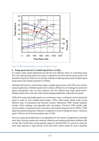
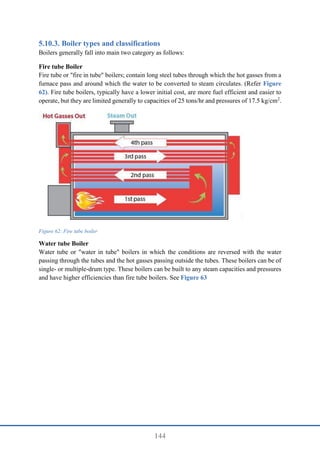
167. 153
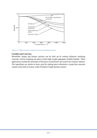
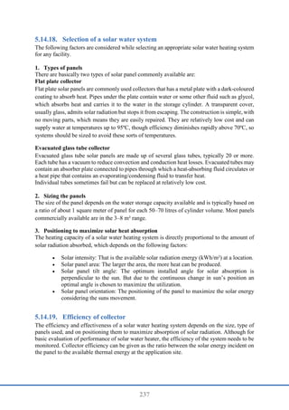
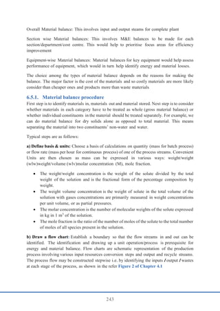
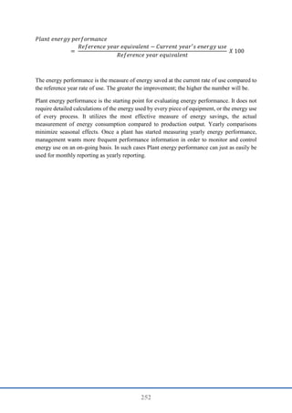
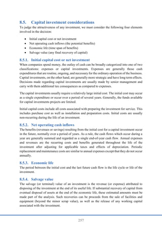
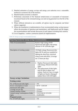
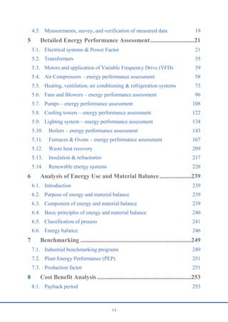
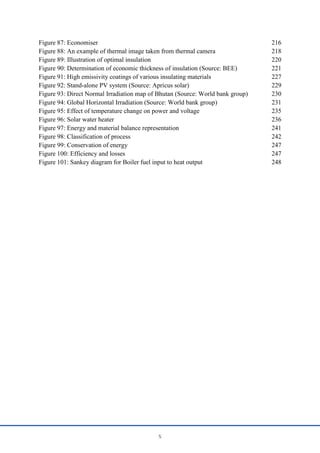
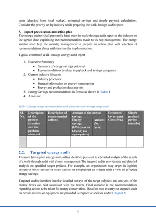
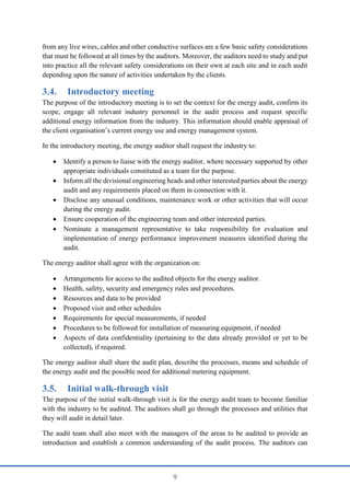
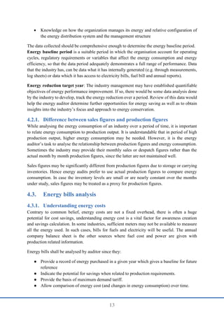
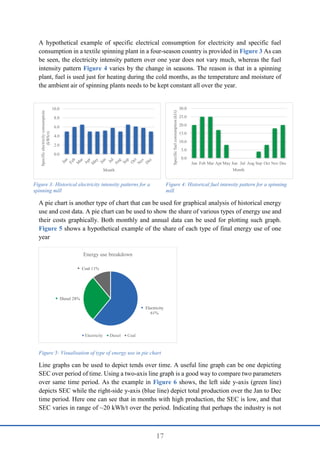
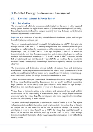
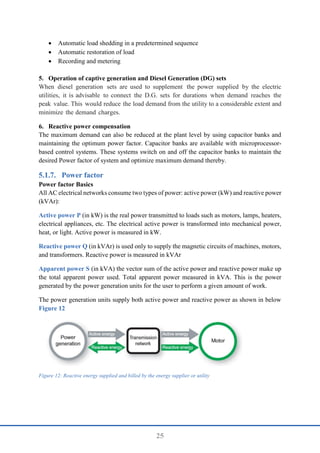
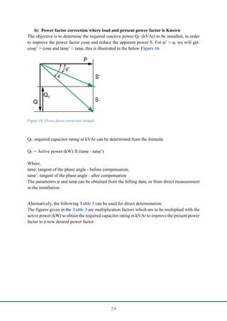
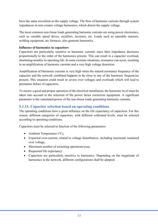
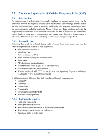
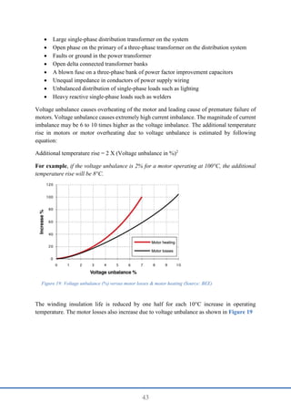
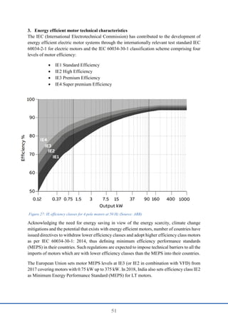
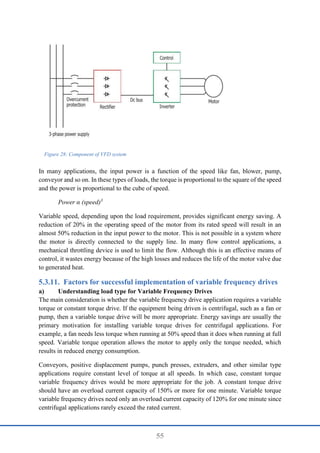
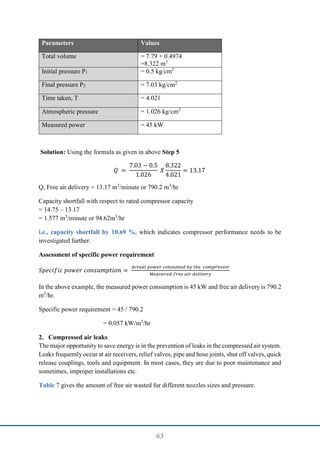
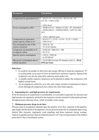
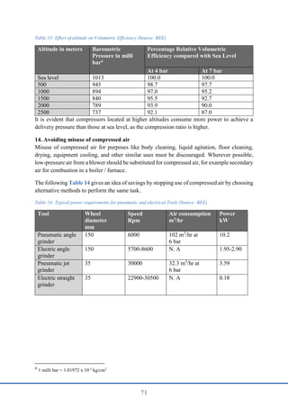
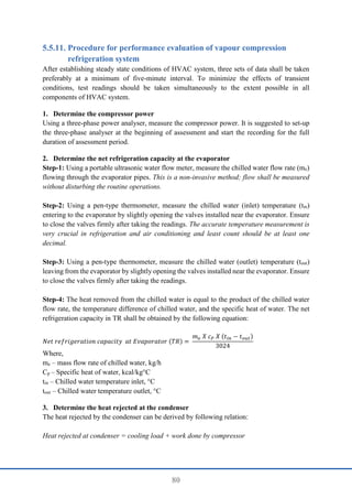
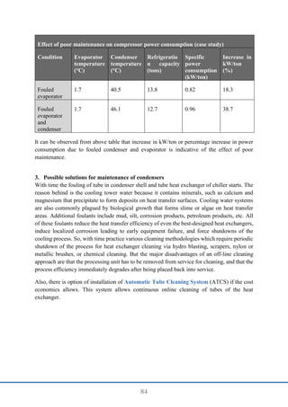
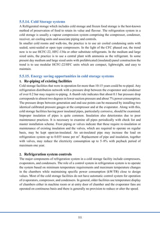
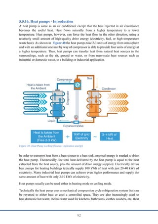
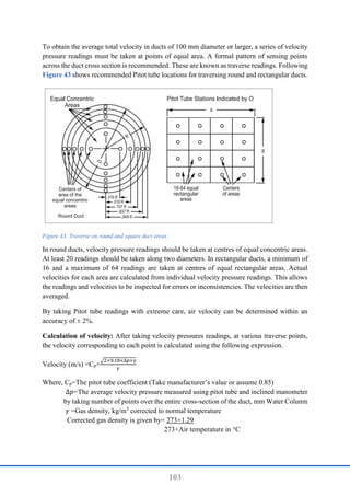
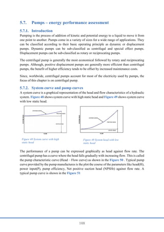
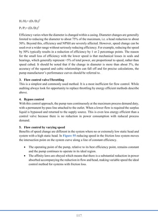
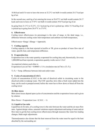
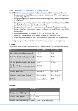
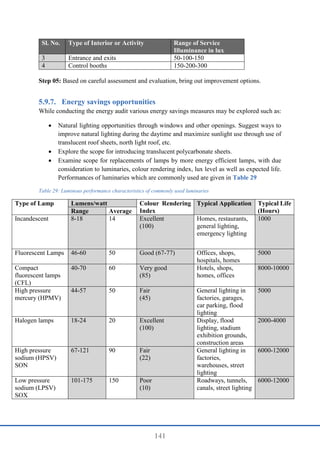
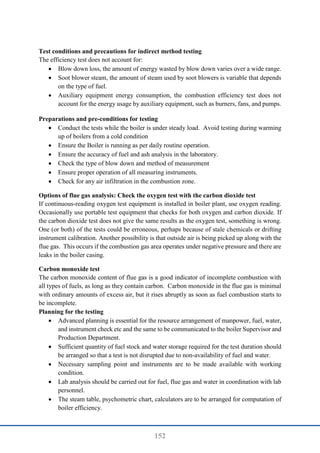
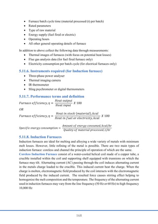
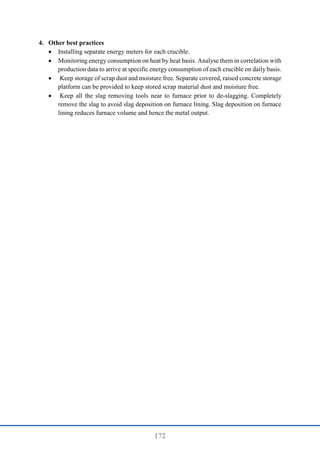
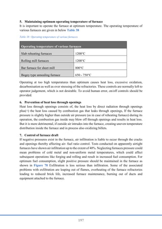
Boiler efficiency by indirect method: Calculation procedure and formula
In order to calculate the boiler efficiency by indirect method, all the losses that occur in the
boiler must be established. These losses are conveniently related to the amount of fuel burnt.
In this way it is easy to compare the performance of various boilers with different ratings.
However, it is suggested to get an ultimate analysis of the fuel periodically from a reputed
laboratory.
Theoretical (stoichiometric) air fuel ratio and excess air supplied are to be determined first for
computing the boiler losses. The formula is given below for the same.
Formulae for computing theoretical air fuel ratio and excess air supplied for combustion
Theoretical air required for
combustion
[(11.6 X C) + {34.8 X (H2 – O2/8)} + (4.35 X S)] / 100
kg/kg of fuel
from fuel analysis: Where C, H2, O2, and S are the
percentage of carbon, hydrogen, oxygen and sulphur
present in the fuel.
% Excess air supplied (EA)
=
O2%
21 − O2%
X 100
O2% to be obtained from flue gas analysis
Usually, O2 measurement is recommended, if O2
measurement is not available, use CO2 measurement and
below formula to obtain excess air
=
7900 X [(CO2%)t−(CO2%)a]
(CO2%)a X [100− (CO2%)t]
(CO2%)t is theoretical CO2
(CO2%)a is actual CO2% measured in flue gas
(CO2) t
=
Moles of C
(Moles 𝑁2 + Moles of C + Moles of S)
Moles of N2
=
(Weight of 𝑁2 in theoretical air)
(Molecular Weight of 𝑁2)
+
Weight of 𝑁2 in fuel
𝑀𝑜𝑙𝑒𝑐𝑢𝑙𝑎𝑟 𝑤𝑒𝑖𝑔ℎ𝑡 𝑜𝑓 𝑁2
Moles of C
=
𝑊𝑒𝑖𝑔ℎ𝑡 𝑜𝑓 𝐶 𝑖𝑛 𝑓𝑢𝑒𝑙
𝑀𝑜𝑙𝑒𝑐𝑢𝑙𝑎𝑟 𝑤𝑒𝑖𝑔ℎ𝑡 𝑜𝑓 𝐶
Moles of S
=
𝑊𝑒𝑖𝑔ℎ𝑡 𝑜𝑓 𝑆 𝑖𝑛 𝑓𝑢𝑒𝑙
𝑀𝑜𝑙𝑒𝑐𝑢𝑙𝑎𝑟 𝑤𝑒𝑖𝑔ℎ𝑡 𝑜𝑓 𝑆

168. 154
Formulae for computing theoretical air fuel ratio and excess air supplied for combustion
Actual mass or air supplied/kg
of fuel, AAS = (1 +
𝐸𝐴
100
) 𝑋 𝑡ℎ𝑒𝑜𝑟𝑒𝑡𝑖𝑐𝑎𝑙 𝑎𝑖𝑟
The various losses associated with the operation of a boiler are discussed below with required
formula
Various losses associated with operation of Boiler
Heat loss due to
dry flue gas in %
(L1)
=
𝑚 𝑋 𝐶𝑃𝑋 (𝑡𝑓 − 𝑡𝑎)
𝐺𝐶𝑉 𝑜𝑓 𝑓𝑢𝑒𝑙
𝑋 100
Where,
total mass of dry flue gas in (m)/kg of fuel = mass of CO2 in flue gas + mass of
SO2 in flue gas + mass of N2 content in fuel + mass of N2 in the combustion air
supplied + mass of O2 in flue gas
OR
Total mass of dry flue gas (m)/kg of fuel = Mass of actual air supplied (AAS) +
Mass of fuel supplied
Cp=Specific heat of flue gas in kcal/kg°C
tf= Temperature of flue gas in °C
ta= Temperature of ambient air in °C
Heat loss due to
formation of
water from H2 in
fuel in % (L2)
=
9 𝑋 𝐻2 𝑋 (584 + 𝐶𝑃 (𝑇𝑓 − 𝑇𝑎)
𝐺𝐶𝑉 𝑜𝑓 𝑓𝑢𝑒𝑙
𝑋 100
H2 = Kg of Hydrogen present in 1 kg fuel
Cp = Specific heat of superheated steam in kcal/kg°C
Tf = Flue gas temperature in °C
Ta = Ambient temperature in °C
584 = latent heat corresponding to the partial pressure of water vapour in kcal/kg
“The combustion of hydrogen causes a heat loss because the product of
combustion is water. This water is converted to steam and this carries away heat
in the form of its latent heat”.
Heat loss due to
moisture present
in fuel in % (L3)
=
𝑀 𝑋 (584 + 𝐶𝑃𝑋 (𝑡𝑓 − 𝑡𝑎)
𝐺𝐶𝑉 𝑜𝑓 𝑓𝑢𝑒𝑙
𝑋 100
M= Kg of moisture in 1 kg of fuel
Cp=Specific heat of superheated steam in kcal/kg°C
584= latent heat corresponding to the partial pressure of water vapour in kcal/kg
“Moisture entering the boiler with the fuel leaves as a superheated vapour”.

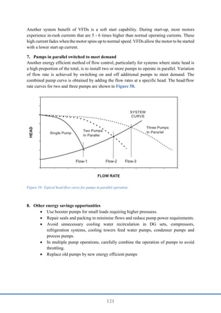
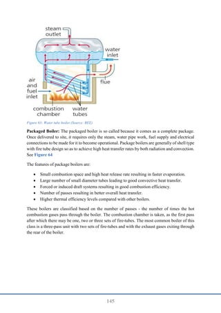
169. 155
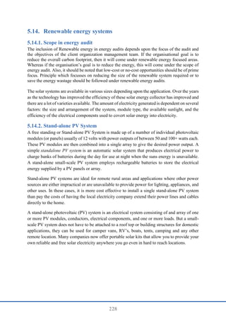
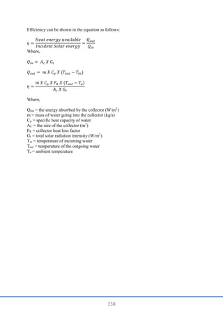
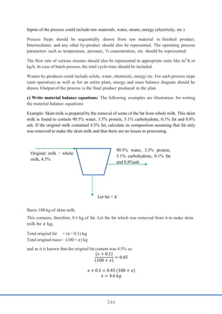
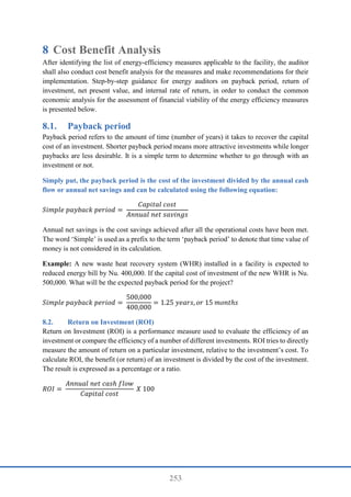
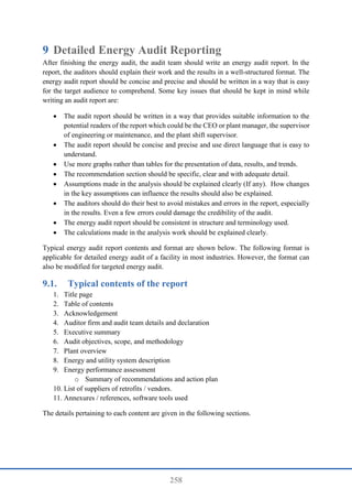
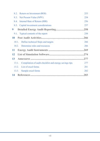
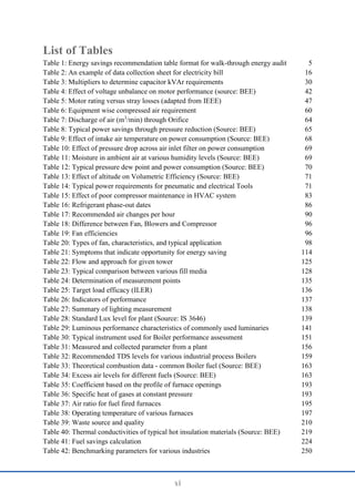
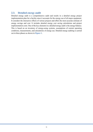
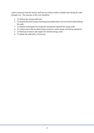
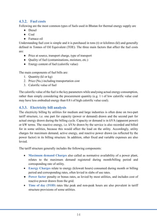
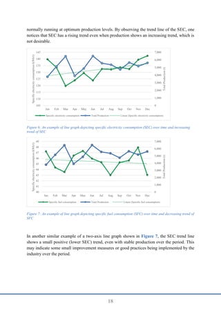
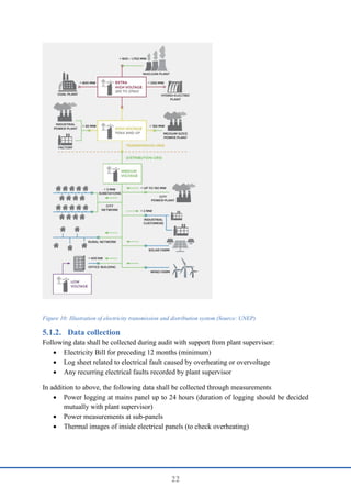
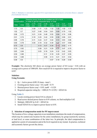
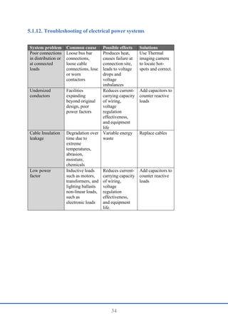
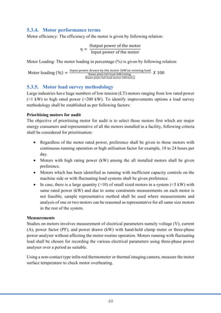
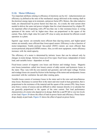
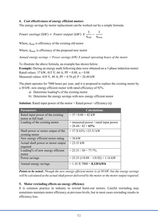
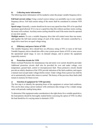
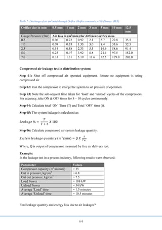
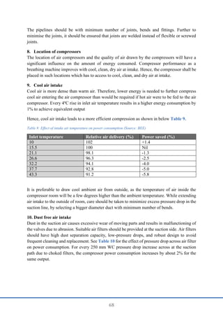
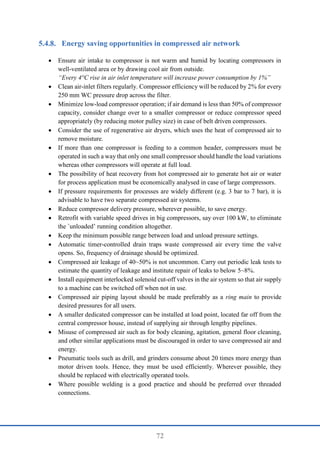
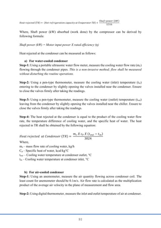
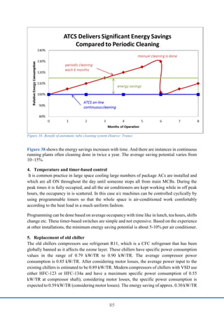
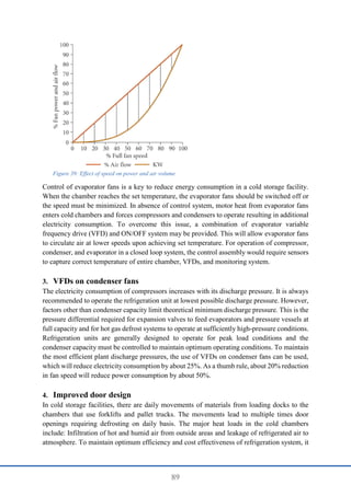
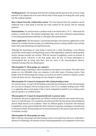
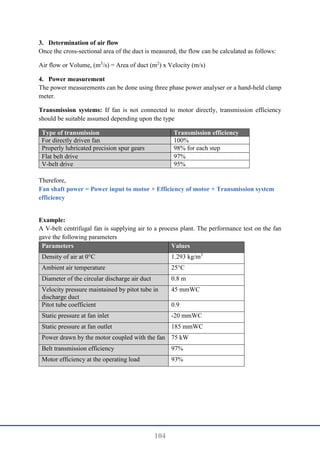
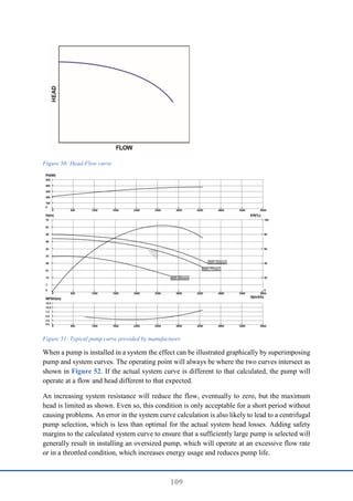
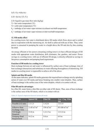
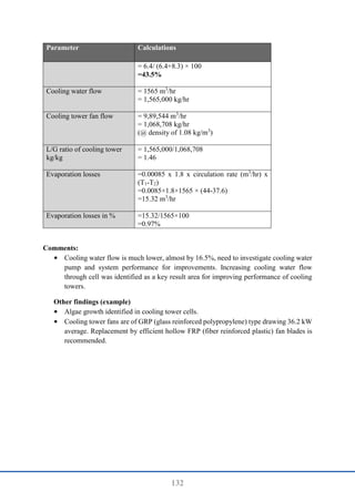
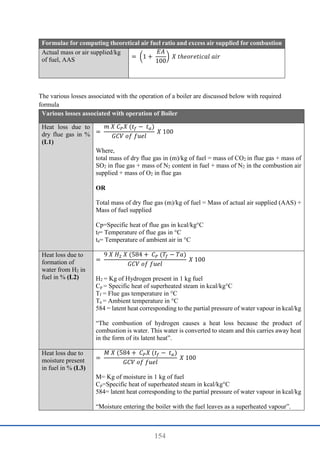
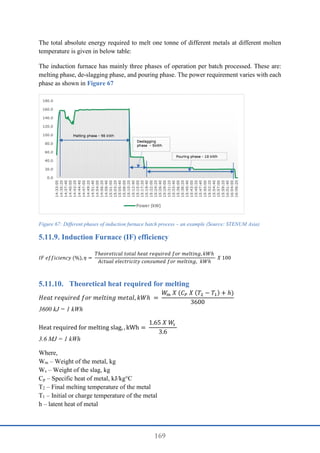
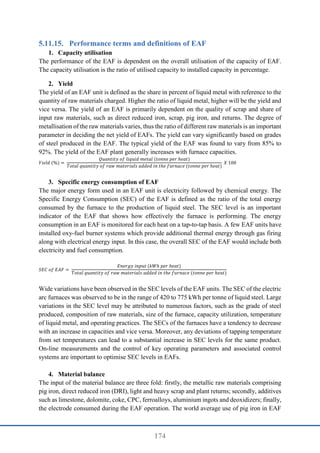
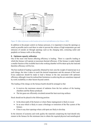
Various losses associated with operation of Boiler
Heat loss due to
moisture present
in air in % (L4)
=
𝐴𝐴𝑆 𝑋 ℎ𝑢𝑚𝑖𝑑𝑖𝑡𝑦 𝑋 𝐶𝑃𝑋 (𝑡𝑓 − 𝑡𝑎)
𝐺𝐶𝑉 𝑜𝑓 𝑓𝑢𝑒𝑙
𝑋 100
AAS = Actual mass of air supplied per kg of fuel
Humidity factor = kg of water/kg of dry air
Cp = Specific heat of superheat steam in kcal/kg°C
tf = flue gas temperature in °C
ta =ambient temperature in °C (dry bulb)
“Vapour in the form of humidity in the incoming air, is superheated as it passes
through the boiler. Since this heat passes up the stack, it must be included as a
boiler loss”.
Heat loss due to
partial conversion
of C to CO or
incomplete
combustion in %
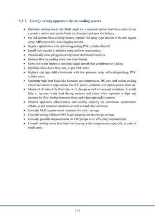
(L5)
=
%𝐶𝑂 𝑋 𝐶
%𝐶𝑂+% 𝐶𝑂2
𝑋
5654
𝐺𝐶𝑉 𝑜𝑓 𝑓𝑢𝑒𝑙
𝑋 100
CO = Volume of CO in flue gas (%)
(1% = 10,000 ppm)
CO2 = Actual volume of CO2 in flue gas
C = Carbon content kg/kg of fuel
“Carbon monoxide (CO) is the only gas whose concentration can be
determined conveniently in a boiler plant test”.
Heat loss due to
radiation and
convection in
W/m2
(L6)
= 0.548 × [(Ts / 55.55)4
- (Ta / 55.55)4
] + 1.957 X (Ts - Ta)1.25
X √[(1.968Vm +
68.9) /68.9]
Vm = wind velocity in m/s
Ts = Surface temperature
Ta = Ambient temperature
Normally surface loss and other unaccounted losses is assumed based on the
type and size of the boiler as given below
For industrial fire tube/packaged boiler = 1.5% to 2.5%
For industrial water tube boiler = 2 to 3%
For power station boiler = 0.4 to 1%
“The other heat losses from a boiler consist of the loss of heat by radiation and
convection from the boiler casting into the surrounding boiler house”.
Heat loss due to
unburnt in fly ash
in % (L7)
=
𝑇𝑜𝑡𝑎𝑙 𝑎𝑠ℎ 𝑐𝑜𝑒𝑐𝑡𝑒𝑑 𝑝𝑒𝑟 𝑘𝑔 𝑜𝑓 𝑓𝑢𝑒𝑙 𝑏𝑢𝑟𝑛𝑡 𝑋 𝐺𝐶𝑉 𝑜𝑓 𝑓𝑙𝑦 𝑎𝑠ℎ
𝐺𝐶𝑉 𝑜𝑓 𝑓𝑢𝑒𝑙
𝑋 100
Heat loss due to
unburnt in bottom
ash in % (L8)
=
𝑇𝑜𝑡𝑎𝑙 𝑎𝑠ℎ 𝑐𝑜𝑙𝑙𝑒𝑐𝑡𝑒𝑑 𝑝𝑒𝑟 𝑘𝑔 𝑜𝑓 𝑓𝑢𝑒𝑙 𝑏𝑢𝑟𝑛𝑡 𝑋 𝐺𝐶𝑉 𝑜𝑓 𝑏𝑜𝑡𝑡𝑜𝑚 𝑎𝑠ℎ
𝐺𝐶𝑉 𝑜𝑓 𝑓𝑢𝑒𝑙
𝑋 100
Example:

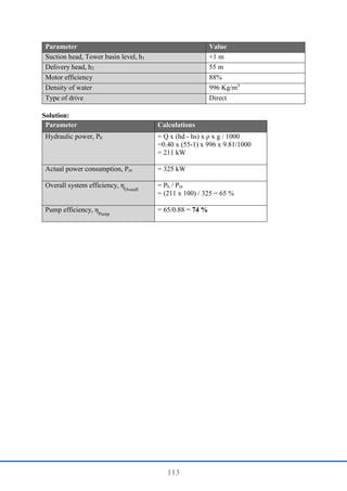
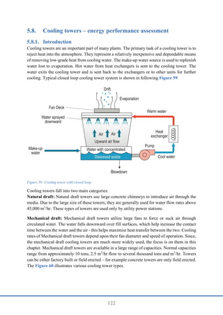
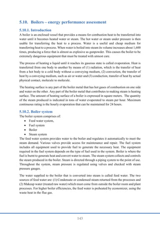
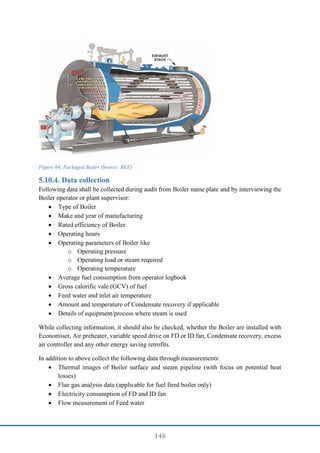
170. 156
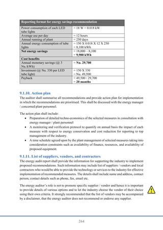
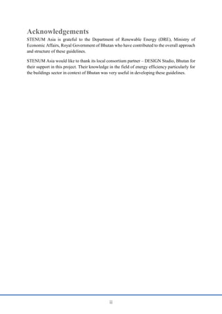
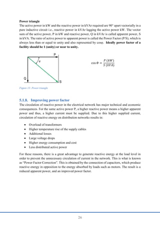
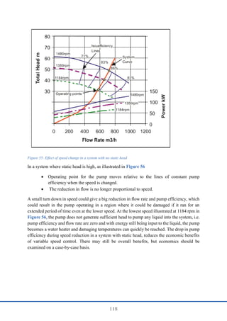
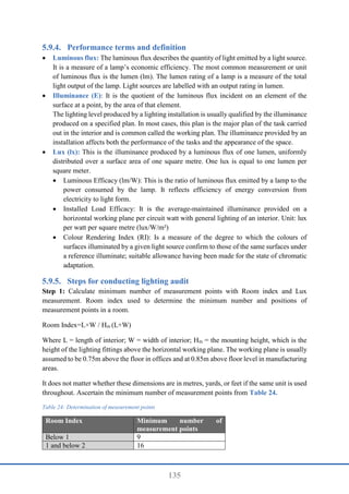
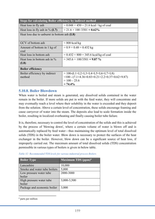
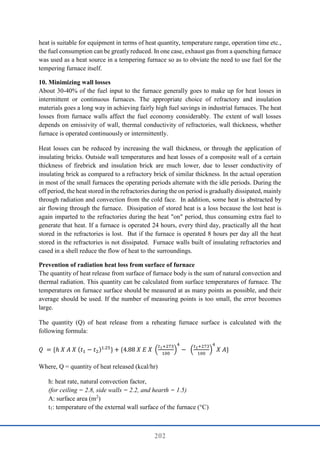
The following are the data collected for a boiler using coal as the fuel. Find out the boiler
efficiency by indirect method.
Table 31: Measured and collected parameter from a plant
Parameter Values
Fuel firing rate 5600 kg/hr
Steam generation rate 21940 kg/hr
Steam pressure 43 kg/cm2
Steam temperature 377°C
Feed water temperature 96°C
%O2 in flue gas 2.75%
Average flue gas temperature 190°C
Ambient temperature 31°C
Humidity in ambient air 0.0204 kg/kg dry air
Surface temperature of boiler 70°C
Wind velocity around boiler 3.5 m/s
Total surface area of boiler 90 m2
GCV of bottom ash 800 kcal/kg
GCV of fly ash 450 kcal/kg
Ratio of bottom ash to fly ash 90:10
Fuel analysis in %
Ash 48%
Moisture 4.4%
Carbon 36%
Hydrogen 2.6%
Nitrogen 1.1%
Oxygen 7.3%
Sulphur 0.6
GCV 3501 kcal/kg
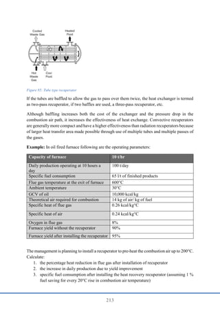
Solution: Boiler efficiency by indirect method
Steps for calculating Boiler efficiency by indirect method
Step-1 Find theoretical air requirement for complete combustion
Theoretical air required for
combustion
[(11.6 X C) + {34.8 X (H2 – O2/8)} + (4.35 X S)] / 100
kg/kg of fuel
= [(11.6 X 36) + {34.8 X (2.6 – 7.3/8)} + (4.35 X 0.6)] /
100
= 4.79 kg/kg of coal
Step-2 Find CO2% at theoretical condition, (CO2) t
(CO2) t =Moles of C/ (Moles N2+Moles of C+ Moles of S)
Moles of N2 = (Weight of N2 in theoretical air/ Mol. Weight of N2) +
(Weight of N2 in fuel / Mol Weight of N2)
= (4.79× (77/100)/28) +(0.011/28)
=0.1321
Moles of C = 0.36/12= 0.03

171. 157
Steps for calculating Boiler efficiency by indirect method
Moles of S = 0.006/32= 0.0001875
(CO2) t = 0.03/ (0.03+0.1321+0.0001875)
= 18.48 %
Step 3- To find Excess air supplied
Actual O2 measured in flue gas =2.75%
% Excess air supplied (EA)
=
𝑂2%
21 − 𝑂2%
𝑋 100
=
2.75%
21−2.75%
𝑋 100 = 15%
Step 4- To find actual mass of air supplied, AAS
AAS
= (1 +
𝐸𝐴
100
) 𝑋 𝑡ℎ𝑒𝑜𝑟𝑒𝑡𝑖𝑐𝑎𝑙 𝑎𝑖𝑟
= (1 +
15
100
) 𝑋 4.79
= 5.51 kg/kg of coal
Step 5- To find actual mass of dry flue gas
Actual mass of dry flue gas = Mass of actual air supplied + Mass of fuel supplied
= 5.51+1
=6.51 kg/kg of coal
Step 6- To find all the losses
Heat loss in dry flue gas (L1)
=
𝑚 𝑋 𝐶𝑃𝑋 (𝑡𝑓 − 𝑡𝑎)
𝐺𝐶𝑉 𝑜𝑓 𝑓𝑢𝑒𝑙
𝑋 100
=
6.51 𝑋 0.24 𝑋 (190 − 31)
3501
𝑋 100
= 7.1%
Cp =Specific heat of flue gas = 0.24 kcal/kg°C
% Heat loss due to formation of
water from H2 in fuel (L2) =
9 𝑋 𝐻2 𝑋 (584 + 𝐶𝑃 (𝑇𝑓 − 𝑇𝑎)
𝐺𝐶𝑉 𝑜𝑓 𝑓𝑢𝑒𝑙
𝑋 100
=
9 𝑋 0.026 𝑋 (584 + 0.45 (190 − 31)
3501
𝑋 100
= 4.36%
Cp = Specific heat of superheated steam
=0.45 kcal/kg°C

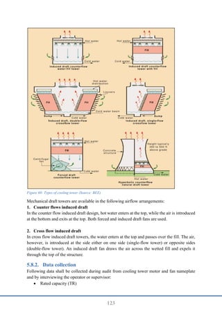
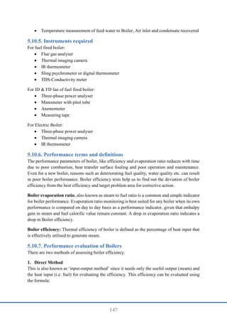
172. 158
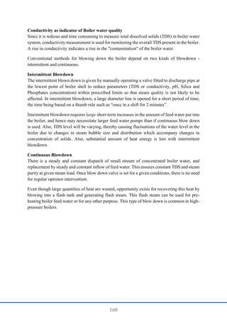
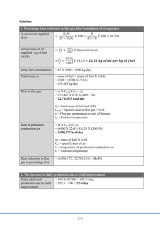
Steps for calculating Boiler efficiency by indirect method
Heat loss due to moisture in fuel
(L3) =
𝑀 𝑋 (584 + 𝐶𝑃𝑋 (𝑡𝑓 − 𝑡𝑎)
𝐺𝐶𝑉 𝑜𝑓 𝑓𝑢𝑒𝑙
𝑋 100
=
0.044 𝑋 (584 + 0.43 𝑋 (190 − 31)
3501
𝑋 100
= 0.83%
Heat loss due to moisture in air
(L4) =
𝐴𝐴𝑆 𝑋 ℎ𝑢𝑚𝑖𝑑𝑖𝑡𝑦 𝑋 𝐶𝑃𝑋 (𝑡𝑓 − 𝑡𝑎)
𝐺𝐶𝑉 𝑜𝑓 𝑓𝑢𝑒𝑙
𝑋 100
=
5.51 𝑋 0.0204 𝑋 0.43 (190− 31)
3501
𝑋 100
= 0.21%
Heat loss due to partial
conversion of C to CO (L5)
=
%𝐶𝑂 𝑋 𝐶
%𝐶𝑂+% 𝐶𝑂2
𝑋
5654
𝐺𝐶𝑉 𝑜𝑓 𝑓𝑢𝑒𝑙
𝑋 100
=
0.55 𝑋 0.36
0.55 +14
𝑋
5654
3501
𝑋 100
= 2.2%
Heat loss due to radiation and
convection in W/m2
(L6)
= 0.548 × [(Ts / 55.55)4 - (Ta / 55.55)4] + 1.957 X (Ts -
Ta)1.25 X √[(1.968Vm + 68.9) /68.9]
= 0.548 × [(343/55.55)4
-(304/55.55)4
] + 1.957 X (343-
304)1.25
X √[(196.85 X 3.5 + 68.9)/68.9)
= 937.62 W/m2
(1 W = 0.86 kcal)
= 937.67×0.86 = 806.35 kcal/m2
Total radiation and convection
loss per hour
= Heat loss due to radiation and convection X total surface
area of boiler
= 806.35 X 90 = 72,571.6 kcal/hr
Heat loss due radiation and
convection loss in % (L6)
= (total radiation and convection loss per hour) / (GCV of
fuel X Fuel firing rate)
= (72,571.6) / (3501 X 5600)
= 0.0037
= 0.0037 X 100 = 0.37%
Heat loss due to unburnt in fly ash (L7)
% ash in coal = 48
Ratio of bottom ash to fly ash = 90:10
GCV of fly ash = 450 kcal/kg
Amount of fly ash in 1 kg of
coal
= 0.1 × 0.48 = 0.048 kg

173. 159
Steps for calculating Boiler efficiency by indirect method
Heat loss in fly ash = 0.048 × 450 = 21.6 kcal / kg of coal
Heat loss in fly ash in % (L7) = 21.6 × 100 /3501 = 0.62%
Heat loss due to unburnt in bottom ash (L8)
GCV of bottom ash = 800 kcal/kg
Amount of bottom in 1 kg of
coal
= 0.9 × 0.48 = 0.432 kg
Heat loss in bottom ash = 0.432 × 800 = 345.6 kcal/kg of coal
Heat loss in bottom ash in %
(L8)
= 345.6 × 100/3501 = 9.87 %
Boiler efficiency
Boiler efficiency by indirect
method
= 100-(L1+L2+L3+L4+L5+L6+L7+L8)
=100 - (7.1+4.36+0.83+0.21+2.2+0.37+0.62+9.87)
= 100 – 25.6
= 74.4%
Boiler Blowdown
When water is boiled and steam is generated, any dissolved solids contained in the water
remain in the boiler. If more solids are put in with the feed water, they will concentrate and
may eventually reach a level where their solubility in the water is exceeded and they deposit
from the solution. Above a certain level of concentration, these solids encourage foaming and
cause carryover of water into the steam. The deposits also lead to scale formation inside the
boiler, resulting in localized overheating and finally causing boiler tube failure.
It is, therefore, necessary to control the level of concentration of the solids and this is achieved
by the process of 'blowing down', where a certain volume of water is blown off and is
automatically replaced by feed water - thus maintaining the optimum level of total dissolved
solids (TDS) in the boiler water. Blow down is necessary to protect the surfaces of the heat
exchanger in the boiler. However, blow down can be a significant source of heat loss, if
improperly carried out. The maximum amount of total dissolved solids (TDS) concentration
permissible in various types of boilers is given in below table.
Table 32: Recommended TDS levels for various industrial process Boilers
Boiler Type Maximum TDS (ppm)6
Lancashire 10,000
Smoke and water tube boilers 5,000
Low pressure water tube
boiler
2000-3000
High pressure water tube
boiler
3,000-3,500
Package and economic boiler 3,000
6
parts per million

174. 160
Conductivity as indicator of Boiler water quality
Since it is tedious and time consuming to measure total dissolved solids (TDS) in boiler water
system, conductivity measurement is used for monitoring the overall TDS present in the boiler.
A rise in conductivity indicates a rise in the "contamination" of the boiler water.
Conventional methods for blowing down the boiler depend on two kinds of blowdown -
intermittent and continuous.
Intermittent Blowdown
The intermittent blown down is given by manually operating a valve fitted to discharge pipe at
the lowest point of boiler shell to reduce parameters (TDS or conductivity, pH, Silica and
Phosphates concentration) within prescribed limits so that steam quality is not likely to be
affected. In intermittent blowdown, a large diameter line is opened for a short period of time,
the time being based on a thumb rule such as “once in a shift for 2 minutes”.
Intermittent blowdown requires large short-term increases in the amount of feed water put into
the boiler, and hence may necessitate larger feed water pumps than if continuous blow down
is used. Also, TDS level will be varying, thereby causing fluctuations of the water level in the
boiler due to changes in steam bubble size and distribution which accompany changes in
concentration of solids. Also, substantial amount of heat energy is lost with intermittent
blowdown.
Continuous Blowdown
There is a steady and constant dispatch of small stream of concentrated boiler water, and
replacement by steady and constant inflow of feed water. This ensures constant TDS and steam
purity at given steam load. Once blow down valve is set for a given conditions, there is no need
for regular operator intervention.
Even though large quantities of heat are wasted, opportunity exists for recovering this heat by
blowing into a flash tank and generating flash steam. This flash steam can be used for pre-
heating boiler feed water or for any other purpose. This type of blow down is common in high-
pressure boilers.

175. 161
Figure 66: Blowdown heat recovery system
Blowdown calculations
The quantity of blowdown required to control boiler water solids concentration is calculated
by using the following formula:
Blow down (%) =
Feed water TDS X Make up water %
Maximum permissible TDS in Boiler water − Feed water TDS
X 100
If maximum permissible limit of TDS as in a package boiler is 3000 ppm, percentage make up
water is 10% and TDS in feed water is 300 ppm, then the percentage blow down is given as:
Blow down (%) =
300 X 10%
3000 − 300
X 100 = 1.11%
If boiler evaporation rate is 3000 kg/hr then required blow down rate is:
3000 X 1.11 % = 33.3 kg/hr
Benefits of Blowdown
Good boiler blow down control can significantly reduce treatment and operational costs that
include:
 Lower pre-treatment costs
 Less make-up water consumption
 Reduced maintenance downtime
 Increased boiler life
 Lower consumption of treatment chemicals

176. 162
Energy savings opportunities in Boiler
The various energy efficiency opportunities in boiler system can be related to combustion, heat
transfer, avoidable losses, high auxiliary power consumption, water quality and blowdown.
Examining the following factors can indicate if a boiler is being run to maximize its efficiency:
1. Stack temperature
The stack temperature should be as low as possible. However, it should not be so low that water
vapour in the exhaust condenses on the stack walls. This is important in fuels containing
significant sulphur as low temperature can lead to sulphur dew point corrosion. Stack
temperatures greater than 200°C indicates potential for recovery of waste heat. It also indicates
the scaling of heat transfer/recovery equipment and hence the urgency of taking an early shut
down for water / flue side cleaning.
2. Feed water preheating using economiser
Typically, the flue gases leaving a modern 3-pass shell boiler are at temperatures of 200 to
300°C. Thus, there is a potential to recover heat from these gases. The flue gas exit temperature
from a boiler is usually maintained at a minimum of 200°C, so that the sulphur oxides in the
flue gas do not condense and cause corrosion in heat transfer surfaces. When a clean fuel such
as natural gas, LPG or gas oil is used, the economy of heat recovery must be worked out, as
the flue gas temperature may be well below 200°C.
The potential for energy saving depends on the type of boiler installed and the fuel used. For a
typically older model shell boiler, with a flue gas exit temperature of 260°C, an economizer
could be used to reduce it to 200°C, increasing the feed water temperature by 15°C. Increase
in overall thermal efficiency would be in the order of 3%. For a modern 3-pass shell boiler
firing natural gas with a flue gas exit temperature of 140°C. A condensing economizer would
reduce the exit temperature to 65°C increasing thermal efficiency by 5%.
3. Combustion air preheat
Combustion air preheating is an alternative to feedwater heating. In order to improve thermal
efficiency by 1%, the combustion air temperature must be raised by 20°C. Most gas and oil
burners used in a boiler plant are not designed for high air preheat temperatures.
Modern burners can withstand much higher combustion air preheat, so it is possible to consider
such units as heat exchangers in the exit flue as an alternative to an economizer, when either
space or a high feed water return temperature make it viable.
4. Incomplete combustion
Incomplete combustion can arise from a shortage of air or surplus of fuel or poor distribution
of fuel. It is usually obvious from the colour or smoke and must be corrected immediately.
In the case of oil and gas fired systems, CO, or smoke (for oil fired systems only) with normal
or high excess air indicates burner system problems. A more frequent cause of incomplete
combustion is the poor mixing of fuel and air at the burner. Poor oil fires can result from

177. 163
improper viscosity, worn tips, carbonization on tips and deterioration of diffusers or spinner
plates.
With coal firing, unburned carbon can comprise a big loss. It occurs as grit carry-over or
carbon-in-ash and may amount to more than 2% of the heat supplied to the boiler. Non uniform
fuel size could be one of the reasons for incomplete combustion. In chain grate stokers, large
lumps will not burn out completely, while small pieces and fines may block the air passage,
thus causing poor air distribution. In sprinkler stokers, stoker grate condition, fuel distributors,
wind box air regulation and over-fire systems can affect carbon loss. Increase in the fines in
pulverized coal also increases carbon loss.
5. Excess air control
The Table 33 gives the theoretical amount of air required for combustion of various types of
fuel. Excess air is required in all practical cases to ensure complete combustion, to allow for
the normal variations in combustion and to ensure satisfactory stack conditions for some fuels.
Table 33: Theoretical combustion data - common Boiler fuel (Source: BEE)
Fuel kg of air
required/kg
of fuel
kg of
flue
gas/kg
of fuel
m3 of
flue/kg
of fuel
Theoretical
CO2 % in
dry flue gas
CO2 % in
flue
gas
achieved
in
practice
Bagasse 3.2 3.43 2.61 20.65 10-12
Coal
(bituminous)
10.8 11.7 9.40 18.70 10-13
Lignite 8.4 9.10 6.97 19.40 9-13
Paddy Husk 4.6 5.63 4.58 19.8 14-15
Wood 5.8 6.4 4.79 20.3 11.13
Furnace Oil 13.90 14.30 11.50 15.0 9-14
LSHS 14.04 14.63 10.79 15.5 9-14
The optimum excess air level for maximum boiler efficiency occurs when the sum of the losses
due to incomplete combustion and loss due to heat in flue gases is minimum. This level varies
with furnace design, type of burner, fuel and process variables. It can be determined by
conducting tests with different air fuel ratios. Typical values of excess air supplied for various
fuels are given in Table 34
Table 34: Excess air levels for different fuels (Source: BEE)
Fuel Type of Furnace or Burners Excess Air
(% by
weight)
Pulverized
coal
Completely water-cooled furnace for slag tap or dry ash
removal
15-20
Partially water-cooled furnace for dry-ash removal 15-40

178. 164
Fuel Type of Furnace or Burners Excess Air
(% by
weight)
Coal Spreader stoker 30-60
Water-cooler vibrating-grate stokers 30-60
Chain-grate and traveling-gate stokers 15-50
Underfeed stoker 20-50
Fuel oil Oil burners register type 15-20
Multi-fuel burners and flat flame 20-30
Natural
gas
High pressure burner 5-7
Wood Dutch over (10-23%through grates) and Hofft type 20-25
Bagasse All furnaces 25-35
Black
liquor
Recovery furnaces for draft and soda-pulping processes 30-40
Controlling excess air to an optimum level always results in reduction in flue gas losses; for
every 1% reduction in excess air there is approximately 0.6% rise in efficiency.
Various methods are available to control the excess air:
 Portable oxygen analysers and draft gauges can be used to make periodic readings to
guide the operator to manually adjust the flow of air for optimum operation. Excess air
reduction up to 20% is feasible.
 The most common method is the continuous oxygen analyser with a local readout
mounted draft gauge, by which the operator can adjust air flow. A further reduction of
10-15% can be achieved over the previous system.
 The same continuous oxygen analyser can have a remote controlled pneumatic damper
positioner, by which the readouts are available in a control room. This enables an
operator to remotely control a number of firing systems simultaneously.
 The most sophisticated system is the automatic stack damper control, whose cost is
really justified only for large systems.
6. Radiation and convection heat Loss
The external surfaces of a shell boiler are hotter than the surroundings. The surfaces thus lose
heat to the surroundings depending on the surface area and the difference in temperature
between the surface and the surroundings.
The heat loss from the boiler shell is normally a fixed energy loss, irrespective of the boiler
output. With modern boiler designs, this may represent only 1.5% on the gross calorific value
at full rating, but will increase to around 6%, if the boiler operates at only 25 percent output.
Repairing or augmenting insulation can reduce heat loss through boiler walls and piping.
7. Automatic blowdown control
Uncontrolled continuous blowdown is very wasteful. Automatic blowdown controls can be
installed that sense and respond to boiler water conductivity and pH. A 10% blow down
operating at 15 kg/cm2
pressure in a boiler will result in 3% efficiency loss.

179. 165
8. Reduction of scaling and soot losses
In oil and coal-fired boilers, soot build-up on tubes acts as an insulator against heat transfer.
Any such deposits should be removed on a regular basis. Elevated stack temperatures may
indicate excessive soot build-up. Also, same result will occur due to scaling on the water side.
High exit gas temperatures at normal excess air indicate poor heat transfer performance. This
condition can result from a gradual build-up of gas-side or waterside deposits. Waterside
deposits require a review of water treatment procedures and tube cleaning to remove deposits.
An estimated 1% efficiency loss occurs with every 22°C increase in stack temperature.
Stack temperature should be checked and recorded regularly as an indicator of soot deposits.
When the flue gas temperature rises about 20°C above the temperature for a newly cleaned
boiler, it is time to remove the soot deposits. It is, therefore, recommended to install a dial type
thermometer at the base of the stack to monitor the exhaust flue gas temperature.
It is estimated that 3 mm of soot can cause an increase in fuel consumption by 2.5% due to
increased flue gas temperatures. Periodic off-line cleaning of radiant furnace surfaces, boiler
tube banks, economizers and air heaters may be necessary to remove stubborn deposits.
9. Reduction of Boiler steam pressure
This is an effective means of reducing fuel consumption, if permissible, by as much as 1 to 2%.
Lower steam pressure gives a lower saturated steam temperature and without stack heat
recovery, a similar reduction in the temperature of the flue gas temperature results.
Steam is generated at pressures normally dictated by the highest pressure / temperature
requirements for a particular process. In some cases, the process does not operate all the time,
and there are periods when the boiler pressure could be reduced. The energy manager should
consider pressure reduction carefully, before recommending it. Adverse effects, such as an
increase in water carryover from the boiler owing to pressure reduction, may negate any
potential saving. Pressure should be reduced in stages, and no more than a 20 percent reduction
should be considered.
10. Variable speed control for Fans, Blowers and Pumps
Variable speed control is an important means of achieving energy savings. Generally,
combustion air control is affected by throttling dampers fitted at forced and induced draft fans.
Though dampers are simple means of control, they lack accuracy, giving poor control
characteristics at the top and bottom of the operating range. In general, if the load characteristic
of the boiler is variable, the possibility of replacing the dampers by a VSD should be evaluated.
11. Effect of Boiler loading on efficiency
The maximum efficiency of the boiler does not occur at full load, but at about two-thirds of the
full load. If the load on the boiler decreases further, efficiency also tends to decrease. At zero
output, the efficiency of the boiler is zero, and any fuel fired is used only to supply the losses.
The factors affecting boiler efficiency are:
 As the load falls, so does the value of the mass flow rate of the flue gases through the
tubes. This reduction in flow rate for the same heat transfer area, reduced the exit flue
gas temperatures by a small extent, reducing the sensible heat loss.

180. 166
 Below half load, most combustion appliances need more excess air to burn the fuel
completely. This increases the sensible heat loss.
In general, efficiency of the boiler reduces significantly below 25% of the rated load and as far
as possible, operation of boilers below this level should be avoided.
12. Proper Boiler scheduling
Since, the optimum efficiency of boilers occurs at 65-85% of full load, it is usually more
efficient, overall, to operate a fewer number of boilers at higher loads, than to operate a large
number at low loads.
13. Boiler replacement
The potential savings from replacing a boiler depend on the anticipated change in overall
efficiency. A change in a boiler can be financially attractive if the existing boiler is:
 old and inefficient
 not capable of firing cheaper substitution fuel
 over or under-sized for present requirements
 not designed for ideal loading conditions
The feasibility study should examine all implications of long-term fuel availability and
company growth plans. All financial and engineering factors should be considered. Since boiler
plants traditionally have a useful life of well over 25 years, replacement must be carefully
studied.

181. 167
5.11. Furnaces & Ovens – energy performance assessment
Furnace
A furnace is an equipment to melt metals for casting or heat materials for change of shape
(rolling, forging, etc.) or for change of properties (heat treatment).
Type and classification of difference furnaces
Based on the method of generating heat, furnaces are broadly classified into two types namely
combustion type (using fuels) and electric type. The combustion type furnace can be broadly
classified as oil fired, coal fired, or gas fired, depending upon the kind of combustion.
 Based on the mode of charging of material furnaces can be classified as (a) Intermittent
or Batch type furnace or Periodical furnace and (b) Continuous furnace.
 Based on mode of waste heat recovery as recuperative and regenerative furnaces.
 Another type of furnace classification is made based on mode of heat transfer, mode of
charging and mode of heat recovery.
The electric furnaces can be broadly classified as resistance type for heating and induction arc
for melting of metals.
Characteristics of an efficient furnace
A furnace should be designed so that in a given time, as much of material as possible can be
heated to a uniform temperature as possible with the least possible fuel and labour. To achieve
this end, the following parameters can be considered.
 Determination of the quantity of heat to be imparted to the material or charge.
 Liberation of sufficient heat within the furnace to heat the stock and overcome all heat
losses.
 Transfer of available part of that heat from the furnace gases to the surface of the
heating stock.
 Equalisation of the temperature within the stock.
 Reduction of heat losses from the furnace to the minimum possible extent.
Furnace energy supply
Since the products of flue gases directly contact the stock, type of fuel chosen is of importance.
For example, some materials will not tolerate sulphur in the fuel. Also use of solid fuels will
generate particulate matter, which will interfere with the stock place inside the furnace. Hence,
vast majority of the furnaces use liquid fuel, gaseous fuel or electricity as energy input.
Electricity is used in induction and arc furnaces for melting steel and cast iron. Non-ferrous
melting utilizes oil as fuel.
Data collection (for any type of furnace)
Following data shall be collected through observation and by interviewing furnace operator or
supervisor:
 Furnace capacity

182. 168
 Furnace batch cycle time (material processed (t) per batch)
 Rated parameters
 Type of raw material
 Energy supply (fuel fired or electric)
 Operating hours
 All other general operating details of furnace
In addition to above collect the following data through measurements:
 Thermal images of furnaces (with focus on potential heat losses)
 Flue gas analysis data (for fuel fired furnace only)
 Electricity consumption per batch cycle (for electrical furnaces only)
Instruments required (for Induction furnace)
 Three-phase power analyser
 Thermal imaging camera
 IR thermometer
 Sling psychrometer or digital thermometers
Performance terms and definition
𝐹𝑢𝑟𝑛𝑎𝑐𝑒 𝑒𝑓𝑓𝑖𝑐𝑖𝑒𝑛𝑐𝑦, 𝜂 =
𝐻𝑒𝑎𝑡 𝑜𝑢𝑡𝑝𝑢𝑡
𝐻𝑒𝑎𝑡 𝑖𝑛𝑝𝑢𝑡
𝑋 100
OR
𝐹𝑢𝑟𝑛𝑎𝑐𝑒 𝑒𝑓𝑓𝑖𝑐𝑖𝑒𝑛𝑐𝑦, 𝜂 =
𝐻𝑒𝑎𝑡 𝑖𝑛 𝑠𝑡𝑜𝑐𝑘 (𝑚𝑎𝑡𝑒𝑟𝑖𝑎𝑙), 𝑘𝑐𝑎𝑙
𝐻𝑒𝑎𝑡 𝑖𝑛 𝑓𝑢𝑒𝑙 𝑜𝑟 𝑒𝑙𝑒𝑐𝑡𝑟𝑖𝑐𝑖𝑡𝑦, 𝑘𝑐𝑎𝑙
𝑋 100
𝑆𝑝𝑒𝑐𝑖𝑓𝑖𝑐 𝑒𝑛𝑒𝑟𝑔𝑦 𝑐𝑜𝑛𝑠𝑢𝑚𝑝𝑡𝑖𝑜𝑛 =
𝐴𝑚𝑜𝑢𝑛𝑡 𝑜𝑓 𝑒𝑛𝑒𝑟𝑔𝑦 𝑐𝑜𝑛𝑠𝑢𝑚𝑒𝑑, 𝑘𝑐𝑎𝑙/ℎ𝑟
𝑄𝑢𝑎𝑙𝑖𝑡𝑦 𝑜𝑓 𝑚𝑎𝑡𝑒𝑟𝑖𝑎𝑙 𝑝𝑟𝑜𝑐𝑒𝑠𝑠𝑒𝑑, 𝑡/ℎ𝑟
Induction Furnaces
Induction furnaces are ideal for melting and alloying a wide variety of metals with minimum
melt losses. However, little refining of the metal is possible. There are two main types of
induction furnace: coreless and channel the principle of operation of which are the same.
Coreless Induction Furnace consist of a water-cooled helical coil made of a copper tube, a
crucible installed within the coil and supporting shell equipped with trunnions on which the
furnace may tilt. Alternating current (AC) passing through the coil induces alternating current
in the metals charge loaded to the crucible. This induced current heat the charge. When the
charge is molten, electromagnetic field produced by the coil interacts with the electromagnetic
field produced by the induced current. The resulted force causes stirring effect helping to
homogenize the melt composition and the temperature. The frequency of the alternating current
used in induction furnaces may vary from the line frequency (50 Hz or 60 Hz) to high frequency
10,000 Hz

183. 169
The total absolute energy required to melt one tonne of different metals at different molten
temperature is given in below table:
The induction furnace has mainly three phases of operation per batch processed. These are:
melting phase, de-slagging phase, and pouring phase. The power requirement varies with each
phase as shown in Figure 67
Figure 67: Different phases of induction furnace batch process – an example (Source: STENUM Asia)
Induction Furnace (IF) efficiency
𝐼𝐹 𝑒𝑓𝑓𝑖𝑐𝑖𝑒𝑛𝑐𝑦 (%), 𝜂 =
𝑇ℎ𝑒𝑜𝑟𝑒𝑡𝑖𝑐𝑎𝑙 𝑡𝑜𝑡𝑎𝑙 ℎ𝑒𝑎𝑡 𝑟𝑒𝑞𝑢𝑖𝑟𝑒𝑑 𝑓𝑜𝑟 𝑚𝑒𝑙𝑡𝑖𝑛𝑔, 𝑘𝑊ℎ
𝐴𝑐𝑡𝑢𝑎𝑙 𝑒𝑙𝑒𝑐𝑡𝑟𝑖𝑐𝑖𝑡𝑦 𝑐𝑜𝑛𝑠𝑢𝑚𝑒𝑑 𝑓𝑜𝑟 𝑚𝑒𝑙𝑡𝑖𝑛𝑔, 𝑘𝑊ℎ
𝑋 100
Theoretical heat required for melting
𝐻𝑒𝑎𝑡 𝑟𝑒𝑞𝑢𝑖𝑟𝑒𝑑 𝑓𝑜𝑟 𝑚𝑒𝑙𝑡𝑖𝑛𝑔 𝑚𝑒𝑡𝑎𝑙, 𝑘𝑊ℎ =
𝑊
𝑚 𝑋 (𝐶𝑃 𝑋 (𝑇2 − 𝑇1) + ℎ)
3600
3600 kJ = 1 kWh
Heat required for melting slag, , kWh =
1.65 𝑋 𝑊
𝑠
3.6
3.6 MJ = 1 kWh
Where,
Wm – Weight of the metal, kg
Ws – Weight of the slag, kg
Cp – Specific heat of metal, kJ/kg°C
T2 – Final melting temperature of the metal
T1 – Initial or charge temperature of the metal
h – latent heat of metal

184. 170
Determine Induction furnace efficiency
To determine the induction furnace efficiency, follow the below steps:
Step-1: Using a three-phase power analyser, record the power consumption of induction
furnace over a full batch cycle as shown in Figure 67
Step-2: With the help of furnace operator or shift engineer, determine the weight of the molten
metal and the slag. This may be estimated using best efforts, if exact measured values are not
available.
Step-3: Measure the ambient temperature and Note the melting temperature of molten metal
Step4: Use the induction furnace efficiency formula to calculate the efficiency
Example: Calculate the induction furnace efficiency of a Brass melting process from the data
given below:
Specific heat of Brass metal: 0.38 kJ/kg°C
Latent heat: 168 kJ/kg
Melting temperature: 1000°C
Metal temperature at ambient: 30°C
Quantity of metal: 250 kg
Quantity of slag: 15 kg
Electricity consumed for melting: 98 kWh
Solution: Using the below formula
𝐻𝑒𝑎𝑡 𝑟𝑒𝑞𝑢𝑖𝑟𝑒𝑑 𝑓𝑜𝑟 𝑚𝑒𝑙𝑡𝑖𝑛𝑔 𝑚𝑒𝑡𝑎𝑙, 𝐻𝑇, 𝑘𝑊ℎ =
𝑊
𝑚 𝑋 (𝐶𝑃 𝑋 (𝑇2 − 𝑇1) + ℎ)
3600
𝐻𝑒𝑎𝑡 𝑟𝑒𝑞𝑢𝑖𝑟𝑒𝑑 𝑓𝑜𝑟 𝑚𝑒𝑙𝑡𝑖𝑛𝑔 𝑚𝑒𝑡𝑎𝑙 =
250 𝑋 (0.38 𝑋 (1000 − 30) + 168)
3600
𝐻𝑒𝑎𝑡 𝑟𝑒𝑞𝑢𝑖𝑟𝑒𝑑 𝑓𝑜𝑟 𝑚𝑒𝑙𝑡𝑖𝑛𝑔 𝑚𝑒𝑡𝑎𝑙 = 37 𝑘𝑊ℎ
Heat required for melting slag, kWh =
1.65 𝑋 15
3.6
= 7 kWh
Total theoretical heat required for melting 250 kg of Brass = 37 + 7 = 44 kWh
𝐸𝑓𝑓𝑖𝑐𝑖𝑒𝑛𝑐𝑦(%), 𝜂 =
𝑇ℎ𝑒𝑜𝑟𝑒𝑡𝑖𝑐𝑎𝑙 𝑡𝑜𝑡𝑎𝑙 ℎ𝑒𝑎𝑡 𝑟𝑒𝑞𝑢𝑖𝑟𝑒𝑑 𝑓𝑜𝑟 𝑚𝑒𝑙𝑡𝑖𝑛𝑔,𝑘𝑊ℎ
𝐴𝑐𝑡𝑢𝑎𝑙 𝑒𝑙𝑒𝑐𝑡𝑟𝑖𝑐𝑖𝑡𝑦 𝑐𝑜𝑛𝑠𝑢𝑚𝑒𝑑 𝑓𝑜𝑟 𝑚𝑒𝑙𝑡𝑖𝑛𝑔,𝑘𝑊ℎ
𝑋 100
𝐸𝑓𝑓𝑖𝑐𝑖𝑒𝑛𝑐𝑦(%), 𝜂 =
44 𝑘𝑊ℎ
98 𝑘𝑊ℎ
𝑋 100
𝐸𝑓𝑓𝑖𝑐𝑖𝑒𝑛𝑐𝑦 (%), 𝜂 = 𝟒𝟓%

185. 171
Energy savings opportunities in Induction furnaces
1. Charge preparation and charging
 Weigh and arrange raw material on melt floor near to furnace before starting the melting
procedure.
 Keep record of charging time to each crucible heat wise. This will help to compare
charging time shift wise and thus finding opportunity to reduce charging time.
 Charge must be free from sand, dirt and oil/grease. Rusty scrap not only takes more
time to melt but also contains less metal per charging. For every 1% slag formed at
1500°C, energy loss is 10 kWh per ton.
 The maximum size of single piece of metal/scrap should not be more than 1/3 of
diameter of furnace crucible. It avoids problem of bridging. Moreover, each charge at
a time should be about 10% of crucible volume
 Charge the scrap continuously as the melt in proceeds. Continuous charging helps in
preheating the scrap at the top. Do not charge furnace beyond the coil level.
 First Charge should be smaller pieces having high density or thin and compact scrap.
Larger scrap pieces should be added once there is a molten pool available inside the
crucible
 Install automatic vibratory feeder for faster and continuous feeding of material.
2. Melting and making the melt ready
 Run the furnace at maximum power since beginning. Maximum power input increases
rate of melting and hence reduces cycle time of a heat.
 Use lid mechanism or ceramic blanket cover for furnace crucible, radiation heat loss
accounts for 4 – 6 % input energy. A 500 kg crucible melting at 1450°C with no lid or
cover has radiation heat loss of up to 25 kWh/t
 Do not super heat the metal. Install pyrometer to measure and monitor molten metal
temperature. “Superheating by 50°C can increase furnace specific energy consumption
by 25 kWh/t”
3. Emptying the furnace
 Plan melting according to moulding capacity. Metal should never wait for mould rather
mould should be ready before metal.
 Keep record of waiting time caused due to non-readiness of the moulding line.
 Insulate the ladle; the surface temperature should not be greater than 80⁰C. This will
also reduce the additional time taken by the induction furnace to reheat the molten metal
to attain desired temperature.
 Use ladle pre-heater. Using molten metal to pre-heat ladle is quite energy intensive and
expensive.
 Glass-wool or ceramic-wool covers for pouring ladle to minimize temperature drop
between tapping and pouring.
 Do not delay moulding process once melt is ready and ensure quantity of liquid metal
returned to furnace must be as low as possible

186. 172
4. Other best practices
 Installing separate energy meters for each crucible.
 Monitoring energy consumption on heat by heat basis. Analyse them in correlation with
production data to arrive at specific energy consumption of each crucible on daily basis.
 Keep storage of scrap dust and moisture free. Separate covered, raised concrete storage
platform can be provided to keep stored scrap material dust and moisture free.
 Keep all the slag removing tools near to furnace prior to de-slagging. Completely
remove the slag to avoid slag deposition on furnace lining. Slag deposition on furnace
lining reduces furnace volume and hence the metal output.

187. 173
Electric Arc Furnace (EAF)
The alternating current (AC) electric arc furnace (EAF) melts the charged material using an
electric arc. The energy required for producing the melt is provided by the electric arc between
each of the three electrodes and the metallic charge as shown in Figure 68. Through the EAF
route it is possible to produce steel using 100% scrap mix, which would reduce the energy
consumption for making steel as compared to primary steelmaking through the blast furnace
route. The construction of EAF encompasses an outer cylindrical steel shell internally lined
with several layers of designated refractory materials, with the whole system mounted on a
motorized tilting mechanism. The three electrodes enter the furnace from the roof through three
cylindrical openings at an angle of 120°. The roof is made of refractory brick, usually of high
alumina. The vertical movement of electrodes is generally controlled automatically with a
thyristor-based system. The crucible, roof, and electrodes are water cooled to maintain the
temperature and improve the service life. EAFs are generally provided with a door at the back
to carry out alloying, oxygen lancing, and de-slagging. A pouring spout is present at the front
in case of a launder pouring system and an opening is present at the bottom in case of an
‘Eccentric Bottom Tapping’ (EBT) which leads to slag-free tapping and shorter tap-to-tap
times.
The steps involved in EAF operations include: (i) charging (ii) complete meltdown (iii)
oxidation and refining (iv) de-oxidation, and (v) tapping into ladle.
Figure 68: Electric arc furnace - section and plan view (source: steeluniversity.org)
Instruments required (for EAF)
 Three-phase power analyser
 Ultrasonic water flow meter
 Flue gas analyser
 Thermal imaging camera
 Pyrometer
 Differential pressure meter

188. 174
Performance terms and definitions of EAF
1. Capacity utilisation
The performance of the EAF is dependent on the overall utilisation of the capacity of EAF.
The capacity utilisation is the ratio of utilised capacity to installed capacity in percentage.
2. Yield
The yield of an EAF unit is defined as the share in percent of liquid metal with reference to the
quantity of raw materials charged. Higher the ratio of liquid metal, higher will be the yield and
vice versa. The yield of an EAF is primarily dependent on the quality of scrap and share of
input raw materials, such as direct reduced iron, scrap, pig iron, and returns. The degree of
metallisation of the raw materials varies, thus the ratio of different raw materials is an important
parameter in deciding the net yield of EAFs. The yield can vary significantly based on grades
of steel produced in the EAF. The typical yield of the EAF was found to vary from 85% to
92%. The yield of the EAF plant generally increases with furnace capacities.
𝑌𝑖𝑒𝑙𝑑 (%) =
𝑄𝑢𝑎𝑛𝑡𝑖𝑡𝑦 𝑜𝑓 𝑙𝑖𝑞𝑢𝑖𝑑 𝑚𝑒𝑡𝑎𝑙 (𝑡𝑜𝑛𝑛𝑒 𝑝𝑒𝑟 ℎ𝑒𝑎𝑡)
𝑇𝑜𝑡𝑎𝑙 𝑞𝑢𝑎𝑛𝑡𝑖𝑡𝑦 𝑜𝑓 𝑟𝑎𝑤 𝑚𝑎𝑡𝑒𝑟𝑖𝑎𝑙𝑠 𝑎𝑑𝑑𝑒𝑑 𝑖𝑛 𝑡ℎ𝑒 𝑓𝑢𝑟𝑛𝑎𝑐𝑒 (𝑡𝑜𝑛𝑛𝑒 𝑝𝑒𝑟 ℎ𝑒𝑎𝑡)
𝑋 100
3. Specific energy consumption of EAF
The major energy form used in an EAF unit is electricity followed by chemical energy. The
Specific Energy Consumption (SEC) of the EAF is defined as the ratio of the total energy
consumed by the furnace to the production of liquid steel. The SEC level is an important
indicator of the EAF that shows how effectively the furnace is performing. The energy
consumption in an EAF is monitored for each heat on a tap-to-tap basis. A few EAF units have
installed oxy-fuel burner systems which provide additional thermal energy through gas firing
along with electrical energy input. In this case, the overall SEC of the EAF would include both
electricity and fuel consumption.
𝑆𝐸𝐶 𝑜𝑓 𝐸𝐴𝐹 =
𝐸𝑛𝑒𝑟𝑔𝑦 𝑖𝑛𝑝𝑢𝑡 (𝑘𝑊ℎ 𝑝𝑒𝑟 ℎ𝑒𝑎𝑡)
𝑇𝑜𝑡𝑎𝑙 𝑞𝑢𝑎𝑛𝑡𝑖𝑡𝑦 𝑜𝑓 𝑟𝑎𝑤 𝑚𝑎𝑡𝑒𝑟𝑖𝑎𝑙𝑠 𝑎𝑑𝑑𝑒𝑑 𝑖𝑛 𝑡ℎ𝑒 𝑓𝑢𝑟𝑛𝑎𝑐𝑒 (𝑡𝑜𝑛𝑛𝑒 𝑝𝑒𝑟 ℎ𝑒𝑎𝑡)
Wide variations have been observed in the SEC levels of the EAF units. The SEC of the electric
arc furnaces was observed to be in the range of 420 to 775 kWh per tonne of liquid steel. Large
variations in the SEC level may be attributed to numerous factors, such as the grade of steel
produced, composition of raw materials, size of the furnace, capacity utilization, temperature
of liquid metal, and operating practices. The SECs of the furnaces have a tendency to decrease
with an increase in capacities and vice versa. Moreover, any deviations of tapping temperature
from set temperatures can lead to a substantial increase in SEC levels for the same product.
On-line measurements and the control of key operating parameters and associated control
systems are important to optimise SEC levels in EAFs.
4. Material balance
The input of the material balance are three fold: firstly, the metallic raw materials comprising
pig iron, direct reduced iron (DRI), light and heavy scrap and plant returns; secondly, additives
such as limestone, dolomite, coke, CPC, ferroalloys, aluminium ingots and deoxidizers; finally,
the electrode consumed during the EAF operation. The world average use of pig iron in EAF

189. 175
is about 5%, which may go up to 60% with scarce availability of scrap. The pig iron usage in
the EAF typically varies between 5%–30% depending on the grade of steel produced, cost of
pig iron and scrap, etc. The quality of scrap used is one of the important factors in the overall
yield (liquid metal) of the furnace. The output predominantly includes liquid metal (85%–
92%), slag (6%–11%) and off-gases (1%–2%) generated through chemical reactions
Figure 69: Material balance of EAF
5. Energy balance
The energy balance of the EAF is a method to evaluate the efficiency of the system and
compare relative energy losses. It is based on the total energy inputs and outputs to the EAF
over the entire tap-to-tap cycle. The energy distribution in an EAF is mainly dependent on the
raw material quality, its costs and is unique to the specific unit operation. The oxygen provided
to the EAF will react with a number of elements in the bath, such as aluminium, silicon,
manganese, phosphorus, carbon and iron, and forming oxides of respective elements. These
reactions are exothermic providing additional heat.
The major heat losses include sensible heat in off gases (15%–20%) which are generated during
various reactions occurring inside the furnace during operation. Another significant heat loss
in an EAF is heat carried by cooling water (8%–14%). The quantum of heat losses in EAF
clearly shows that there exists a significant potential to reduce energy consumption by reducing
various heat losses. In addition to the EAF, the other energy-consuming areas include cooling
water systems (pumps and cooling tower) and fumes extraction system (primary-and
secondary-induced draft fans). There is a significant potential for energy saving through the
adoption of energy-efficient technologies and practices in these areas as well.
Measurements in EAF
The assessment of the energy balance is based on measurements and analysis of the data
collated during energy audits. The portable instruments used for measuring key operating
parameters are as shown in table:

190. 176
Instruments Application
Three-phase power analyser Record the power consumption
of EAF over a complete cycle
Ultrasonic water flow meter Measure the cooling water flow
rate
Flue gas analyser Conduct flue gas analysis to
measure the CO & O2 content in
flue gas
Thermal imaging camera Measure the surface
temperatures of the EAF
Pyrometer Measure the temperature of EAF
and openings
Differential pressure meter Measure off-gases velocity
Performance assessment of EAF
This section describes the basic methods for quantification of energy losses and performance
assessment of the EAFs. The assessment of furnace and its associated auxiliaries should be
conducted at normal plant-load operation. Ideally, all heat inputs to the furnace should be
utilised towards the melting of metal; however, in practice, a number of energy losses occur
within the system, leading to deviations in system performance. These losses are summarised
below.
Heat loss in off-gases: The off-gases resulting from various chemical reactions occurring
inside the furnace exit at quite high temperatures (900 -1100°C), which account for major heat
loss in an electric arc furnace.
Heat loss in off-gases =m ×Cp ×(Tg-Ta)
m: Quantity of off-gases (kg/heat)
Cp: Specific heat of gases (kcal/kg °C)
Tg: Temperature of off-gases (°C)
Ta: Ambient temperature (°C)
Heat loss in cooling water: The furnace needs to be cooled continuously during the operation
in order to maintain the sidewall and roof temperatures within the permissible limits. Any
increase in the temperature of furnace walls can lead to refractories being damaged. Further,
the temperature of off-gas needs to be brought down using cooling water before entering into
bag filters, where temperature is a limiting factor.
Heat loss in cooling water=m × (Tout – Tin)
m: Quantity of cooling water (kg/heat)
Tout: Outlet temperature of cooling water (°C)
Tin: Inlet temperature of cooling water (°C)

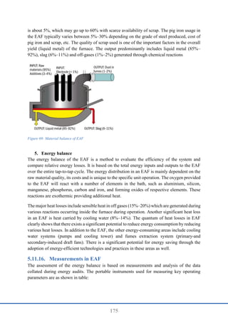
191. 177
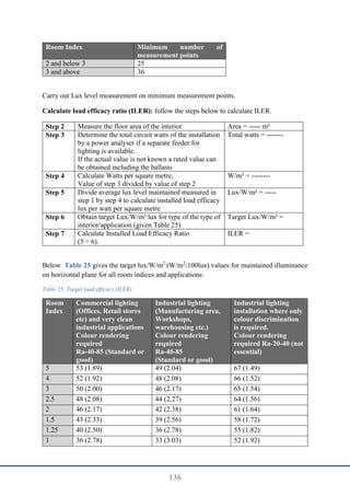
Heat in slag: The melting operation forms a sizeable quantity of slag. The slag comprises
oxides of Si, Mn, Ca, Fe, and Al along with other impurities present in charge material. This
slag is removed at very high temperatures leading to substantial heat losses.
Heat loss in slag = [m×Cp×L×(Tm-Ta)] +(m×L) + [m×Cp×L×(Ts-Tm)]
m: Quantity of slag (kg/heat)
Cps: Specific heat of solid slag (kcal/kg °C)
CpL: Specific heat of liquid slag (kcal/kg °C)
Tm: Melting point of slag
Ts: Temperature of slag (°C)
Ta: Ambient temperature (°C)
L: Heat required for phase transition (kCal/kg)
Heat losses through openings: Radiation and convection heat losses occur from openings
present in the furnace and through air infiltration due to furnace draft. The main opening in
furnace is slag door, which is kept open throughout the heat in most units.
Heat loss through opening =Fb ×E ×F ×A
E: Emissivity of the surface
Fb: Black body radiation at furnace temperature (kcal/kg/cm2
/hr)
F: Factor of radiation
A: Area of opening (cm2
)
Surface heat loss: The heat from furnace surfaces, such as sidewalls, roof, etc. are radiated to
the atmosphere. The quantum of surface heat losses are dependent on the type and quality of
insulation used in furnace construction. The surface heat loss per m2 area can be estimated
using:
Q = [a × (Ts–Ta)5/4] + [4.88 × E × {(Ts/100)4 – (Ta /100)4}]
a: Factor for direction of the surface of natural convection ceiling
TS: Surface temperature (K)
Ta: Ambient temperature (K)
E: Emissivity of external wall surface of the furnace
The total energy losses are the sum of all the losses occurring in the furnace.
Furnace efficiency: The efficiency of furnace is evaluated by subtracting various energy losses
from the total heat input. For this, various operating parameters pertaining to different heat
losses must be measured, for example, the energy consumption rate, heat generated from
chemical reactions, temperature of off-gases, surface temperatures, etc. Data for some of these
parameters can be obtained from production records while others must be measured with
special monitoring instruments.
Furnace efficiency = Total heat input – Total energy losses

192. 178
Energy savings opportunities in EAF
1. Replacement of old and inefficient power transformers in EAF units
The old (more than 20 years) and inefficient transformers with up to maximum power rating
of 500 kVA per tonne can be replaced with Ultra-high-power transformers (UHP) in EAF units,
which will help in reducing energy losses and shorter tap-to-tap time. This would help reduce
fixed losses of the EAF. By definition, in EAFs, if the input power is above 700 kVA per tonne,
the transformer is termed as UHP. Although UHPs are typically available in the range 700–
1,500 kVA.
2. Aluminium electrode arm
The electrode current-conducting arm carries power from the transformers to the electrodes. A
mild steel support with water-cooled copper cables is the standard material used in EAFs. A
copper clad, that is, steel arm with copper bus tubes, is also being used in the furnaces. The
copper system (Cu-system) has high strength and conductivity. The overall weight of the Cu-
system is quite high; the electromagnetic forces around the copper bus and electrode clamping
heads affect the system performance. This increases the system resistance leading to a drop in
the power fed to the furnace. The maintenance requirement for a Cu-system is also high.
The shortcomings in EAF operations with Cu-system can be overcome with ‘aluminium
electrode arm’. The aluminium system (Al-system) is lighter than the Cu-system which is also
a non-magnetic material. The Al-system comprises aluminium current conducting electrode
arms and columns with guide roll assemblies. The average energy savings with aluminium
electrode arm is estimated to be about 0.7%. The advantages of an Al-system include the
following:
 High-arc power
 Increased productivity
 Reduction in maintenance downtime
 Lower weight
 Less mechanical vibrations
3. Improved regulation control
One of the major issues with a conventional regulation system is that it is a complex-structure
contact on-load changer, which increases the switching time (3–5 seconds). Further, the on-
load changers operate in a high-intensity mode (frequent changes ~500–800 per day) leading
to high wear and tear thereby, decreasing the operational reliability.
The shortcomings in conventional regulation systems (analog/electro-hydraulic) can be
addressed with “high pressure hydraulic digital regulation”. The digital system would allow
minimum delays for switching from one melting stage to another. This system can be linked
with ‘Level-2 or 3’automation for dynamic production control. The main advantages of digital
based regulation system are the following:
 Reduction in tap-to-tap time
 Increase in productivity
 Increase in operational reliability

193. 179
4. Bottom stirring – inert gas purging
The molten metal in the arc furnace may not be of homogenous mass or uniform quality across
the cross section. This may result in increased tap-to-tap time and energy consumption.
Moreover, it can lead to a high rejection level. Homogenisation of the liquid metal bath is
required to overcome the issues and enhance productivity.
The bottom stirring of liquid bath in an EAF is a potential solution for better homogenisation
and ensures uniform quality. The mechanism used at present for bottom stirring is inert gas
injection, mostly used in developed countries. In an inert gas-stirring system, the stirring of
liquid metal is accomplished using inert gases such as argon or nitrogen. Bottom-stirring
systems based on inert gas injection are available either as a single tube or multi-hole plugs.
These plugs are either buried in the furnace hearth ramming mix or ‘indirect purging’ or in
contact with steel melt or ‘direct purging’. Indirect purging arrangement offers improved
stirring arrangement due to better distribution of inert gases.
The bottom stirring using inert gases are more suitable for smaller furnaces. Bottom stirring
further accelerates chemical reactions between steel and slag. The stirring helps in an increased
heat transfer with an estimated energy saving of 12–24 kWh per tonne liquid steel. It further
leads to increased metal yield of about 0.5%. However, the use of inert gas would require
significant maintenance after every heat. The advantages of inert gas-based bottom stirrer
include the following:
 Improved control of the temperature and chemical composition
 Lower consumption of refractory and electrode
 Shorter TTT times
 Improvement in liquid metal yield
5. Mist cooling for electrodes
Typically, graphite electrodes are used in EAFs. The electrodes are clamped by an electrode
holder and inserted in the furnace. The electric arc is generated between the tip of the electrodes
which produces heat to melt the material in the furnace. The side surface of the electrodes is
oxidised and consumed due to the high temperature. During the operation of the furnace, the
shape of electrodes changes and at the tip it decreases to as low as 70% of the original electrode
diameter.
The oxidation loss of the side surface of the electrodes can be reduced by coating the outer
surface or by reducing the outer surface temperature of the electrode. A jacket of water mist is
created over the outer surface of the electrodes which forms a coating over the electrodes
surface, thereby reducing the temperature of the side surface.

194. 180
Fuel Fired Furnace
Furnace oil is the major fuel used in oil fired furnaces, especially for reheating and heat
treatment of materials. Light diesel oil (LDO) is used in furnaces where presence of sulphur is
undesirable. The key to efficient furnace operation lies in complete combustion of fuel with
minimum excess air.
Furnaces operate with efficiencies as low as 7% as against up to 90% achievable in other
combustion equipment such as boiler. This is because of the high temperature at which the
furnaces have to operate to meet the required demand. For example, a furnace heating the stock
to 1200°C will have its exhaust gases leaving at least at 1200 °C resulting in a huge heat loss
through the stack.
However, improvements in efficiencies have been brought by methods such as preheating of
stock, preheating of combustion air and other waste heat recovery systems.
Instrument required (for fuel fired furnace)
 Flue gas analyser
 Thermal imaging camera
 IR thermometer
 Three-phase power analyser
 Digital distance operator
Performance terms for fuel fired furnace
𝑇ℎ𝑒𝑟𝑚𝑎𝑙 𝑒𝑓𝑓𝑖𝑐𝑖𝑒𝑛𝑐𝑦 𝑜𝑓 𝑡ℎ𝑒 𝑓𝑢𝑟𝑛𝑎𝑐𝑒 =
𝐻𝑒𝑎𝑡 𝑖𝑛 𝑡ℎ𝑒 𝑠𝑡𝑜𝑐𝑘
𝐻𝑒𝑎𝑡 𝑖𝑛 𝑡ℎ𝑒 𝑓𝑢𝑒𝑙 𝑐𝑜𝑛𝑠𝑢𝑚𝑒𝑑 𝑓𝑜𝑟 ℎ𝑒𝑎𝑡𝑖𝑛𝑔 𝑡ℎ𝑒 𝑠𝑡𝑜𝑐𝑘
𝑋 100
Performance evaluation of a typical fuel fired furnace
Thermal efficiency of process heating equipment, such as furnaces, ovens, heaters, or kilns is
the ratio of useful heat output to heat input.
In the context of performance assessment of furnaces, the concepts of excess air and
computation of various heat losses, as in case of boilers, could be applied, but there exist several
additionalities and features, that differentiate furnace efficiency from boiler efficiency.
Whereas boiler efficiency of 70-90% is achievable, furnace efficiencies at times are as low as
7%, while with favourable condition, like good design, appropriate loading, waste heat
recovery practices, efficiencies of up to 60% & higher can be achieved. The reasons for low
furnace efficiency include:
 High stack temperature and excess air levels.
 Low capacity utilization/ hearth loading.
 Radiation losses due to opening.
 Surface heat losses.
 Batch operation involving heating, cooling and soaking cycles.

195. 181
The purpose of a heating process is to introduce a certain amount of thermal energy into a
product, raising it to a certain temperature to prepare it for additional processing or change its
properties. To carry this out, the product is heated in a furnace. This results in energy losses in
different areas and forms as shown in Sankey diagram Figure 70 For most heating equipment,
a large amount of the heat supplied is wasted in the form of exhaust gases.
These furnace losses include:
 Heat storage loss in the furnace structure
 Losses from the furnace outside walls or structure
 Heat transported out of the furnace by the load conveyors, fixtures, trays, etc. called
material handling losses.
 Radiation losses from openings, hot exposed parts, etc.
 Heat carried by the cold air infiltration into the furnace
 Heat carried by the excess air used in the burners.
Figure 70: Furnace losses
Heat storage loss in the furnace structure: First, the metal structure and insulation of the
furnace must be heated so their interior surfaces are about the same temperature as the product
they contain. This stored heat is held in the structure until the furnace shuts down, then it leaks
out into the surrounding area. The more frequently the furnace is cycled from cold to hot and
back to cold again, the more frequently this stored heat must be replaced. Fuel is consumed
with no useful output.
Furnace wall losses: Wall or transmission losses are caused by the conduction of heat through
the walls, roof, and floor of the heating device, as shown in Figure 71 The wall losses continue
as long as the furnace is operating.

196. 182
Figure 71: Furnace wall losses
Radiation losses or opening losses: Furnaces and oven operating at temperatures above 540°C
might have significant radiation losses, as shown in Figure 72. Hot surfaces radiate energy to
nearby colder surfaces, and the rate of heat transfer increases with the fourth power of the
surface’s absolute temperature. If there are any openings, damaged roof/wall or open inspection
windows, there will be heat loss by radiation.
Figure 72: Furnace opening losses
Material handling losses: Many furnaces use equipment to convey the work into and out of
the heating chamber, and this can also lead to heat losses. Conveyor belts or product hangers
that enter the heating chamber cold and leave it at higher temperature drain energy from the
combustion gases. In car bottom furnaces, the hot car structure gives off heat to the room each
time it rolls out of the furnace to load or remove work. This lost energy must be replaced when
the car is returned to the furnace.

197. 183
Air infiltration: Excess air does not necessarily enter the furnace as part of the combustion air
supply. It can also infiltrate from the surrounding room if there is negative pressure in the
furnace. Because of the draft effect of hot furnace stacks, negative pressures are fairly common,
and cold air slips past leaky door seals, cracks and other openings in the furnace. Figure 73
illustrates air infiltration from outside the furnace. Every time the door is opened, considerable
amount of heat is lost. Economy in fuel can be achieved if the total heat that can be passed on
to the stock is as large as possible.
Waste-gas losses: Waste gas loss, also known as flue gas or stack loss, is made up of the heat
that cannot be removed from the combustion gases inside the furnace. The reason is the heat
flows from the higher temperature to the lower temperature heat receiver.
Furnace heat balance method
Heat balance helps us to numerically understand the present heat loss and efficiency and
improve the furnace operation using these data. Thus, preparation of heat balance is a pre-
requirement for assessing energy conservation potential. The methodology of a typical furnace
heat balance is given simultaneously along with an example in 5.11.26
The total heat input is provided in the form of fuel or power. The desired output is the heat
supplied for heating the material or process. Other heat outputs in the furnaces are undesirable
heat losses. The inputs and outputs are calculated on the basis of per tonne of stock/charge.
Similar to the method of evaluating boiler efficiency by indirect method, furnace efficiency
can also be calculated from heat balance. Furnace efficiency is calculated after subtracting
 sensible heat loss in flue gas
 loss due to moisture in flue gas
 heat loss due to openings in furnace
 heat loss through furnace skin and
 other unaccounted losses from the heat input to the furnace.
Figure 73: Air infiltration in furnace

198. 184
In order to carry out a heat balance, various parameters that are required are hourly oil
consumption, material output, excess air quantity, temperature of flue gas, temperature of
furnace at various zones, skin temperatures and hot combustion air temperature.
The energy absorbed by the material requires the use of specific heat which can be obtained
from reference manual/data book.
If the process requires a change in state, from solid to liquid, or liquid to gas, then in
addition to sensible heat, an additional quantity of energy is required called the latent heat of
fusion or latent heat of evaporation and this quantity of energy needs to be added to the total
energy requirement.
Measurement parameters in fuel fired furnace
The following are some of the key measurements to be carried out for the heat balance method
in reheating furnaces
 Weight of stock/billets heated, with the help of furnace operator obtain the weight of
stock or billets to be heated per batch.
 Using thermal imager camera or IR thermometer measure the initial and final
temperature of the stock/billets in °C
 Using thermal imager camera or IR thermometer measure temperature of the furnace
walls and roofs
 Using furnace engineering drawing which is usually available with engineering team,
find the area of furnace walls and roof
 Using flue gas analyser, measure the flue gas temperature
 Using the flue gas analyser, measure the O2, CO2, CO (and other gas) parameters
 Measure or collect from industry measured values of the fuel consumption of furnace
per batch
 Reference manual shall be referred for certain data like specific heat and humidity, etc.
Determine fuel fire furnace efficiency by direct method
The direct determination of furnace efficiency is carried out as follows:
𝑇ℎ𝑒𝑟𝑚𝑎𝑙 𝑒𝑓𝑓𝑖𝑐𝑖𝑒𝑛𝑐𝑦 𝑜𝑓 𝑡ℎ𝑒 𝑓𝑢𝑟𝑛𝑎𝑐𝑒 =
𝐻𝑒𝑎𝑡 𝑖𝑛 𝑡ℎ𝑒 𝑠𝑡𝑜𝑐𝑘
𝐻𝑒𝑎𝑡 𝑖𝑛 𝑡ℎ𝑒 𝑓𝑢𝑒𝑙 𝑐𝑜𝑛𝑠𝑢𝑚𝑒𝑑 𝑓𝑜𝑟 ℎ𝑒𝑎𝑡𝑖𝑛𝑔 𝑡ℎ𝑒 𝑠𝑡𝑜𝑐𝑘
𝑋 100
Heat in the stock can be found by following formula:
Qs = m X Cp X (t2 – t1)
Where,
m = weight of the stock in kg
Cp = Specific heat of stock in kcal/kg°C
t1 = final temperature of stock desired in °C
t2 = Initial temperature of stock before it enters the furnace in °C

199. 185
And, Heat in the fuel consumed for heating the stock can be found by following formula:
Heat in Fuel = Quantity of fuel X gross calorific value (GCV) of fuel
Example: the following are the operating parameters of rerolling mill furnace
Weight of input material – 10 t/hr
Furnace oil consumption – 600 l/hr
Specific gravity of oil – 0.92
Final material temperature - 1200°C
Initial material temperature - 40°C
Specific heat of the material – 0.12 kcal/kg/°C
GCV of oil – 10,000 kcal/kg
Yield percentage of furnace – 92%
a. Calculate furnace efficiency by direct method
b. Calculate specific fuel consumption on finished based basis
Solution:
a. Furnace efficiency by direct method
Heat input = 600 l/hr X 0.92 X 10,000 = 55,20,000 kcal/hr
Heat output = 10,000 X 0.12 X (1200 – 40) = 13,92,000 kcal/hr
Efficiency = 13,92,000 / 55,20,000 = 25.2%
b. Specific fuel consumption of finished basis
Weight of finished products = 10 X 0.92 = 9.2 t/hr
Furnace oil consumption = 600 l/hr
Specific fuel consumption = 660/9.2 = 65.2 l/t

200. 186
Example: Heat balance of furnace
An oil-fired reheating furnace has an operating temperature of 1340°C. Average fuel
consumption is 400 l/hr. The flue gas exit temperature after air pre-heater is 655°C. Air is pre-
heated from ambient temperature of 40°C to 190°C through an air pre-heater. The furnace has
460 mm thick wall on the billet extraction outlet side, which is 1mm high (D) and 1 m wide.
Draw a heat balance to identify losses, efficiency and specific fuel consumption. The other data
are as follows:
Parameter Value
Flue gas temperature after air pre-heater 655°C
Ambient temperature 40°C
Absolute humidity 0.03437 kg/kg dry air
Pre-heated air temperature 190°C
Specific gravity of oil 0.92
Average fuel oil consumption (l/hr) 400 l/hr
Average fuel oil consumption (kg/hr) = 400 X 0.92 = 368 kg/hr
O2 in flue gas 12%
CO2 in flue gas 6.5%
CO in flue gas 50 ppm
Weight of stock 6,000 kg/hr
Specific heat of billet 0.12 kcal/kg°C
Surface temperature of ceiling 85°C
Surface temperature of side walls 100°C
Surface temperature of flue duct 64°C
Area of ceiling 15 m2
Area of side walls 36 m2
Area of flue duct 10.3 m2
Diameter of flue duct 0.4 m
Furnace oil constituents (% by weight)
Carbon: 85.9%, Hydrogen: 12%, Oxygen: 0.7%, Nitrogen: 0.5%, Sulphur: 0.5%, H2O: 0.35%,
Ash: 0.05%, GCV: 10,000 kcal/kg

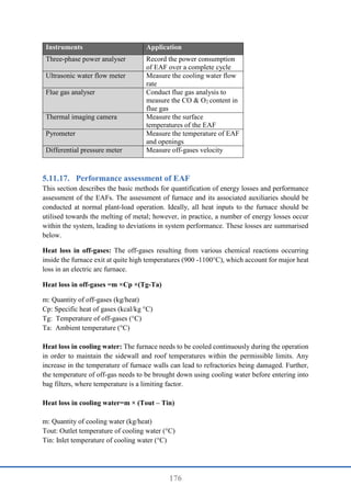
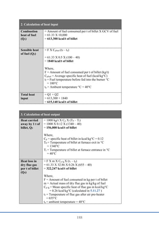
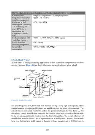
201. 187
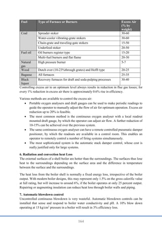
Solution:
1.Calculation of air quantity and specific fuel consumption
Theoretical air
required for
combustion
[(11.6 X C) + {34.8 X (H2 – O2/8)} + (4.35 X S)] / 100 kg/kg
of fuel (from fuel analysis)
= [(11.6 X 85.9) + {34.8 x (12-0.7/8)} + (4.35 X 0.5)] /100
= 14.12 kg of air/kg of fuel
% excess air
supplied (EA) =
𝑂2%
21 − 𝑂2%
𝑋 100 =
12
21 − 12
𝑋 100 = 𝟏𝟑𝟑. 𝟑%
Actual mass of
air supplied / kg
of fuel (AAS)
= (1 +
𝐸𝐴
100
) 𝑋 𝑡ℎ𝑒𝑜𝑟𝑒𝑡𝑖𝑐𝑎𝑙 𝑎𝑖𝑟
= (1 +
133.3
100
) 𝑋 14.12 = 𝟑𝟐. 𝟗𝟒 𝒌𝒈 𝒐𝒇𝒂𝒊𝒓/𝒌𝒈 𝒐𝒇 𝒇𝒖𝒆𝒍
Mass of dry flue
gas (md)
= Mass of CO2 + Mass of N2 content in the fuel + Mass of
sulphur dioxide + Mass of N2 in the combustion air supplied +
Mass of oxygen in flue gas
=
0.859 𝑋 44
12
+ 0.005 +
0.005 𝑋 64
32
+
32.94 𝑋 77
100
+
(32.94 − 141.12) 𝑋 23
100
= 32.86 kg/kg of coal
Amount of wet
flue gas
= AAS +1 = 32.94 + 1
= 33.94 kg of flue gas / kg of fuel
Amount of water
vapor in flue gas
(mw)
= M + 9 H2 (M - % moisture in fuel, H2 - % hydrogen in fuel)
= (0.35/100) + 9 x (12/100)
= 1.084 kg of H2O/kg of fuel
Amount of dry
flue gas
Amount of wet flue gas -Amount of water vapour in flue gas
= 33.94-1.084
= 32.86 kg /kg of fuel
Specific fuel
consumption
= Amount of fuel consumed (kg/hr) / Amount of billet (t/hr)
= 368 /6
= 61.33 kg of fuel / t of billet

202. 188
2. Calculation of heat input
Combustion
heat of fuel
(Q1)
= Amount of fuel consumed per t of billet X GCV of fuel
= 61.33 X 10,000
= 613,300 kcal/t of billet
Sensible heat
of fuel (Q2)
= F X Cpfuel (tf – ta)
= 61.33 X 0.5 X (100 – 40)
= 1840 kcal/t of billet
Where,
F = Amount of fuel consumed per t of billet (kg/t)
Cpfuel = Average specific heat of fuel (kcal/kg°C)
tf = Fuel temperature before fed into the burner °C
= 100°C
ta = Ambient temperature °C = 40°C
Total heat
input
= Q1 + Q2
= 613,300 + 1840
= 615,140 kcal/t of billet
3. Calculation of heat output
Heat carried
away by 1 t of
billet, Q3
= 1000 kg/t X Cp X (T0 – Ti)
= 1000 X 0.12 X (1340 – 40)
= 156,000 kcal/t of billet
Where,
Cp = specific heat of billet in kcal/kg°C = 0.12
T0 = Temperature of billet at furnace exit in °C
= 1340°C
Ti = Temperature of billet at furnace entrance in °C
= 40°C
Heat loss in
dry flue gas
per t of billet
(Q4)
= F X m X Cp fg X (t1 – ta)
= 61.33 X 32.86 X 0.26 X (655 – 40)
= 322,247 kcal/t of billet
Where,
F = Amount of fuel consumed in kg per t of billet
m = Actual mass of dry flue gas in kg/kg of fuel
Cp fg = Mean specific heat of flue gas in kcal/kg°C
= 0.26 kcal/kg°C (calculated in 5.11.27 )
t1 = Temperature of flue gas after air pre-heater
= 655°C
ta = ambient temperature = 40°C

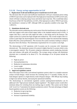
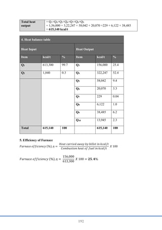
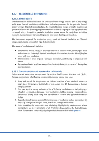
203. 189
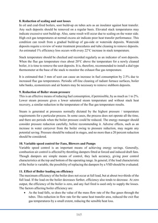
3. Calculation of heat output
Heat loss due
to formation
of water
vapour from
fuel per t of
billet (Q5)
= F X mw X (584 + Cp of super-heated vapor X (t1 – ta))
= 61.33 X 1.084 X (584 + 0.47 X (655 – 40)
= 58,042 kcal/t of billet
Where,
mw = amount of water vapour in flue gas
Cp of super-heated vapor (for specific heat value refer Table 36)
Heat loss due
to moisture in
combustion
air (Q6)
= F X AAS X humidity of air X Cp of super-heated vapor X (t1 –
ta))
= 61.33 X 32.94 X 0.03437 X 0.47 X (655 – 40)
= 20,070 kcal/t of billet
Heat loss due
to partial
conversion of
C to CO (Q7)
= 𝐹 𝑋
%𝐶𝑂 𝑋 𝐶
%𝐶𝑂+%𝐶𝑂2
𝑋 5654
= 61. 33𝑋
0.005 𝑋 0.859
0.005+6.5
𝑋 5654
= 229 kcal/t of billet
Amount of
heat loss from
the furnace
body and
other sections
(Q8)
Where,
= (q1 +q2 + q3 + q4), kcal/hr / amount of billet (t/hr)
Where,
q1 = Heat loss from the furnace body ceiling surface
(horizontal surface facing upward)
q2 = Heat loss from the furnace body sidewall surface
(vertical surfacing sideways)
q3 = Bottom (horizontal surface facing downward)
q4 = Heat loss from the flue gas duct between the furnace
exit and air pre-heater (including heat loss from the
external surface of the air pre-heater)
q1
= [ℎ 𝑋 𝐴 𝑋 (𝑡1 − 𝑡2)1.25
] + [4.88 𝑋 𝐸 𝑋 (
𝑡1+273
100
)
4
−
(
𝑡2+273
100
)
4
𝑋 𝐴]
= [2.8 𝑋 15 𝑋 (85 − 40)1.25] +
[4.88 𝑋 0.75 𝑋 (
85+273
100
)
4
− (
40+273
100
)
4
𝑋 15]
= [2.8 X 15 X 451.25
] + [4.88 X 0.75 X (3.58)4
– (3.13)4
X
15
= 8,644 kcal/hr
Where,

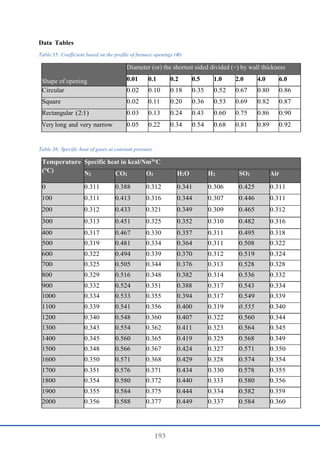
204. 190
3. Calculation of heat output
h = heat rate, natural convection factor, (for ceiling = 2.8
kcal/m2h°C)
A = ceiling surface area (m2
) = 15 m2
t1 = External temperature of ceiling = 85°C
t2 = Ambient temperature around furnace = 40°C
E = Emissivity of the furnace body surface = 0.75
q2
= [ℎ 𝑋 𝐴 𝑋 (𝑡1 − 𝑡2)1.25
] + [4.88 𝑋 𝐸 𝑋 (
𝑡1+273
100
)
4
−
(
𝑡2+273
100
)
4
𝑋 𝐴]
= [2.2 𝑋 36 𝑋 (100 − 40)1.25] +
[4.88 𝑋 0.75 𝑋 (
100+273
100
)
4
− (
40+273
100
)
4
𝑋 36]
= [2.2 X 36 X 601.25
] + [4.88 X 0.75 X (3.73)4
– (3.13)4
X
36]
= 26,084 kcal/hr
Where,
h = heat rate, natural convection factor, (for sidewall = 2.2
kcal/m2h°C)
A = side wall surface area (m2
) = 36 m2
t1 = External temperature of sidewall = 100°C
t2 = Ambient temperature around furnace = 40°C
E = Emissivity of the furnace body surface = 0.75
q3 = Bottom (horizontal surface facing downward)
As the bottom surface is not exposed to the atmosphere q3
is ignored in this calculation
q4
= [ ℎ 𝑋 𝐴 𝑋
(𝑡1−𝑡2)1.25
𝐷0⋅25
] + [4.88 𝑋 𝐸 𝑋 (
𝑡1+273
100
)
4
−
(
𝑡2+273
100
)
4
𝑋 𝐴]
= [ 1.1 𝑋 10.3 𝑋
(64−40)1.25
0.40⋅25
] +
[4.88 𝑋 0.75 𝑋 (
64+273
100
)
4
− (
40+273
100
)
4
𝑋 10.3]
= [1.1 X 10.3 X (41.25
/0.40.25
)] + [4.88 X 0.75 X (3.37)4
–
(3.13)4
X 10.3]
= 2,001 kcal/hr
h = heat rate, natural convection factor, (for flue gas duct =
1.1 kcal/m2
h°C)

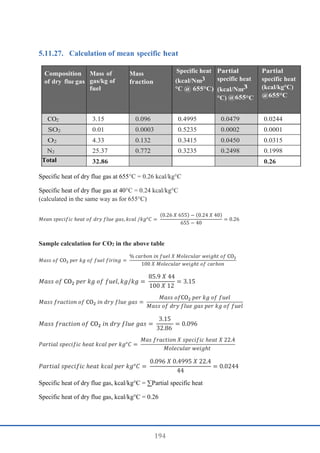
205. 191
3. Calculation of heat output
A = External surface area of flue gas duct (m2
) =10.3 m2
D = Outside diameter of the flue gas duct in m = 0.4 m
t1 = External temperature of flue gas duct = 64°C
t2 = Ambient temperature around furnace = 40°C
E = Emissivity of the furnace body surface = 0.75
Q8 = (q1 + q2 +q3 +q4) / amount of billet (t/hr)
= 8,644 + 26,084 +0 + 2,001
= 6,122 kcal/t
Radiation
heat loss
through
furnace
openings (Q9)
= ℎ𝑟 𝑋 𝐴 𝑋 𝛷 𝑋 4.88 𝑋 [(
𝑡1+273
100
)
4
− (
𝑡2+273
100
)
4
] / amount
of billet (t/hr)
= 1 𝑋 1 𝑋 0.70 𝑋 4.88 𝑋 [(
1613
100
)
4
− (
313
100
)
4
] /6
= 38,485 kcal/t
Where,
hr = open time during the period of heat balancing =1 hr
A = Area of an opening in m2
= 1 m2
Φ = Co-efficient based on the profile of furnace openings
(from Table 35)
= Diameter (or) the shortest side / wall thickness
= 1/0.46 = 2.17
= 0.70 (value corresponding to 2.17 and square shape from
Table 35)
t1= furnace temperature = 1340°C
t2= ambient temperature around furnace = 40°C
Amount of billet (t/hr) = 6
Other types of
heat loss /
unaccounted
losses (Q10)
other types of heat loss will include the following,
 Heat carried away cooling water in the flue damper
 Heat carried away by cooling water at the furnace access door
 Radiation from the furnace bottom
 Heat accumulated by refractory
 Instrumental error and measuring error
 Others
Q10 = Q1+Q2 – (Q3+Q4+Q5+Q6+Q7+Q8+Q9)
= (6,13,300 + 1,840) – (1,56,000 + 3,22,247 + 58,042 + 20,070 +229
+ 6,122 + 38,485)
= 13,945 kcal/t

206. 192
Total heat
output
= Q3+Q4+Q5+Q6+Q7+Q8+Q9
= 1,56,000 + 3,22,247 + 58,042 + 20,070 +229 + 6,122 + 38,485
= 615,140 kcal/t
4. Heat balance table
Heat Input Heat Output
Item kcal/t % Item kcal/t %
Q1 613,300 99.7 Q3 156,000 25.4
Q2 1,840 0.3 Q4 322,247 52.4
Q5 58,042 9.4
Q6 20,070 3.3
Q7 229 0.04
Q8 6,122 1.0
Q9 38,485 6.2
Q10 13,945 2.3
Total 615,140 100 615,140 100
5. Efficiency of Furnace
𝐹𝑢𝑟𝑛𝑎𝑐𝑒 𝑒𝑓𝑓𝑖𝑐𝑖𝑒𝑛𝑐𝑦 (%), 𝜂 =
𝐻𝑒𝑎𝑡 𝑐𝑎𝑟𝑟𝑖𝑒𝑑 𝑎𝑤𝑎𝑦 𝑏𝑦 𝑏𝑖𝑙𝑙𝑒𝑡 𝑖𝑛 𝑘𝑐𝑎𝑙/𝑡
𝐶𝑜𝑚𝑏𝑢𝑠𝑡𝑖𝑜𝑛 ℎ𝑒𝑎𝑡 𝑜𝑓 𝑓𝑢𝑒𝑙 𝑖𝑛 𝑘𝑐𝑎𝑙/𝑡
𝑋 100
𝐹𝑢𝑟𝑛𝑎𝑐𝑒 𝑒𝑓𝑓𝑖𝑐𝑖𝑒𝑛𝑐𝑦 (%), 𝜂 =
156,000
613,300
𝑋 100 = 𝟐𝟓. 𝟒%

207. 193
Data Tables
Table 35: Coefficient based on the profile of furnace openings (Φ)
Shape of opening
Diameter (or) the shortest sided divided (÷) by wall thickness
0.01 0.1 0.2 0.5 1.0 2.0 4.0 6.0
Circular 0.02 0.10 0.18 0.35 0.52 0.67 0.80 0.86
Square 0.02 0.11 0.20 0.36 0.53 0.69 0.82 0.87
Rectangular (2:1) 0.03 0.13 0.24 0.43 0.60 0.75 0.86 0.90
Very long and very narrow 0.05 0.22 0.34 0.54 0.68 0.81 0.89 0.92
Table 36: Specific heat of gases at constant pressure
Temperature
(°C)
Specific heat in kcal/Nm3°C
N2 CO2 O2 H2O H2 SO2 Air
0 0.311 0.388 0.312 0.341 0.306 0.425 0.311
100 0.311 0.413 0.316 0.344 0.307 0.446 0.311
200 0.312 0.433 0.321 0.349 0.309 0.465 0.312
300 0.313 0.451 0.325 0.352 0.310 0.482 0.316
400 0.317 0.467 0.330 0.357 0.311 0.495 0.318
500 0.319 0.481 0.334 0.364 0.311 0.508 0.322
600 0.322 0.494 0.339 0.370 0.312 0.519 0.324
700 0.325 0.505 0.344 0.376 0.313 0.528 0.328
800 0.329 0.516 0.348 0.382 0.314 0.536 0.332
900 0.332 0.524 0.351 0.388 0.317 0.543 0.334
1000 0.334 0.533 0.355 0.394 0.317 0.549 0.339
1100 0.339 0.541 0.356 0.400 0.319 0.555 0.340
1200 0.340 0.548 0.360 0.407 0.322 0.560 0.344
1300 0.343 0.554 0.362 0.411 0.323 0.564 0.345
1400 0.345 0.560 0.365 0.419 0.325 0.568 0.349
1500 0.348 0.566 0.367 0.424 0.327 0.571 0.350
1600 0.350 0.571 0.368 0.429 0.328 0.574 0.354
1700 0.351 0.576 0.371 0.434 0.330 0.578 0.355
1800 0.354 0.580 0.372 0.440 0.333 0.580 0.356
1900 0.355 0.584 0.375 0.444 0.334 0.582 0.359
2000 0.356 0.588 0.377 0.449 0.337 0.584 0.360

208. 194
Calculation of mean specific heat
Composition
of dry flue gas
Mass of
gas/kg of
fuel
Mass
fraction
Specific heat
(kcal/Nm3
°C @ 655°C)
Partial
specific heat
(kcal/Nm3
°C) @655°C
Partial
specific heat
(kcal/kg°C)
@655°C
CO2 3.15 0.096 0.4995 0.0479 0.0244
SO2 0.01 0.0003 0.5235 0.0002 0.0001
O2 4.33 0.132 0.3415 0.0450 0.0315
N2 25.37 0.772 0.3235 0.2498 0.1998
Total 32.86 0.26
Specific heat of dry flue gas at 655°C = 0.26 kcal/kg°C
Specific heat of dry flue gas at 40°C = 0.24 kcal/kg°C
(calculated in the same way as for 655°C)
𝑀𝑒𝑎𝑛 𝑠𝑝𝑒𝑐𝑖𝑓𝑖𝑐 ℎ𝑒𝑎𝑡 𝑜𝑓 𝑑𝑟𝑦 𝑓𝑙𝑢𝑒 𝑔𝑎𝑠, 𝑘𝑐𝑎𝑙 /𝑘𝑔°𝐶 =
(0.26 𝑋 655) − (0.24 𝑋 40)
655 − 40
= 0.26
Sample calculation for CO2 in the above table
𝑀𝑎𝑠𝑠 𝑜𝑓 CO2 𝑝𝑒𝑟 𝑘𝑔 𝑜𝑓 𝑓𝑢𝑒𝑙 𝑓𝑖𝑟𝑖𝑛𝑔 =
% 𝑐𝑎𝑟𝑏𝑜𝑛 𝑖𝑛 𝑓𝑢𝑒𝑙 𝑋 𝑀𝑜𝑙𝑒𝑐𝑢𝑙𝑎𝑟 𝑤𝑒𝑖𝑔ℎ𝑡 𝑜𝑓 CO2
100 𝑋 𝑀𝑜𝑙𝑒𝑐𝑢𝑙𝑎𝑟 𝑤𝑒𝑖𝑔ℎ𝑡 𝑜𝑓 𝑐𝑎𝑟𝑏𝑜𝑛
𝑀𝑎𝑠𝑠 𝑜𝑓 CO2 𝑝𝑒𝑟 𝑘𝑔 𝑜𝑓 𝑓𝑢𝑒𝑙, 𝑘𝑔/𝑘𝑔 =
85.9 𝑋 44
100 𝑋 12
= 3.15
𝑀𝑎𝑠𝑠 𝑓𝑟𝑎𝑐𝑡𝑖𝑜𝑛 𝑜𝑓 CO2 𝑖𝑛 𝑑𝑟𝑦 𝑓𝑙𝑢𝑒 𝑔𝑎𝑠 =
𝑀𝑎𝑠𝑠 𝑜𝑓CO2 𝑝𝑒𝑟 𝑘𝑔 𝑜𝑓 𝑓𝑢𝑒𝑙
𝑀𝑎𝑠𝑠 𝑜𝑓 𝑑𝑟𝑦 𝑓𝑙𝑢𝑒 𝑔𝑎𝑠 𝑝𝑒𝑟 𝑘𝑔 𝑜𝑓 𝑓𝑢𝑒𝑙
𝑀𝑎𝑠𝑠 𝑓𝑟𝑎𝑐𝑡𝑖𝑜𝑛 𝑜𝑓 CO2 𝑖𝑛 𝑑𝑟𝑦 𝑓𝑙𝑢𝑒 𝑔𝑎𝑠 =
3.15
32.86
= 0.096
𝑃𝑎𝑟𝑡𝑖𝑎𝑙 𝑠𝑝𝑒𝑐𝑖𝑓𝑖𝑐 ℎ𝑒𝑎𝑡 𝑘𝑐𝑎𝑙 𝑝𝑒𝑟 𝑘𝑔°𝐶 =
𝑀𝑎𝑠 𝑓𝑟𝑎𝑐𝑡𝑖𝑜𝑛 𝑋 𝑠𝑝𝑒𝑐𝑖𝑓𝑖𝑐 ℎ𝑒𝑎𝑡 𝑋 22.4
𝑀𝑜𝑙𝑒𝑐𝑢𝑙𝑎𝑟 𝑤𝑒𝑖𝑔ℎ𝑡
𝑃𝑎𝑟𝑡𝑖𝑎𝑙 𝑠𝑝𝑒𝑐𝑖𝑓𝑖𝑐 ℎ𝑒𝑎𝑡 𝑘𝑐𝑎𝑙 𝑝𝑒𝑟 𝑘𝑔°𝐶 =
0.096 𝑋 0.4995 𝑋 22.4
44
= 0.0244
Specific heat of dry flue gas, kcal/kg°C = ∑Partial specific heat
Specific heat of dry flue gas, kcal/kg°C = 0.26

209. 195
Energy savings opportunities in fuel fired furnaces
1. Excess air optimization
The quantum of waste heat generation is directly proportional to the quantity of air used for
combustion of fuel. Air, slightly in excess of ideal stoichiometric (or theoretical) is required
(air ratio) for complete combustion. However, excess air beyond optimum range may
substantially decrease combustion efficiency as it leads to generation of excessive hot waste
gases. On the other hand, if the excess air is less, then unburnt components in flue gases will
increase and would be carried away in the flue gases through stack. The optimization of
combustion air is the most attractive and economical measure for energy conservation. The
impact of this measure is higher when the temperature of furnace is high.
Air Ratio is defined as the ratio of “actual air supplied” (AAS) to theoretical air requirement.
The following formula shall be used for calculating the air ratio (value rounded to two digits).
The air ratio is considered based on steady state operation at constant load conditions and can
be measured and verified at specific measurement points while maintaining maximum
permissible limit for carbon monoxide (CO) level to 200 ppm.
𝐴𝑖𝑟 𝑟𝑎𝑡𝑖𝑜 =
21
21 − 𝑂𝑥𝑦𝑔𝑒𝑛 % 𝑖𝑛 𝑓𝑙𝑢𝑒 𝑔𝑎𝑠
 Using a flue gas analyser, measure the oxygen % in flue gas
 Maintain the air ratio for industrial fuel fired furnaces as per below Table 37
Table 37: Air ratio for fuel fired furnaces
Kiln type Air ratio for oil
fired furnaces
Oxygen% in flue
gas
Oil heating (thermal
fluid heater)
1.18 – 1.22 3.2% - 3.7%
Reheating Furnace 1.15 – 1.20 2.73% - 3.5%
2. Air ratio control by VFD
Controlling oxygen levels and using Variable frequency Drives (VFDs) on combustion air
fans associated with reheating furnaces help in optimizing combustion in the furnace. The use
of VFDs on combustion air fans in reheating furnace also helps to control oxygen levels,
especially during variation in furnace production rate. The fuel and electricity savings in
reheating furnace through optimization of excess air level depend on load factor of the furnace
and the control strategies applied. The estimated energy saving is 4%–9% of thermal energy.
3. Air ratio control by damper
If a reheating furnace is not equipped with an automatic air ratio fuel controller, it is necessary
to periodically sample gas in the furnace and measure its oxygen contents by a flue gas analyser
and accordingly adjust the damper to control and maintain the target air fuel ratio.

210. 196
4. Uniform heat distribution
Furnace design should be such that in a given time, as much of the stock could be heated
uniformly to a desired temperature with minimum fuel firing rate.
Following points shall be examined during audit for furnace burners:
 The flame should not touch any solid object and should propagate clear of any solid
object. Any obstruction will atomise the fuel particles thus affecting combustion and
create black smoke. If flame impinges on the stock, there would be increase in scale
losses. (Refer Figure 74 to Figure 77)
 If the flames impinge on refractories, the incomplete combustion products can settle
and react with refractory constituents at high flame temperatures.
 The flames of different burners in a furnace should stay clear of each other. If they
intersect, inefficient combustion will occur. It is recommended to stagger the burners
on the opposite sides.
 The burner flame tends to travel freely in the combustion space just above the material.
In small furnaces, the axis of the burner is never placed parallel to the hearth but always
at an upward angle. Flame should not hit the roof.
 The larger burners produce a long flame, which may be difficult to contain within the
furnace walls. More burners of less capacity give better heat distribution in the furnace
and also increase furnace life.
 For small furnaces, it is desirable to have a long flame with golden yellow colour while
firing furnace oil for uniform heating. The flame should not be too long that it enters
the chimney or comes out through the furnace top or through doors. In such cases, major
portion of additional fuel is carried away from the furnace.
Figure 74: Wrong Correct heat
distribution in furnace
Figure 75: Correct heat
distribution in furnace
Figure 76: Wrong alignment of
burners
Figure 77: Correct alignment of
burners

211. 197
5. Maintaining optimum operating temperature of furnace
It is important to operate the furnace at optimum temperature. The operating temperature of
various furnaces are given in below Table 38
Table 38: Operating temperature of various furnaces
Operating temperature of various furnaces
Slab reheating furnaces 1200°C
Rolling mill furnaces 1200°C
Bar furnace for sheet mill 800°C
Bogey type annealing furnace 650 - 750°C
Operating at too high temperatures than optimum causes heat loss, excessive oxidation,
decarbonisation as well as over stressing of the refractories. These controls are normally left to
operator judgement, which is not desirable. To avoid human error, on/off controls should be
provided.
6. Prevention of heat loss through openings
Heat loss through openings consists of, the heat loss by direct radiation through openings
plus(+) the heat loss caused by combustion gas that leaks through openings, If the furnace
pressure is slightly higher than outside air pressure (as in case of reheating furnace) during its
operation, the combustion gas inside may blow off through openings and results in heat loss.
But it is more detrimental, if outside air intrudes into the furnace, creating uneven temperature
distribution inside the furnace and in process also oxidizing billets.
7. Control of furnace draft
If negative pressures exist in the furnace, air infiltration is liable to occur through the cracks
and openings thereby affecting air- fuel ratio control. Tests conducted on apparently airtight
furnaces have shown air infiltration up to the extent of 40%. Neglecting furnaces pressure could
mean problems of cold metal and non-uniform metal temperatures, which could affect
subsequent operations like forging and rolling and result in increased fuel consumption. For
optimum fuel consumption, slight positive pressure should be maintained in the furnace as
shown in Figure 78 Exfiltration is less serious than infiltration. Some of the associated
problems with exfiltration are leaping out of flames, overheating of the furnace refractories
leading to reduced brick life, increased furnace maintenance, burning out of ducts and
equipment attached to the furnace.

212. 198
Figure 78: Effect of pressure on the location of zero level and infiltration of air (Source: BEE)
In addition to the proper control on furnace pressure, it is important to keep the openings as
small as possible and to seal them in order to prevent the release of high temperature gas and
intrusion of outside air through openings such as the charging inlet, extracting outlet and
peephole on furnace walls or the ceiling.
8. Optimum capacity utilisation
One of the most vital factors affecting efficiency is loading. There is a specific loading at
which the furnace will operate at maximum thermal efficiency. If the furnace is under loaded
a smaller fraction of the available heat in the working chamber will be taken up by the load and
therefore efficiency will be low.
The best method of loading is generally obtained by trial; note the weight of material put in at
each charge, the time it takes to reach the desired temperature and the amount of fuel used.
Every endeavour should be made to load a furnace at the rate associated with optimum
efficiency although it must be realised that limitations to achieving this are sometimes imposed
by work availability or other factors beyond control.
The loading of the charge on the furnace hearth should be arranged so that
 It receives the maximum amount of radiation from the hot surfaces of the heating
chambers and the flames produced.
 The hot gases are efficiently circulated around the heat receiving surfaces
Stock should not be placed in the following position
 In the direct path of the burners or where flame impingement is likely to occur
 In an area which is likely to cause a blockage or restriction of the flue system of the
furnace.
 Close to any door openings where cold spots are likely to develop.
In the interests of economy and work quality the materials comprising the load should only
remain in the furnace for the minimum time to obtain the required physical and metallurgical

213. 199
requirements. When the materials attain these properties, they should be removed from the
furnace to avoid damage and fuel wastage. The higher the working temperature, higher is the
loss per unit time. The effect on the materials by excessive residence time will be an increase
in surface defects due to oxidation. The rate of oxidation is dependent upon time, temperature,
as well as free oxygen content. The possible increase in surface defects can lead to rejection
of the product. It is therefore essential that coordination between the furnace operator,
production and planning personnel be maintained. One of the reasons for not operating the
furnace at optimum loading is the mismatching of furnace dimension with respect to charge
and production schedule.
9. Waste heat recovery from furnace flue gases
In any industrial furnace the products of combustion leave the furnace at a temperature higher
than the stock temperature. Sensible heat losses in the flue gases, while leaving the chimney
carry 35 to 55% of the heat input to the furnace. The higher the quantum of excess air and flue
gas temperature, the higher would be the waste heat availability. Waste heat recovery should
be considered after all other energy conservations measures have been taken. Minimising the
generation of waste heat should be the primary objective.
The sensible heat in flue gases can be generally recovered by the following methods:
 Charge (stock) preheating
 Preheating of combustion air
 Utilising waste heat for other process (to generate steam or hot water by a waste heat
boiler)
Charge pre-heating
When raw materials are preheated by exhaust gases before being placed in a heating furnace,
the amount of fuel necessary to heat them in the furnace is reduced. Since raw materials are
usually at room temperature, they can be heated sufficiently using high temperature to reduce
fuel consumption.
Preheating of combustion air
The energy contained in the exhaust gases can be recycled by using it to pre-heat the
combustion air. A variety of equipment is available to preheat the combustion air such as:
Radiation recuperators generally, take the form of concentric cylinders, in which the
combustion air passes through the annulus and the exhaust gases from the furnace pass through
the centre, see Figure 79 (a). The simple construction means that such recuperators are suitable
for use with dirty gases, have a negligible resistance to flow, and can replace the flue or
chimney if space is limited. The annulus can be replaced by a ring of vertical tubes, but this
design is more difficult to install and maintain. Radiation recuperators rely on radiation from
high temperature exhaust gases and should not be employed with exhaust gases at less than
about 800°C.

214. 200
Convection recuperators consist essentially of bundles of drawn or cast tubes; see Figure 79
(b) Internal and/or external fins can be added to assist heat transfer. The combustion air
normally passes through the tubes and the exhaust gases outside the tubes, but there are some
applications where this is reversed. For example, with dirty gases, it is easier to keep the tubes
clean if the air flows on the outside. Design variations include 'U' tube and double pass systems.
Convection recuperators are more suitable for exhaust gas temperatures of less than about
900°C.
Self-Recuperative burners are based on traditional heat recovery techniques in that the
products of combustion are drawn through a concentric tube recuperator around the burner
body and used to pre-heat the combustion air. A major advantage of this type of system is that
it can be retrofitted an existing furnace structure to increase production capability without
having to alter the existing exhaust gas ducting arrangements. Self-recuperative burners are
generally more suited to heat treatment furnaces where exhaust gas temperatures are lower and
there are no stock recuperation facilities.
Figure 79: Recuperators
Estimation of fuel savings by pre-heating combustion air: By using preheated air for
combustion, fuel can be saved. The fuel saving rate is given by the following formula:
𝑆 =
𝑃
𝐹 + 𝑃 − 𝑄
𝑋 100
Where, S: Fuel saving rate (%)
F: Calorific value of fuel (kcal/kg fuel)
P: Quantity of heat brought in by preheated air (kcal/kg fuel)
Q: Quantity of heat taken away by exhaust gas (kcal/kg)
By this formula, fuel savings rates for heavy oil were calculated for various temperatures of
exhaust gas and preheated air. The results are shown in the following Figure 80

215. 201
Figure 80: Fuel savings rate by preheated air temperature (Source: BEE)
For example, when combustion air for heavy oil is preheated to 400°C by a heat exchanger
with an inlet temperature of 800 °C, the fuel conservation rate is estimated to be about 20
percent. When installing a recuperator in a continuous steel reheating furnace, it is important
to choose a preheated air temperature that will balance the fuel saving effect and the invested
cost for the equipment.
Also, the following points should be checked:
Draft of exhaust gas: When exhaust gas goes through a recuperator, its draft resistance usually
causes a pressure loss of 5-10 mm H2O.Thus, the draft of stack should be checked.
Air blower for combustion air: While the air for combustion goes through a recuperator,
usually 100-200 mm H2O pressure is lost. Thus, the discharge pressure of air blower should be
checked, and the necessary pressure should be provided by burners.
Since the volume of air is increased owing to its preheating, it is necessary to be careful about
the modification of air-duct diameters and blowers. As for the use of combustion gases
resulting from high-density oils with a high sulphur content, care must be taken to avoid
problems such as clogging with dust or sulphides, corrosion or increases in nitrogen oxides.
Utilizing waste heat as a heat source for other processes
The temperature of heating-furnace exhaust gas can be as high as 400- 600 °C, even after heat
has been recovered from it.
When a large amount of steam or hot water is needed in a plant, installing a waste heat boiler
to produce the steam or hot water using the exhaust gas heat is preferred. If the exhaust gas

216. 202
heat is suitable for equipment in terms of heat quantity, temperature range, operation time etc.,
the fuel consumption can be greatly reduced. In one case, exhaust gas from a quenching furnace
was used as a heat source in a tempering furnace so as to obviate the need to use fuel for the
tempering furnace itself.
10. Minimizing wall losses
About 30-40% of the fuel input to the furnace generally goes to make up for heat losses in
intermittent or continuous furnaces. The appropriate choice of refractory and insulation
materials goes a long way in achieving fairly high fuel savings in industrial furnaces. The heat
losses from furnace walls affect the fuel economy considerably. The extent of wall losses
depends on emissivity of wall, thermal conductivity of refractories, wall thickness, whether
furnace is operated continuously or intermittently.
Heat losses can be reduced by increasing the wall thickness, or through the application of
insulating bricks. Outside wall temperatures and heat losses of a composite wall of a certain
thickness of firebrick and insulation brick are much lower, due to lesser conductivity of
insulating brick as compared to a refractory brick of similar thickness. In the actual operation
in most of the small furnaces the operating periods alternate with the idle periods. During the
off period, the heat stored in the refractories during the on period is gradually dissipated, mainly
through radiation and convection from the cold face. In addition, some heat is abstracted by
air flowing through the furnace. Dissipation of stored heat is a loss because the lost heat is
again imparted to the refractories during the heat "on" period, thus consuming extra fuel to
generate that heat. If a furnace is operated 24 hours, every third day, practically all the heat
stored in the refractories is lost. But if the furnace is operated 8 hours per day all the heat
stored in the refractories is not dissipated. Furnace walls built of insulating refractories and
cased in a shell reduce the flow of heat to the surroundings.
Prevention of radiation heat loss from surface of furnace
The quantity of heat release from surface of furnace body is the sum of natural convection and
thermal radiation. This quantity can be calculated from surface temperatures of furnace. The
temperatures on furnace surface should be measured at as many points as possible, and their
average should be used. If the number of measuring points is too small, the error becomes
large.
The quantity (Q) of heat release from a reheating furnace surface is calculated with the
following formula:
𝑄 = {ℎ 𝑋 𝐴 𝑋 (𝑡1 − 𝑡2)1.25
} + {4.88 𝑋 𝐸 𝑋 (
𝑡1+273
100
)
4
− (
𝑡2+273
100
)
4
𝑋 𝐴}
Where, Q = quantity of heat released (kcal/hr)
h: heat rate, natural convection factor,
(for ceiling = 2.8, side walls = 2.2, and hearth = 1.5)
A: surface area (m2
)
t1: temperature of the external wall surface of the furnace (°C)

217. 203
t2: temperature of air around the furnace (°C)
E: Emissivity of external wall surface of the furnace (assume = 0.75)
Use thermal imaging camera or Infra-red (IR) thermometer to measure the surface
temperature of furnace walls
Example: There is a reheating furnace whose ceiling surface has 20 m2
of surface area. The
average surface temperature is measured to be 80°C and ambient temperature is 30°C. Evaluate
the quantity of heat release from the ceiling.
𝑄 = {2.8 𝑋 20 𝑋 (80 − 30)5 4
⁄
} + {4.88 𝑋 0.75 𝑋 (
80 +273
100
)
4
− (
30 +273
100
)
4
𝑋 20}
Q = 7448 + 5202 = 12,650 kcal/hr
11. Use of ceramic coatings
Ceramic coatings in furnace chamber promote rapid and efficient transfer of heat, uniform
heating, and extended life of refractories. The emissivity of conventional refractories decreases
with increase in temperature whereas for ceramic coatings it increases. This outstanding
property has been exploited for use in hot face insulation. Ceramic coatings are high emissivity
coatings which when applied has a long life at temperatures up to 1350°C. The coatings fall
into two general categories-those used for coating metal substrates, and those used for coating
refractory substrates. The coatings are non-toxic, non-flammable and water based. Applied at
room temperatures, they are sprayed and air dried in less than five minutes. The coatings allow
the substrate to maintain its designed metallurgical properties and mechanical strength.
Installation is quick and can be completed during shut down. Energy savings of the order of 8-
20% have been reported depending on the type of furnace and operating conditions.
12. Summary of measures for energy conservation in fuel fired furnaces
All the possible measures discussed above can be incorporated in furnace design and
operation. The Figure 81 shows characteristic diagram of energy conservation for a fuel
fired furnace

218. 204
Figure 81: Fishbone diagram of fuel fired furnace for energy optimisation and control system improvement
(Source: adapted from TERI)
Poor energy performance
of the furnace

219. 205
Industrial Oven
An industrial oven is a heated chamber that is designed to heat to less than 600 ºC and can be
used for many process heating applications. Industrial ovens have a wide range of applications
in countless industries, such as: manufacturing, electronics, food and beverage, medicine and
healthcare, pharmaceuticals, chemical, research and development, plastics, aerospace,
automotive and metal forming. The Oven heats up the material to a specified temperature and
holds the temperature for a specified amount of time to achieve a change in the material’s
properties or state.
Industrial ovens work using heat and mass transfer, which is achieved by conduction,
convection, infrared radiant heat generation or combination of these. Infrared radiation is the
most efficient heat transfer method used by industrial ovens. Whereas Convection uses gases
including natural gas and propane gas. Conduction is also available in industrial ovens, but
they are not very efficient and are less frequently used.
Figure 82: Typical industrial oven
Difference between oven and furnace
Industrial ovens and industrial furnaces are usually similar as far as the basic functioning is
concern. They both are fireproof and insulated boxes in which controlled heat treatment
processes is performed. The differences between these two technologies can be categories
based on the following parameters that is described below.
Temperature
The temperature range is the main difference between an industrial oven and industrial furnace.
Ovens usually operates between the temperatures from 125ºC – 550 ºC, while furnaces operate
between temperatures of up to 1200 ºC or higher.

220. 206
Atmosphere
Ovens operate in either an air or inert-gas atmosphere. While furnaces are designed to operate
in air, an inert atmosphere, or a combustible atmosphere (e.g. hydrogen, exothermic or
endothermic gas).
Heat distribution
In an Oven the air flows in a circular motion. After getting heated, the air becomes lighter and
collides with the ceiling, it again comes back down after cooling. The amount of air required
is high, in order to successfully transfer the heat from the source to the sample under heat
treatment. Whereas in an industrial furnace the heat is introduced directly onto the sample to
be heated. Depending on the heat source, the heat source can be placed in various
configurations in order to provide the most uniform heating.
Data collection
The energy auditor shall collect the following data by interviewing the oven operator or
supervisor.
 Batch operation time
 Application of oven
 Type of fuel or electricity
 Annual running hours
 All other rated and operational parameters of oven
In addition to above, the following data shall be collected through observations &
measurements.
 Electricity consumption per batch cycle (for electrical ovens)
 Fuel consumption per batch cycle (for fuel fired ovens)
 Flue gas analysis data (for fuel fired ovens)
 Thermal images of ovens
 Ambient air temperature across ovens
Instruments required
 Thermal imaging camera
 IR thermometer
 Three-phase power analyser (for electric ovens)
 Flue gas analyser (for fuel fired oven)
 Sling psychrometer
Performance terms
𝑂𝑣𝑒𝑛 𝑒𝑓𝑓𝑖𝑐𝑖𝑒𝑛𝑐𝑦, 𝜂 =
𝐻𝑒𝑎𝑡 𝑖𝑛 𝑠𝑡𝑜𝑐𝑘 (𝑚𝑎𝑡𝑒𝑟𝑖𝑎𝑙), 𝑘𝑐𝑎𝑙
𝐻𝑒𝑎𝑡 𝑖𝑛 𝑓𝑢𝑒𝑙 𝑜𝑟 𝑒𝑙𝑒𝑐𝑡𝑟𝑖𝑐𝑖𝑡𝑦, 𝑘𝑐𝑎𝑙
𝑋 100

221. 207
Heat in the stock can be found by following formula:
Q = m X Cp X (t2 – t1)
Where,
m = weight of the stock in kg
Cp = Specific heat of stock in kcal/kg°C
t1 = final temperature of stock desired in °C
t2 = Initial temperature of stock before it enters the oven in °C
And, Heat in the fuel consumed for heating the stock can be found by following formula:
Heat in Fuel = Quantity of fuel X gross calorific value (GCV) of fuel
or
For electrical oven, measure electricity consumption using three-phase power analyser for one
complete batch operation. Convert kWh into kcal (1 kWh = 860 kcal)
Performance assessment
The following are some of the key measurements to be carried out to obtain oven efficiency
 Weight of stock/billets heated, with the help of oven operator obtain the weight of
stock or material to be heated per batch.
 Using thermal imager camera or IR thermometer measure the initial and final
temperature of the stock/billets in °C
 Using thermal imager camera or IR thermometer measure temperature of the oven walls
and roofs
 Using oven engineering drawing which is usually available with engineering team, find
the area of furnace walls and roof
For fuel fired ovens
 Using flue gas analyser, measure the flue gas temperature
 Using the flue gas analyser, measure the O2, CO2, CO (and other gas) parameters
 Measure or collect from industry, measured values of the fuel consumption of oven per
batch
For electric ovens
 Measure the electricity consumption of oven per batch cycle
 Convert the electricity consumption, kWh into kcal (1 kWh = 860 kcal)
Energy savings opportunities in Ovens
Energy efficient features on your industrial oven can drastically reduce energy use and
operating costs. Few of the energy savings opportunities are mentioned below:
1. Adjustable Exhaust Rate: Industrial oven exhaust fan removes solvent vapours,
moisture, or combustion by-products. Adjusting the exhaust fans with a manual damper or
variable frequency drive results in reduction in energy consumption.

222. 208
2. Heat Recovery System: Exhaust air from oven carries heat energy with itself. A heat
recovery system can be deployed to capture this waste heat energy and can be utilized in
different applications.
3. Humidity Control System: A humidity control system senses oven humidity and varies
the exhaust rate of your oven as per requirement. It results in lower energy consumption.
4. Optimising the insulation: Use of thicker or more effective insulation wherever possible
while customization of the oven can save heat loss from the system.
5. Seal Oven Openings: Seal the area from where the parts enter and exits from an oven. Use
of high temperature curtains, powered air seals, or unheated vestibules help retain heat and
can save energy.
6. Variable Speed Recirculation Fan: Use of a variable frequency drive with the
recirculation fan can save energy wastage.
7. Idle Mode: Use idle mode when there is a pause in the treatment cycle, for tooling
changing, or when there is a break from the operator side. During idle mode, the
temperature is temporarily reduced so that it uses less energy.
8. Maintenance: Proper maintenance of the oven which includes regular cleaning of filters
and blowers can save a lot of wastage of energy. Proper following up of burner gas pressure
and combustion airflow rates also saves a lot of fuel.
9. Energy Saving Mode: Industrial ovens come with energy saving mode which uses lower
energy for different applications. It also reduces the peak load and therefore the peak
demand charge and save energy bill.
10. Proper Scheduling: Shifting the usage of ovens during non-peak hours can save a lot of
unnecessary high peak rate electricity charges that would have been charged otherwise.

223. 209
5.12. Waste heat recovery
Waste heat is heat, which is generated in a process by way of fuel combustion or chemical
reaction, and then "dumped" into the environment even though it could still be reused for some
useful and economic purpose. The essential quality of heat is not the amount but rather its
"value". The strategy of how to recover this heat depends in part on the temperature of the
waste heat gases and the economics involved.
Large quantity of hot flue gases is generated from Boilers, Kilns, Ovens and Furnaces. If some
of this waste heat could be recovered, a considerable amount of primary fuel could be saved.
The energy lost in waste gases cannot be fully recovered. However, much of the heat could be
recovered and loss minimized by adopting following measures as outlined in this chapter.
Heat losses -quality
Depending upon the type of process, waste heat can be rejected at virtually any temperature
from that of chilled cooling water to high temperature waste gases from an industrial furnace
or kiln. Usually higher the temperature, higher the quality and more cost effective is the heat
recovery. In any study of waste heat recovery, it is necessary that there should be some use for
the recovered heat.
Typical examples of use would be preheating of combustion air, space heating, or pre-heating
boiler feed water or process water. With high temperature heat recovery, a cascade system of
waste heat recovery may be practiced ensuring that the maximum amount of heat is recovered
at the highest potential. An example of this technique of waste heat recovery would be where
the high temperature stage was used for air pre-heating and the low temperature stage used for
process feed water heating or steam raising.
Heat losses - quantity
In any heat recovery situation, it is essential to know the amount of heat recoverable and also
how it can be used. An example of the availability of waste heat is given below:
Example: In a heat treatment furnace, the exhaust gases are leaving the furnace at 900°C at
the rate of 2100 m3
/hour. The total heat recoverable at 180°C final exhaust can be calculated
as
Q = V X ρ X Cp X ΔT
Where,
Q is the heat content in kcal
V is the flow rate of the substance in m3
/hr
ρ is density of the flue gas in kg/m3
Cp is the specific heat of the substance in kcal/kg°C
ΔT is the temperature difference in °C
Cp (Specific heat of flue gas) = 0.24 kcal/kg°C
Heat available (Q) = 2100 x 1.19 x 0.24 x (900-180) = 4,31,827 kcal/hr

224. 210
By installing a recuperator, this heat can be recovered to pre-heat the combustion air. The fuel
savings would be 33% (@ 1% fuel reduction for every 22°C reduction in temperature of flue
gas).
Classification and application
In considering the potential for heat recovery, it is useful to note all the possibilities, and
grade the waste heat in terms of potential value as shown in the following Table 39
Table 39: Waste source and quality
Waste Source and Quality
S. No. Source Quality
1 Heat in flue gases Higher the temperature of flue gas,
greater the potential value for heat
recovery
2 Heat in vapour streams Higher the temperature of vapor,
greater the potential value for heat
recovery but when condensed latent
heat is also recoverable
3 Convective and radiant heat
lost from exterior of
equipment
Low grade – if collected may be
used for space heating or air preheat
4 Heat losses in cooling water Low grade – useful gains if heat is
exchanged with incoming fresh
water
5 Heat losses in providing
chilled water or in the
disposal of chilled water
High grade if it can be utilised to
reduce demand for refrigeration
Low grade if refrigeration unit used
as a form of heat pump
6 Heat stored in products
leaving the process
Quality depends upon temperature
7 Heat in gaseous and liquid
effluents leaving process
Poor, if heavily contaminated and
thus requiring alloy heat exchanger
Benefits of waste heat recovery
Benefits of 'waste heat recovery'can be broadly classified in two categories:
Direct Benefits: Recovery of waste heat has a direct effect on the efficiency of the process.
This is reflected by reduction in the utility consumption & costs, and process cost.
Indirect Benefits: Reduction in pollution, a number of toxic combustible wastes such as
carbon monoxide gas, sour gas, carbon black off gases, oil sludge, Acrylonitrile and other
plastic chemicals etc, releasing to atmosphere if/when burnt in the incinerators serves dual
purpose i.e. recovers heat and reduces the environmental pollution levels.
Reduction in equipment sizes: Waste heat recovery reduces the fuel consumption, which leads
to reduction in the flue gas produced. This results in reduction in equipment sizes of all flue
gas handling equipment such as fans, stacks, ducts, burners, etc.

225. 211
Reduction in auxiliary energy consumption: Reduction in equipment sizes gives additional
benefits in the form of reduction in auxiliary energy consumption like electricity for fans,
pumps etc.
Development of a waste heat recovery systems
Understanding the process
Understanding the process is essential for development of Waste Heat Recovery system. This
can be accomplished by reviewing the process flow sheets, layout diagrams, piping
isometrics, electrical and instrumentation cable ducting etc. Detail review of these documents
will help in identifying:
 Sources and uses of waste heat
 Upset conditions occurring in the plant due to heat recovery
 Any other constraint such as dew point occurring in an equipment
 Availability of space
After identifying source of waste heat and the possible use of it, the next step is to select
suitable heat recovery system and equipment to recover and utilise the same.
Economic evaluation of Waste Heat Recovery System
It is necessary to evaluate the selected waste heat recovery system on the basis of financial
analysis such as investment, depreciation, payback period, rate of return etc. In addition, the
advice of experienced consultants and suppliers must be obtained for rational decision. A brief
description of common heat recovery devices which are commercially available is given in
next section.
Commercial waste heat recovery devices
Recuperators
In a recuperator, heat exchange takes place between the flue gases and the air through metallic
or ceramic walls. Duct or tubes carry the air for combustion to be pre-heated, the other side
contains the waste heat stream. A recuperator for recovering waste heat from flue gases is
shown in Figure 83
Figure 83: Recuperator configuration

226. 212
The simplest configuration for a recuperator is the metallic radiation recuperator, which
consists of two concentric lengths of metal tubing as shown in Figure 84. The inner tube carries
the hot exhaust gases while the external annulus carries the combustion air from the atmosphere
to the air inlets of the furnace burners. The hot gases are cooled by the incoming combustion
air which now carries additional energy into the combustion chamber. This is energy which
does not have to be supplied by the fuel. Consequently, less fuel is burned for a given furnace
loading. The saving in fuel also means a decrease in combustion air and therefore stack losses
are decreased not only by lowering the stack gas temperatures but also by discharging smaller
quantities of exhaust gas. The radiation recuperator gets its name from the fact that a substantial
portion of the heat transfer from the hot gases to the surface of the inner tube takes place by
radiative heat transfer. The cold air in the annulus, however, is almost transparent to infrared
radiation so that only convection heat transfer takes place to the incoming air. As shown in the
Figure 84, the two gas flows are usually parallel, although the configuration would be simpler
and the heat transfer more efficient if the flows were opposed in direction (or counterflow).
Figure 84: Metallic radiation recuperator
The reason for the use of parallel flow is that the recuperators frequently serve the additional
function of cooling the duct carrying away the exhaust gases and consequently extending its
service life.
A second common configuration for recuperators is called the tube type or convective
recuperator. As seen in Figure 85 the hot gases are carried through a number of parallel small
diameter tubes, while the incoming air to be heated enters a shell surrounding the tubes and
passes over the hot tubes one or more times in a direction normal to their axes.

227. 213
Figure 85: Tube type recuperator
If the tubes are baffled to allow the gas to pass over them twice, the heat exchanger is termed
as two-pass recuperator, if two baffles are used, a three-pass recuperator, etc.
Although baffling increases both the cost of the exchanger and the pressure drop in the
combustion air path, it increases the effectiveness of heat exchange. Convective recuperators
are generally more compact and have a higher effectiveness than radiation recuperators because
of larger heat transfer area made possible through use of multiple tubes and multiple passes of
the gases.
Example: In oil fired furnace following are the operating parameters:
Capacity of furnace 10 t/hr
Daily production operating at 10 hours a
day
100 t/day
Specific fuel consumption 65 l/t of finished products
Flue gas temperature at the exit of furnace 600°C
Ambient temperature 30°C
GCV of oil 10,000 kcal/kg
Theoretical air required for combustion 14 kg of air/ kg of fuel
Specific heat of flue gas 0.26 kcal/kg°C
Specific heat of air 0.24 kcal/kg°C
Oxygen in flue gas 8%
Furnace yield without the recuperator 90%
Furnace yield after installing the recuperator 95%
The management is planning to install a recuperator to pre-heat the combustion air up to 200°C.
Calculate:
1. the percentage heat reduction in flue gas after installation of recuperator
2. the increase in daily production due to yield improvement
3. specific fuel consumption after installing the heat recovery recuperator (assuming 1 %
fuel saving for every 20°C rise in combustion air temperature)

228. 214
Solution:
1. Percentage heat reduction in flue gas after installation of recuperator
% excess air supplied
(EA) =
𝑂2%
21 − 𝑂2%
𝑋 100 =
8
21 − 8
𝑋 100 = 61.5%
Actual mass of air
supplied / kg of fuel
(AAS)
= (1 +
𝐸𝐴
100
) 𝑋 𝑡ℎ𝑒𝑜𝑟𝑒𝑡𝑖𝑐𝑎𝑙 𝑎𝑖𝑟
= (1 +
61.5
100
) 𝑋 14.12 = 𝟐𝟐. 𝟔𝟏 𝒌𝒈 𝒐𝒇𝒂𝒊𝒓 𝒑𝒆𝒓 𝒌𝒈 𝒐𝒇 𝒇𝒖𝒆𝒍
Daily fuel consumption = 65 X 1000 = 6500 kg/day
Total mass, m = mass of fuel + (mass of fuel X AAS)
= 6500 + (6500 X 22.61)
= 153,465 kg/day
Heat in flue gas = m X Cp fg X (t1 – ta)
= 153,465 X 0.26 X (600 – 30)
= 22,743,513 kcal/day
m = total mass of fuel and AAS
Cp fg = Specific heat of flue gas = 0.26
t1 = Flue gas temperature at exit of furnace
ta = Ambient temperature
Heat in preheated
combustion air
= m X Cp X (t1-ta)
= (6500 X 22.61) X 0.24 X (200-30)
= 5,996,172 kcal/day
m = mass of fuel X AAS
Cp = specific heat of air
t1 = temperature of pre-heated combustion air
ta = Ambient temperature
Heat reduction in flue
gas in percentage (%)
= (5,996,172 / 22,743,513) = 26.4%
2. The increase in daily production due to yield improvement
Daily additional
production due to yield
improvement
= 100 X (95/90) = 105.5 t/day
= 105.5 – 100 = 5.5 t/day

229. 215
3. specific fuel consumption after installing the heat recovery recuperator
Combustion air
temperature raise after
installing recuperator
= expected temperature – existing temperature
= (200 – 30) = 170°C
Reduction in fuel
consumption (assuming
1 % fuel saving for
every 20°C rise in
combustion air
temperature, thumb
rule)
= 170 / 20 = 8.5%
Fuel consumption after
waste heat recovery
= 6500 – (6500 X 8.5%) = 5,947.5 kg/day
Production after
installing recuperator
= 105.5 t/day
Specific fuel
consumption
= 5947.5 / 105.5 = 56.37 kg/t
Heat Wheel
A heat wheel is finding increasing applications in low to medium temperature waste heat
recovery systems. Figure 86 is a sketch illustrating the application of a heat wheel.
Figure 86: Sketch of heat wheel
It is a sizable porous disk, fabricated with material having a fairly high heat capacity, which
rotates between two side-by-side ducts: one a cold gas duct, the other a hot gas duct. The
axis of the disk is located parallel to, and on the partition between, the two ducts. As the
disk slowly rotates, sensible heat (moisture that contains latent heat) is transferred to the disk
by the hot air and, as the disk rotates, from the disk to the cold air. The overall efficiency of
sensible heat transfer for this kind of regenerator can be as high as 85 percent. Heat wheels
have been built as large as 21 metres in diameter with air capacities up to 1130 m3
/min. A

230. 216
variation of the Heat Wheel is the rotary regenerator where the matrix is in a cylinder rotating
across the waste gas and air streams. The heat or energy recovery wheel is a rotary gas heat
regenerator, which can transfer heat from exhaust to incoming gases. Its main area of
application is where heat exchange between large masses of air having small temperature
differences is required. Heating and ventilation systems and recovery of heat from dryer
exhaust air are typical applications.
Economiser
In case of boiler system, economizer can be provided to utilize the flue gas heat for pre-heating
the boiler feed water. On the other hand, in an air pre-heater, the waste heat is used to heat
combustion air. In both the cases, there is a corresponding reduction in the fuel requirements
of the boiler. An economizer is shown in Figure 87
For every 22°C reduction in flue gas temperature by passing through an economiser or a pre-
heater, there is 1% saving of fuel in the boiler. In other words, for every 6°C rise in feed water
temperature through an economiser, or 20°C rise in combustion air temperature through an air
pre-heater, there is 1% saving of fuel in the boiler.
Figure 87: Economiser

231. 217
5.13. Insulation & refractories
Introduction
Detailed study of thermal insulation for consideration of energy loss is a part of any energy
audit, since thermal insulation condition is an indicative parameter for the potential thermal
energy savings. The study aims at judging the potential thermal energy saving by insulation up
gradation but also for planning proper maintenance schedule keeping in view equipment and
personnel safety. In addition, periodic insulation survey should be carried out to initiate
measures by maintenance personnel to prevent heat losses due to poor insulation.
The instruments required for conduction energy audit of thermal insulation are Thermal
imaging camera and non-contact type IR thermometer
The scope of insulation study includes:
 Temperature profile survey of insulated surfaces in areas of boiler, steam pipes, ducts
and turbine etc. / thorough thermal scanning of all related surfaces for identifying hot
spots with poor insulation.
 Identification of areas of poor / damaged insulation, contributing to excessive heat
losses.
 Estimation of extra heat loss/ revenue loss due to the hot spots because of damaged or
poor insulation.
Measurements and observation to be made
Before start of temperature measurement, the auditor should ensure from that unit (Boiler,
furnace, ovens or any other heating equipment) is running around base load.
1. Scan and record the temperatures at various locations of the insulated surface at
intervals of 1-2 meters with the help of non-contact type IR thermometer or thermal
imaging camera.
2. Carryout physical survey and make a list of defective insulation areas indicating type
of defect i.e. insulation damaged / poor insulation / cladding missing / cladding loose/
uninsulated or any other along with description of location and approximate area of
defect.
3. Record external factors responsible for increase of insulation surface temperature (if
any), e.g. leakages of flue gas, steam, hot air etc. along with locations.
4. After recording the temperature and tabulating, highlight the measurements where
temperatures are above acceptable level. While reporting, enclosed the thermal images
taken from thermal camera highlighting the heat losses as shown in Figure 88

232. 218
Figure 88: An example of thermal image taken from thermal camera
Purpose of Insulation
A thermal insulator is a poor conductor of heat and has a low thermal conductivity. Insulation
is used in buildings and in manufacturing processes to prevent heat loss or heat gain. Although
its primary purpose is an economic one, it also provides more accurate control of process
temperatures and protection of personnel. It prevents condensation on cold surfaces and the
resulting corrosion. Such materials are porous, containing large number of dormant air cells.
Thermal insulation delivers the following benefits:
 Reduces over-all energy consumption
 Offers better process control by maintaining process temperature.
 Prevents corrosion by keeping the exposed surface of a refrigerated system above dew
point
 Provides fire protection to equipment
 Absorbs vibration
Types and application
The Insulation can be classified into three groups according to the temperature ranges for which
they are used.
Low Temperature Insulations (up to 90°C)
This range covers insulating materials for refrigerators, cold and hot water systems, storage
tanks, etc. The commonly used materials are Cork, Wood, 85% magnesia, Mineral Fibres,
Polyurethane, and expanded Polystyrene, etc
Medium Temperature Insulations (90 - 325°C)
Insulators in this range are used in low temperature, heating and steam raising equipment,
steam lines, flue ducts etc. The types of materials used in this temperatures range include 85%
Magnesia, Asbestos, Calcium Silicate and Mineral Fibres etc.

233. 219
High Temperature Insulations (325°C- above)
Typical uses of such materials are super-heated steam system, oven dryer and furnaces etc. The
most extensively used materials in this range are Asbestos, Calcium Silicate, Mineral Fibre,
Mica and Vermiculite based insulation, Fireclay or Silica based insulation and Ceramic Fibre.
Classification of insulation material
Insulation materials can also be classified into organic and inorganic types.
1. Organic insulations are based on hydrocarbon polymers, which can be expanded to
obtain high void structures. For example, Thermocol (Expanded Polystyrene) and
Polyurethane foam (PUF).
2. Inorganic insulation is based on Siliceous/Aluminous/Calcium materials in fibrous,
granular or powder forms. For example, Mineral wool, Calcium silicate etc.
Properties of common insulating materials are as under:
Calcium Silicate: Used in industrial process plant piping where high service temperature and
compressive strength are needed. Temperature ranges varies from 40°C to 950°C.
Glass mineral wool: These are available in flexible forms, rigid slabs, and preformed pipe
work sections. Good for thermal and acoustic insulation for heating and chilling system
pipelines. Temperature range of application is -10 to 500°C.
Thermocol: These are mainly used as cold insulation for piping and cold storage construction.
Expanded nitrite rubber: This is a flexible material that forms a closed cell integral vapour
barrier. Originally developed for condensation control in refrigeration pipe work and chilled
water lines; now- a-days also used for ducting insulation for air conditioning.
Rock mineral wool: This is available in a range of forms from light weight rolled products to
heavy rigid slabs including preformed pipe sections. In addition to good thermal insulation
properties, it can also provide acoustic insulation and is fire retardant.
Thermal conductivity
The thermal conductivity of a material is the heat loss per unit area per unit insulation thickness
per unit temperature difference. The unit of measurement is W/m°C. The thermal conductivity
of material increases with temperature. So, thermal conductivity is always specified at the mean
temperature (mean of hot and cold face temperatures) of the insulation material.
Thermal conductivities of typical hot insulation materials are given in Table 40
Table 40: Thermal conductivities of typical hot insulation materials (Source: BEE)
Mean
temperature °C
Calcium silicate Resin bonded
mineral wool
Ceramic fiber
blankets
100 - 0.04 -
200 0.07 0.06 0.06
300 0.08 0.08 0.07

234. 220
Mean
temperature °C
Calcium silicate Resin bonded
mineral wool
Ceramic fiber
blankets
400 0.08 0.11 0.09
700 - - 0.17
1000 - - 0.26
specific heat
(kJ/kg/°C)
0.96 0.921 1.07
at 40°C at 20°C at 980°C
Service
temperature (°C)
950 700 1425
Density kg/m3
260 48 to 144 64 to 128
Economic thickness of insulation
Insulation of any system means capital expenditure. Hence the most important factor in any
insulation system is to analyse the thermal insulation with respect to cost. The effectiveness of
insulation follows the law of decreasing returns. Hence, there is a definite economic limit to
the amount of insulation, which is justified. An increased thickness is uneconomical and cannot
recovered through small heat savings. This limiting value is termed as economic thickness of
insulation. An illustrative case is given in Figure 89
Each industry has different fuel cost and boiler efficiency. These values can be used for
calculating economic thickness of insulation. This shows that thickness for a given set of
circumstances results in the lowest overall cost of insulation and heat loss combined over a
Heat loss, 89 mm black steel pipe, 90°C
Uninsulated
275 kcal/m
50 mm insulation
25 kcal/m
100 mm insulation
15 kcal/m
50 mm insulation compared with an uninsulated pipe: 275-25 = 250 kcal/m
260 litre oil per year
50 mm insulation compared with 100 mm uninsulated pipe: 25-15 = 10 kcal/m
9 litre oil per year
Figure 89: Illustration of optimal insulation

235. 221
given period of time. The Figure 90 illustrates the principle of economic thickness of
insulation.
The simplest method of analysing whether to use 1” (inch), 2” or 3” insulation is by comparing
the cost of energy losses with the cost of insulating the pipe. The insulation thickness for which
the total cost is minimum is termed as economic thickness. Refer Figure 90 the curve
representing the total cost reduces initially and after reaching the economic thickness
corresponding to the minimum cost, it increases.
The determination of economic thickness requires the attention to the following factors:
 Cost of fuel
 Annual hours of operation
 Heat content of fuel
 Boiler efficiency
 Operating surface temperature
 Pipe diameter/thickness of surface
 Estimated cost of insulation
 Average exposure ambient air temperature
Figure 90: Determination of economic thickness of insulation (Source: BEE)

236. 222
Formulae and method for calculating economic thickness of
insulation
The most basic model for insulation on a pipe is shown in below figure
r1 shows the outside radius of the pipe
r2 shows the radius of pipe + insulation
Heat loss from a surface is expressed as:
Q = h X A X (Th – Ta)
Where,
Q = heat loss, W
h = Heat transfer coefficient, W/m2
-K
Ta = Average ambient temperature °C
Th = Surface temperature °C
Ts = Desired actual insulation surface temperature °C
heat transfer coefficient, h can be calculated by:
For horizontal pipes,
h = (A + 0.005 (Th – Ta) X 10) W/m2
-K
For vertical pipes,
h = (B + 0.009 (Th – Ta) X 10) W/m2
-K
Using the coefficients, A & B as given below:
Surface ε A B
Aluminium, bright
rolled
0.05 0.25 0.27
Aluminium oxidised 0.13 0.13 0.33
Steel 0.15 0.32 0.34
Galvanised sheet
metal, dusty
0.44 0.53 0.55
Non-metallic
surfaces
0.95 0.85 0.87
r1
Pipe
Insulation
r2

237. 223
Mean temperature formula
𝑇𝑚 =
𝑇ℎ+𝑇𝑠
2
Where,
Tm – Mean temperature
Th – Bare pipe surface temperature
Ts – Desired or expected wall temperature with insulation
The heat flow from the pipe surface and the ambient can be expressed as follows:
𝐻𝑒𝑎𝑡 𝑓𝑙𝑜𝑤, 𝐻 (𝑊) =
𝑇ℎ − 𝑇𝑎
𝑅𝑖 + 𝑅𝑠
=
𝑇𝑠 − 𝑇𝑎
𝑅𝑠
Where,
Rs = Surface thermal resistance = (1/h) °Cm2
/W
Ri = Thermal resistance of insulation = (tk/k) °Cm2
/W
Where,
k = Thermal conductivity of insulation at mean temperature of Tm, W/m°C
tk = thickness of insulation, mm
Simplified formula for heat loss calculation
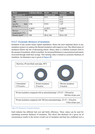
Various charts, graphs and references are available for heat loss computation. The surface heat
loss can be computed with the help of a simple relation as given below. This equation can be
used up to 200°C surface temperature. Factors like wind velocities, conductivity of
insulating material etc has not been considered in the equation.
𝑆 = [10 +
(𝑇𝑠 − 𝑇𝑎)
20
] 𝑋 (𝑇𝑠 − 𝑇𝑎)
Where,
S = surface heat loss in kcal/hr m2
Ts = Hot surface temperature in °C
Ta = Ambient temperature in °C
Total heat loss/hr = S X A
Where,
A is the surface area in m2
Based on the cost of heat energy, the quantification of heat loss in Nu. can be calculated as
follows:
𝐸𝑞𝑢𝑖𝑣𝑎𝑙𝑒𝑛𝑡 𝑓𝑢𝑒𝑙 𝑙𝑜𝑠𝑠, 𝑘𝑔/𝑦𝑒𝑎𝑟 =
Total heat loss per hour X annual hours of operation
𝐺𝐶𝑉 𝑋 𝐵𝑜𝑖𝑙𝑒𝑟 𝑒𝑓𝑓𝑖𝑐𝑖𝑒𝑛𝑐𝑦
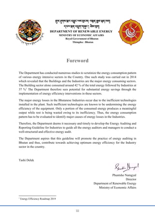
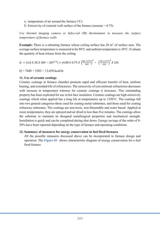
Case Example
Steam pipeline 100 mm diameter is not insulated for 100 metre length supplying steam at 10
kg/cm2
to the equipment. Find out the fuel savings if it is insulated with 65 mm insulating
material.

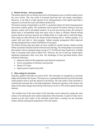
238. 224
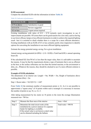
Given:
Boiler efficiency = 80%
Fuel oil cost = Nu. 15,000/t
Surface temperature without insulation, Ts = 170°C
Surface temperature after insulation, = 65°C
Ambient temperature, Ta = 25°C
Solutions:
Calculating Existing heat loss
𝑆 = [10 +
(170 − 25)
20
] 𝑋 (170 − 20) = 2500 kcal/hr − m2
Modified system
After insulating with 65 mm glass wool with aluminium cladding, the expected hot face
temperature will be 65°C
Ts = 65°C
Ta = 25°C
Substituting these values
𝑆 = [10 +
(65 − 25)
20
] 𝑋 (65 − 20) = 480 kcal/hr − m2
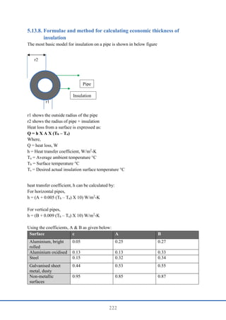
Table 41: Fuel savings calculation
Pipe dimension = 100 mm diameter & 100 m length
Surface area existing = 3.14 X 0.1 X 100 = 31.4 m2
Surface area after insulation = 3.14 X 0.23 X 100 = 72.2 m2
Total heat loss in existing system = 2500 X 31.4 = 78,500 kcal/hr
Total heat loss in modified system = 480 X 72.2 = 34,656 kcal/hr
Reduction in heat loss 78500 – 34656 = 43,844 kcal/hr
No. of hours operation in a year 8400
Total heat loss (kcal/year) 43844 X 8400 = 3,682,89,600
GCV of fuel oil 10,300 kcal/kg
Boiler efficiency 80%
Price of fuel oil Nu. 35000/t
Yearly fuel oil savings = (3,682,89,600 / 10,300) X 0.8
= 44,695 kg/year
Cold insulation
Cold Insulation should be considered and where operating temperature are below ambient
where protection is required against heat gain, condensation or freezing. Condensation will
occur whenever moist air comes into contact with the surface that is at a temperature lower
than the dew point of the vapour. In addition, heat gained by uninsulated chilled water lines
can adversely affect the efficiency of the cooling system.

239. 225
The most important characteristics of a suitable Cold insulation material have following
features:
• Low thermal conductivity
• High water resistance, and
• Durability at low temperature
Other properties like easy workability, negligible capillary absorption should also be taken
into consideration while making a selection. The insulation system is only as good as its
vapour barrier and the care with which it is installed.
Material selection for cold insulation
Selection of insulation materials should be carefully considered where the possibility of steam
purging of the equipment is required or for other reasons which may cause the temperature to
be increased to a level that exceeds the maximum limiting temperature of the insulation
materials, i.e., material then deteriorate. Examples of cold insulation include Urethane Foam,
Expanded Polystyrene, Resin bonded glass wool, Resin Bonded Glass wool, and Phenolic
Foam.
Economics of cold insulation
Unlike hot insulation system, the concern area in Cold Insulation is the heat gain into the
refrigerated space, which leads to increase in the refrigeration load (TR) & energy consumption
as a consequence. The cost of heat gain can thus be assessed & evaluated against cost of
additional cold insulation thickness, to optimize overall energy consumption & cost in
refrigeration system.
Refractories
Any material can be described as 'refractory,' if it can withstand the action of abrasive or
corrosive solids, liquids or gases at high temperatures. For example, fireclay, alumina,
magnesite, chrome magnesite, dolomite etc. Refractory materials are made in varying
combinations and shapes and for different requirements of high temperature processes carried
out in metal extraction, cement, glassmaking, manufacturing, ceramic etc.
The general requirements of a refractory material can be summed up as:
 Ability to withstand high temperatures.
 Ability to withstand sudden changes of temperatures.
 Ability to withstand action of molten metal slag, glass, hot gases, etc.
 Ability to withstand load at service conditions.
 Ability to withstand load and abrasive forces.
 Low coefficient of thermal expansion.
 Should be able to conserve heat.
 Should not contaminate the material with which it comes into contact.

240. 226
Some useful insulating materials to minimise heat losses
Insulating materials greatly reduce the heat losses through walls. Insulation is done by
providing a layer of material having a low heat conductivity between the internal hot surface
of a furnace and the external surface, thus causing the temperature of the external surface
reduced. Insulating materials owe their low conductivity to their pores while their heat capacity
depends on the bulk density and specific heat. Structure of air insulating material consists of
minute pores filled with air which have in themselves very low thermal conductivity, excessive
heat affects all insulation material adversely, but the temperatures to which the various
materials can be heated before this adverse effect occurs differ widely. Clearly, therefore, the
choice of an insulating material must depend upon its effectiveness to resist heat conductivity
and upon the temperature that it will withstand.
Ceramic Fibre
Ceramic fibre is a low thermal mass insulation material, which has revolutionised the furnace
design lining systems. Ceramic fibre is an alumina silicate material manufactured by blending
and melting alumina and silica at temperature of 1800-2000°C and breaking the molten stream
by blowing compressed air or dropping the melt on spinning disc to form loose or bulk ceramic
fibre. The bulk fibre is converted to various products including blanket, strips, veneering and
anchored modules, paper, vacuum formed boards and shapes, rope, wet felt, mastic cement etc.
for insulation applications.
These fibres are generally produced in bulk wool form and needled into blanket mass of various
densities ranging from 64 to 190 kg/m3
Converted products and over 40 different forms are
made from blankets to suit various requirements.
High Emissivity Coatings
Emissivity, the measure of a material's ability to both absorb and radiate heat, has been
considered by engineers as being an inherent physical property which like density, specific
heat and thermal conductivity, is not readily amenable to change. However, the development
of high emissivity coatings now allows the surface emissivity of materials to be increased, with
resultant benefits in heat transfer efficiency and in the service life of heat transfer components.
High emissivity coatings are applied in the interior surface of furnaces. High emissivity coating
shows a constant value over varying process temperatures.
The application of high-emissivity coatings in furnace chambers promotes rapid and efficient
transfer of heat, uniform heating, and extended life of refractories and metallic components
such as radiant tubes and heating elements. For intermittent furnaces or where rapid heating is
required, use of such coatings was found to reduce fuel or power to tune of 25-45%. Other
benefits are temperature uniformity and increased refractory life. Furnaces, which are operate
at high temperatures have emissivity’s of 0.3. By using high emissivity coatings this can go up
to 0.8 thus effectively increasing the radiative heat transfer. The Figure 91 below shows high
emissivity of various insulating materials including high emissivity coatings.

241. 227
Figure 91: High emissivity coatings of various insulating materials
Castable and Concretes
Monolithic linings and furnace sections can be built up by casting refractory insulating
concretes, and by stamping into place certain light weight aggregates suitably bonded. Other
applications include the formation of the bases of tunnel kiln cars used in the ceramic industry.
The ingredients are similar to those used for making piece refractories, except that concretes
contain some kind of cement, either Portland or high-alumina cement.

242. 228
5.14. Renewable energy systems
Scope in energy audit
The inclusion of Renewable energy in energy audits depends upon the focus of the audit and
the objectives of the client organization management team. If the organisational goal is to
reduce the overall carbon footprint, then it will come under renewable energy focused areas.
Whereas if the organisation’s goal is to reduce the energy, this will come under the scope of
energy audit. Also, it should be noted that low-cost or no-cost opportunities should be of prime
focus. Principle which focusses on reducing the size of the renewable system required or to
save the energy wastage should be followed under renewable energy audits.
The solar systems are available in various sizes depending upon the application. Over the years
as the technology has improved the efficiency of these solar energy collector has improved and
there are a lot of varieties available. The amount of electricity generated is dependent on several
factors: the size and arrangement of the system, module type, the available sunlight, and the
efficiency of the electrical components used to covert solar energy into electricity.
Stand-alone PV System
A free standing or Stand-alone PV System is made up of a number of individual photovoltaic
modules (or panels) usually of 12 volts with power outputs of between 50 and 100+ watts each.
These PV modules are then combined into a single array to give the desired power output. A
simple standalone PV system is an automatic solar system that produces electrical power to
charge banks of batteries during the day for use at night when the suns energy is unavailable.
A stand-alone small-scale PV system employs rechargeable batteries to store the electrical
energy supplied by a PV panels or array.
Stand-alone PV systems are ideal for remote rural areas and applications where other power
sources are either impractical or are unavailable to provide power for lighting, appliances, and
other uses. In these cases, it is more cost effective to install a single stand-alone PV system
than pay the costs of having the local electricity company extend their power lines and cables
directly to the home.
A stand-alone photovoltaic (PV) system is an electrical system consisting of and array of one
or more PV modules, conductors, electrical components, and one or more loads. But a small-
scale PV system does not have to be attached to a roof top or building structures for domestic
applications, they can be used for camper vans, RV’s, boats, tents, camping and any other
remote location. Many companies now offer portable solar kits that allow you to provide your
own reliable and free solar electricity anywhere you go even in hard to reach locations.

243. 229
Figure 92: Stand-alone PV system (Source: Apricus solar)
Solar potential in Bhutan
According to International Renewable Energy Agency (IRENA), Bhutan has the potential of
12 GW of solar generation capacity. The solar resource data show that Bhutan has an adequate
resource for flat-plate collectors, with annual average values of global horizontal solar radiation
ranging from 4.0 to 5.5 kWh/m2
per day (4.0 to 5.5 peak sun hours per day). Various other
parameters related to the solar energy are mentioned below.
Direct Normal Solar Radiation: Figure 93 shows the annual average direct normal radiation
which are important for solar thermal system. The DNI varies between 2.5 and 5.0 kWh/m2
per
day. The best DNI resource is in some of the high-altitude areas in the far north of the country.
Average DNI estimate of less than 6.0 or 7.0 kWh/m2
per day is insufficient for concentrating
solar power systems.

244. 230
Figure 93: Direct Normal Irradiation map of Bhutan (Source: World bank group)
Global Horizontal Solar Radiation: Figure 94 shows the annual average GHI, which is
considered for flat plate solar collector applications. The values range from 4.0 to 5.5 kWh/m2
per day. From the figure it is clear that the solar resource for flat-plate collectors is available
for Bhutan. The best resource is in the northern part of the country with a few in the central-
west portion near Paro and just north of Wangdue. In Bhutan's rural electrification program,
estimations of solar home system production use an annual average GHI value of 4.4 kWh/m2
per day (NREL).

245. 231
Figure 94: Global Horizontal Irradiation (Source: World bank group)
Data collection to estimate solar PV potential
If a solar PV is not installed, following data shall be collected from site for solar potential
estimate
 Connected load (kW)
 Actual average load (kW)
 Average monthly electricity consumption (kWh)
 Critical load (needs to ON most of the time)
 Annual working days
 Available area, rooftop or ground in m2
 If available area is rooftop than find type of rooftop (tiles/corrugated metals/others)
Data collection for solar PV audit
If a solar PV is already installed, following data shall be collected during audit:
 Average electricity generation by solar plant per month and year (kWh/month,
kWh/year)
 DC power output from PV module (kW) or DC power input to inverter (kW)
 AC power input from inverter (kW)
 Array area (m2
)
 GPS location of solar plant

246. 232
Instruments required
 Measuring tape or Distance meter
 Hand-held clamp meter
 Compass
Performance terms
 Performance ratio
 Solar PV module efficiency
 Inverter efficiency
 System efficiency
 Capacity utilisation factor
Performance assessment of the PV system
The performance of solar photovoltaic power plant work can be done manually as well as
automatically using various software’s or tools. The tools imports meteorological data from
many different sources and help to predict the performance of the system. Software can
evaluate the performance of grid-connected, stand-alone and pumping systems based on the
specified module selection. The program accurately predicts the system yields computed using
detailed hourly simulation data. Solar GIS is a geographic information system designed to meet
the needs of the solar energy industry. The application combines solar resource data and
meteorological data with a web-based application system to support planning, development,
and operation of solar energy systems.
While in order to evaluate the performance of SPV plant manually, it required to understand
various parameters. These parameters are the indicators of the performance of the plant and
can be used by the auditor for evaluating the plant performance.
Performance Ratio
The performance ratio (PR) indicates the overall effect of losses on a PV array’s normal power
output depending on array temperature and incomplete utilization of incident solar radiation
and system component inefficiencies or failures. Also defined as a ratio of the final yield
divided by the reference yield and it represents the total losses in the PV system when
converting from DC to AC. It indicates how close it approaches ideal performance during real
operation and allows comparison of PV systems independent of location, tilt angle, orientation,
and their nominal rated power capacity. Performance ratio will also consider the availability of
the grid, minimum level of irradiation needed to generate electrical energy.
Performance ratio is defined by the following equations as
𝑃𝑅 (%)
=
𝑇𝑜𝑡𝑎𝑙 𝐴𝐶 𝐸𝑛𝑒𝑟𝑔𝑦 𝑂𝑢𝑡𝑝𝑢𝑡(𝑘𝑊ℎ)
𝐺𝑙𝑜𝑏𝑎𝑙 𝐼𝑟𝑟𝑎𝑑𝑖𝑎𝑡𝑖𝑜𝑛, (𝑘𝑊ℎ/𝑚2) 𝑋 𝐴𝑟𝑟𝑎𝑦 𝑃𝑙𝑎𝑛𝑒 𝐴𝑟𝑒𝑎(𝑚2) 𝑋 𝑃𝑎𝑛𝑒𝑙 𝐸𝑓𝑓𝑖𝑐𝑖𝑒𝑛𝑐𝑦
𝑋 100

247. 233
Solar PV module efficiency
Solar panel efficiency is a measurement of a solar panel’s ability to convert sunlight into usable
electricity. The efficiency is the most used parameter to compare the performance of one solar
cell to another. In addition to reflecting the performance of the solar cell itself, the efficiency
depends on the spectrum and intensity of the incident sunlight and the temperature of the solar
cell. Different types of materials used in manufacturing of solar panel yields possess different
efficiencies. Today, most solar panels have efficiencies between 15% and 20%. The
instantaneous PV module conversion efficiency is calculated in the equation.
𝑃
𝑚𝑎𝑥 = 𝑉𝑂𝐶 𝑋 𝐼𝑆𝐶
Where,
Voc is the open-circuit voltage
Isc is the short-circuit current
𝜂𝑃𝑉 =
𝐷𝐶 𝑝𝑜𝑤𝑒𝑟 𝑜𝑢𝑡𝑝𝑢𝑡 𝑓𝑟𝑜𝑚 𝑡ℎ𝑒 𝑃𝑉 𝑚𝑜𝑑𝑢𝑙𝑒 (𝑘𝑊)
𝐺𝑙𝑜𝑏𝑎𝑙 𝐼𝑟𝑟𝑎𝑑𝑖𝑎𝑡𝑖𝑜𝑛 𝑘𝑊/𝑚2 𝑋 𝐴𝑟𝑟𝑎𝑦 𝑎𝑟𝑒𝑎(𝑚2)
𝑋 100
Inverter efficiency
It is the comparison of the amount of the total AC power obtained after the inverter with the
DC power generated by the solar panel. In order to maintain a good overall system efficiency,
it is required that an appropriate inverter is selected for the system. The instantaneous PV
module conversion efficiency is calculated in the equation.
𝜂𝑖𝑛𝑣 =
𝐴𝐶 𝑝𝑜𝑤𝑒𝑟 𝑜𝑢𝑡𝑝𝑢𝑡 𝑓𝑟𝑜𝑚 𝑡ℎ𝑒 𝑖𝑛𝑣𝑒𝑟𝑡𝑒𝑟 (𝑘𝑊)
𝐷𝐶 𝑝𝑜𝑤𝑒𝑟 𝑖𝑛𝑝𝑢𝑡 𝑡𝑜 𝑡ℎ𝑒 𝑖𝑛𝑣𝑒𝑟𝑡𝑒𝑟 (𝑘𝑊)
𝑋 100
System efficiency
System efficiency is a collective term that include efficiencies of various electrical equipment
present in the system along with various other efficiencies that affects the system. The
instantaneous PV module conversion efficiency is calculated in the equation.
𝜂𝑃𝑉 =
𝐴𝐶 𝑝𝑜𝑤𝑒𝑟 𝑜𝑢𝑡𝑝𝑢𝑡 𝑓𝑟𝑜𝑚 𝑡ℎ𝑒 𝑠𝑦𝑠𝑡𝑒𝑚 (𝑘𝑊)
𝐺𝑙𝑜𝑏𝑎𝑙 𝐼𝑟𝑟𝑎𝑑𝑖𝑎𝑡𝑖𝑜𝑛 𝑘𝑊/𝑚2 𝑋 𝐴𝑟𝑟𝑎𝑦 𝑎𝑟𝑒𝑎(𝑚2)
𝑋 100
Capacity Utilisation Factor (CUF)
It is the ratio of the actual output from a solar plant over the year to the maximum possible
output from it for a year under ideal conditions. If the system delivers full rated power
continuously, its CF would be unity. It is dependent on the location, orientation, tilt angle
unlike the Performance ratio.
𝐶𝑈𝐹(%) =
𝐸𝑛𝑒𝑟𝑔𝑦 𝑜𝑢𝑡𝑝𝑢𝑡 (𝑘𝑊ℎ)
𝑇𝑜𝑡𝑎𝑙 𝐼𝑛𝑠𝑡𝑎𝑙𝑙𝑒𝑑 𝐶𝑎𝑝𝑎𝑐𝑖𝑡𝑦 (𝑘𝑊) 𝑋 𝑡𝑖𝑚𝑒 𝑝𝑒𝑟𝑖𝑜𝑑 (ℎ𝑟𝑠)
𝑋 100

248. 234
Specific plant losses
Energy losses occur in various components in a SPV Power plant under real operating
conditions. These losses are evaluated using the monitored data.
There exist a variety of sources through which energy losses occur in PV systems. These losses
affect the performance of PV systems thereby justifying why, it is necessary to evaluate these
losses using detailed performance monitoring data. Prominent among these losses are array
capture losses, shading losses, system losses, cell temperature losses, soiling and degradation.
Soiling and degradation losses are more difficult to evaluate because they are small effects that
occur over large fluctuations in operating conditions.
The International Electrotechnical Commission (IEC) prepares and publishes international
standards for photovoltaic systems that convert solar energy into electrical energy, as well as
for all the elements in the entire photovoltaic energy system. In case of detail specific or
performance monitoring these testing, procedures needs to be followed. The standards are used
for testing and monitoring the module performance. Some of them are mentioned below:
IEC 60891 Photovoltaic devices - Procedures for temperature and irradiance corrections to
measured I-V characteristics
IEC 61853-2: Scope of work in progress includes spectral response, incidence angle and
module operating temperature measurements for PV module performance testing and energy
rating.
IEC 61683 Power conditioners – Procedure for measuring efficiency
Effect of temperature on solar efficiency
The power generation from the PV plant is greatly affected by the temperature. If the
temperature of the module goes beyond the rated module temperature, the power generated is
much less when compared to the power generated when the temperature equals or is marginally
greater than the rated temperature. This effect appears on the output voltage of the cell, where
the voltage is indirectly proportional to the temperature, i.e. the decrease in voltage is caused
by an increase in the cell temperature.

249. 235
Figure 95: Effect of temperature change on power and voltage
Solar PV facts
 The area required to install 1 kWp capacity solar PV system is approx. 8 to 10 m2
.
 Solar panels produce approx. 10 kWh of electricity per square foot.
 It is possible to install a solar PV system without battery to reduce installation cost.
 The orientation of solar panels (solar angles) are best aligned according to the latitude
of location.
 Solar PV also produces electricity during cloudy days, but in lesser amount.
 Most solar panels come with a 25-year warranty. Solar energy is a completely free
source of energy and is found in abundance. Solar energy can also be used to generate
hot water or steam for process applications in industries.

250. 236
Solar water heating system
Solar water heating system is a device that uses solar energy to heat water for domestic,
commercial, and industrial needs. Water is heated during the daytime and is stored in a tank
which makes it available throughout the day as well night due to insulation provided over the
tank. The system is generally installed on the roof or open ground, with the collector facing the
sun and connected to a continuous water supply. The sun rays have heats up the water up to
55°C to 70°C which is more than enough for various applications. The water remains at
required temperature for a duration of approximately two days.
For use in cloudy days, as a backup the system is consist of an electrical heating system. The
estimated life of a solar water heater is 15 to 20 years. A typical solar water heating system
roughly can save up to 1500 units of electricity every year, for every 100 litres per day of solar
water heating capacity.
Figure 96: Solar water heater
Data collection to estimate solar water heating potential
If a solar thermal system is not installed, following data shall be collected to estimate solar
water heating potential:
 Amount of hot water required per day (kl/day)
 Available roof top or ground area (m2
)
 Existing system of water heating
 Existing energy usage for water heating
 Type of process and other relevant details

251. 237
Selection of a solar water system
The following factors are considered while selecting an appropriate solar water heating system
for any facility.
1. Types of panels
There are basically two types of solar panel commonly available are:
Flat plate collector
Flat plate solar panels are commonly used collectors that has a metal plate with a dark-coloured
coating to absorb heat. Pipes under the plate contain water or some other fluid such as glycol,
which absorbs heat and carries it to the water in the storage cylinder. A transparent cover,
usually glass, admits solar radiation but stops it from escaping. The construction is simple, with
no moving parts, which means they are easily repaired. They are relatively low cost and can
supply water at temperatures up to 95ºC, though efficiency diminishes rapidly above 70ºC, so
systems should be sized to avoid these sorts of temperatures.
Evacuated glass tube collector
Evacuated glass tube solar panels are made up of several glass tubes, typically 20 or more.
Each tube has a vacuum to reduce convection and conduction heat losses. Evacuated tubes may
contain an absorber plate connected to pipes through which a heat-absorbing fluid circulates or
a heat pipe that contains an evaporating/condensing fluid to transfer heat.
Individual tubes sometimes fail but can be replaced at relatively low cost.
2. Sizing the panels
The size of the panel depends on the water storage capacity available and is typically based on
a ratio of about 1 square meter of panel for each 50–70 litres of cylinder volume. Most panels
commercially available are in the 3–8 m² range.
3. Positioning to maximize solar heat absorption
The heating capacity of a solar water heating system is directly proportional to the amount of
solar radiation absorbed, which depends on the following factors:
 Solar intensity: That is the available solar radiation energy (kWh/m²) at a location.
 Solar panel area: The larger the area, the more heat can be produced.
 Solar panel tilt angle: The optimum installed angle for solar absorption is
perpendicular to the sun. But due to the continuous change in sun’s position an
optimal angle is chosen to maximize the utilization.
 Solar panel orientation: The positioning of the panel to maximize the solar energy
considering the suns movement.
Efficiency of collector
The efficiency and effectiveness of a solar water heating system depends on the size, type of
panels used, and on positioning them to maximize absorption of solar radiation. Although for
basic evaluation of performance of solar water heater, the efficiency of the system needs to be
monitored. Collector efficiency can be given as the ratio between the solar energy incident on
the panel to the available thermal energy at the application site.

252. 238
Efficiency can be shown in the equation as follows:
𝜂 =
𝐻𝑒𝑎𝑡 𝑒𝑛𝑒𝑟𝑔𝑦 𝑎𝑣𝑎𝑖𝑙𝑎𝑏𝑙𝑒
𝐼𝑛𝑐𝑖𝑑𝑒𝑛𝑡 𝑆𝑜𝑙𝑎𝑟 𝑒𝑛𝑒𝑟𝑔𝑦
=
𝑄𝑜𝑢𝑡
𝑄𝑖𝑛
Where,
𝑄𝑖𝑛 = 𝐴𝑐 𝑋 𝐺𝑡
𝑄𝑜𝑢𝑡 = 𝑚 𝑋 𝐶𝑝 𝑋 (𝑇𝑜𝑢𝑡 − 𝑇𝑖𝑛)
𝜂 =
𝑚 𝑋 𝐶𝑝 𝑋 𝐹𝑅 𝑋 (𝑇𝑜𝑢𝑡 − 𝑇𝑎)
𝐴𝑐 𝑋 𝐺𝑡
Where,
Qout = the energy absorbed by the collector (W/m2
)
m = mass of water going into the collector (kg/s)
Cp = specific heat capacity of water
AC = the size of the collector (m2
)
FR = collector heat loss factor
Gt = total solar radiation intensity (W/m2
)
Tin = temperature of incoming water
Tout = temperature of the outgoing water
Ta = ambient temperature

253. 239
Raw material
Chemical
Water
Reusable waste
Products
Recycle
By-products
Wastewater
Solid waste
Liquid waste
Gaseous emissions
6 Analysis of Energy Use and Material Balance
6.1. Introduction
A material balance in its most broad definition is the application of the law of conservation of
mass, which states matter is neither created nor destroyed. Matter may flow through a control
volume and may be reacted to form another species, however, no matter is ever lost or gained.
The same is true for energy. As with material balances, we can apply the law that energy is
neither created nor destroyed, it is simply converted into another form of energy. The law of
conservation of mass and energy leads to what is called a mass (material) and energy balance.
Material balances, as they pass through processing operations, can describe material quantities.
If there is no accumulation, what goes into a process must come out. This is true for batch
operation. It is equally true for continuous operation over any chosen time interval.
Material balances are fundamental to the control of processing, particularly in the control of
yields of the products. Material balance can be determined from conceptual stage to final
production stage. Initially, material balance is estimated during the planning stage of a new
process or equipment. This estimate is improved while carrying out pilot scale tests related to
the new process. This material balance is verified during commissioning stage and finally used
as a control measure during actual production stage.
Energy balances are means for industry to examine ways of reducing energy consumption in
processing because of increasing energy cost. Energy balances are used in the examination of
the various stages of a process, over the whole process and even extending over total production
system from the raw material to the finished product.
6.2. Purpose of energy and material balance
 To assess the input, conversion efficiency, output and losses
 To quantify all material, energy and waste streams in a process or a system
 Powerful tool for establishing basis for improvement and potential savings
6.3. Component of energy and material balance
Typical components of material and energy balance for a process or unit operation is shown in
below figure It may be noted that recycle stream is shown along with input side.
Process or Unit Operations
Energy

254. 240
6.4. Basic principles of energy and material balance
If the industry operation, whatever its nature is seen as a whole it may be represented
diagrammatically as a box as shown in Figure 97 The mass and energy going into the box must
balance with the mass and energy coming out.
The law of conservation of mass leads to what is called a mass or material balance.
Mass in = Mass Out + Mass stored
∑Raw materials = ∑Products + ∑Wastes + ∑Stored materials
m = p + w + s
If there are no chemical changes occurring in the plant, the law of conservation of mass will
apply also to each component. For example, in a plant that is producing sugar, if the total
quantity of sugar (m) going into the plant is not equalled by the total of the purified sugar (p)
and the sugar in the waste liquors (w) and accumulated in the process (s), then there is
something wrong. Sugar is either being burned (chemically changed) or else it is going
unnoticed down the drain somewhere. In this case:
m = p + w + s + l
where, l is the unknown loss and needs to be identified so, the material balance is now:
Raw materials = Products + waste products + stored products + Losses
Where, losses are the unidentified materials.
Just as mass is conserved, energy is conserved in process operations. The energy coming into
a unit operation can be balanced with the energy coming out and the energy stored.
∑Energy in = ∑Energy out + ∑Energy stored
∑Em = ∑Ep + ∑Ew +∑Es + ∑El
Where,
∑Em = Total energy entering with raw materials
∑Ep = Total energy leaving with products
∑Ew = Total energy leaving with waste materials
∑Es = Total energy stored
∑El = Total energy lost to surroundings

255. 241
Figure 97: Energy and material balance representation
Energy balances are often complicated because forms of energy can be inter-converted, for
example mechanical energy to heat energy, but overall, the quantities must balance.
6.5. Classification of process
Process can be viewed overall or as a series of units. Each unit is a unit operation that can be
represented by a box as shown in Figure 98 Raw materials and energy go into the box and
desired products, by-products, wastes and energy come out of the box. The mass in and out of
a control box must be equal. The equipment within the box will make the required changes
with little waste and energy as possible. There are different types of process.
Products, p
Unit operation
Stored material, s
Stored energy, Es
Waste, w
Raw
material, m
Energy, Em
Energy, Ep
Energy, Ew
Energy, El

256. 242
Figure 98: Classification of process
A) Based on how the process varies with time
Steady-state process is one where none of the process variables change with time Unsteady-
state process is one where the process variables change with time
B) Based on how the process was built to operate
A continuous process is one that has the feed streams and product streams moving into and out
of the process all the time. Examples are oil refinery, distillation process etc.
A batch process is one where the feed streams are fed to the process to get it started. The feed
material is then processed through various process steps and finished products are taken out at
specific times.
Steps:
 Feed is charged into vessel
 Process is started
 No mass is added or removed from vessel (process parameters are usually monitored
and controlled)
 At some conditions or after fixed time, products are removed
Material Balance
Levels of Material Balance
The material balances can be developed at various levels:
Wasted energy
Control
Energy
Unit Operations
Previous Unit
operations
Subsequent Unit
operations
By-products & waste

257. 243
Overall Material balance: This involves input and output steams for complete plant
Section wise Material balances: This involves M&E balances to be made for each
section/department/cost centre. This would help to prioritise focus areas for efficiency
improvement
Equipment-wise Material balances: Material balances for key equipment would help assess
performance of equipment, which would in turn help identify energy and material losses.
The choice among the types of material balance depends on the reasons for making the
balance. The major factor is the cost of the materials and so costly materials are more likely
consider than cheaper ones and products more than waste materials
Material balance procedure
First step is to identify materials in, materials out and material stored. Next step is to consider
whether materials in each category have to be treated as whole (gross material balance) or
whether individual constituents in the material should be treated separately. For example, we
can do material balance for dry solids alone as opposed to total material. This means
separating the material into two constituents’ non-water and water.
Typical steps are as follows:
a) Define basis & units: Choose a basis of calculations on quantity (mass for batch process)
or flow rate (mass per hour for continuous process) of one of the process streams. Convenient
Units are then chosen as mass can be expressed in various ways: weight/weight
(wlw)weight/volume (wlv)molar concentration (M), mole fraction.
 The weight/weight concentration is the weight of the solute divided by the total
weight of the solution and is the fractional form of the percentage composition by
weight.
 The weight volume concentration is the weight of solute in the total volume of the
solution with gases concentrations are primarily measured in weight concentrations
per unit volume, or as partial pressures.
 The molar concentration is the number of molecular weights of the solute expressed
in kg in 1 m3
of the solution.
 The mole fraction is the ratio of the number of moles of the solute to the total number
of moles of all species present in the solution.
b) Draw a flow chart: Establish a boundary so that the flow streams in and out can be
identified. The identification and drawing up a unit operation/process is prerequisite for
energy and material balance. Flow charts are schematic representation of the production
process involving various input resources conversion steps and output and recycle streams.
The process flow may be constructed stepwise i.e. by identifying the inputs Ioutput I wastes
at each stage of the process, as shown in the refer Figure 2 of Chapter 4.1

258. 244
Inputs of the process could include raw materials, water, steam, energy (electricity, etc.)
Process Steps should be sequentially drawn from raw material to finished product.
Intermediates and any other by-product should also be represented. The operating process
parameters such as temperature, pressure, % concentration, etc. should be represented.
The flow rate of various streams should also be represented in appropriate units like m3
/h or
kg/h. In case of batch process, the total cycle-time should be included.
Wastes by-products could include solids, water, chemicals, energy etc. For each process steps
(unit operation) as well as for an entire plant, energy and mass balance diagram should be
drawn. Output of the process is the final product produced in the plan
c) Write material balance equations: The following examples are illustration for writing
the material balance equations
Example: Skim milk is prepared by the removal of some of the fat from whole milk. This skim
milk is found to contain 90.5% water, 3.5% protein, 5.1% carbohydrate, 0.1% fat and 0.8%
ash. If the original milk contained 4.5% fat, calculate its composition assuming that fat only
was removed to make the skim milk and that there are no losses in processing.
Basis:100 kg of skim milk.
This contains, therefore, 0.1 kg of fat. Let the fat which was removed from it to make skim
milk be 𝑥 kg.
Total original fat = (𝑥 +0.1) kg
Total original mass= (100 + 𝑥) kg
and as it is known that the original fat content was 4.5% so
(𝑥 + 0.1)
(100 + 𝑥)
= 0.45
𝑥 + 0.1 = 0.45 (100 + 𝑥)
𝑥 = 4.6 𝑘𝑔
Let fat = 𝑥
Original milk / whole
milk, 4.5%
90.5% water, 3.5% protein,
5.1% carbohydrate, 0.1% fat
and 0.8%ash

259. 245
So, the composition of the whole milk is then fat = 4.5%, water = 90.5/104.6 = 86.5 %,
protein = 3.5/104.6 = 3.3 %, carbohydrate= 5.1/104.6 = 4.9% and ash= 0.8%
Example: A bag filter is used to remove the dust from the inlet gas stream to meet the emission
standards in cement, fertilizer and other chemical industries.
Inlet gas to a bag filter is 1,69,920 m3
/hr and the dust loading is 4577 mg/m3
Outlet gas from the bag filter is 1,85,040 m3
/hr and the dust loading is 57 mg/m3
What is the maximum quantity of ash that will have to be removed per hour from the bag filter
hopper based on test results?
Solution:
Dust balance, mass in = mass out
Inlet gas duct = outlet gas duct + hopper ash
Inlet dust quantity = 1,69,920 (m3
/hr) X 4,577 (mg/m3
) X (1/10,00,000) kg/mg =
777.7 kg/hr
Outlet dust quantity = 1,85,040 (m3
/hr) X 57 (mg/m3
) X (1/10,00,000) kg/mg
= 10.6 kg/hr
Hopper ash = Inlet quantity – Outlet dust quantity
= 777.7 kg/hr – 10.6kg/hr
= 767.1 kg/hr
Original milk / whole
milk, 4.5%
90.5% water, 3.5% protein,
5.1% carbohydrate, 0.1% fat
and 0.8%ash
𝑥 = 4.6 𝑘𝑔
104.6 kg
100 kg

260. 246
6.6. Energy balance
Energy is the capacity to do work or to transfer heat. The law of conservation of energy
states that energy can neither be created nor destroyed. The total energy in the materials
entering the processing plant, plus the energy added in the plant must equal the total energy
leaving the plant. This is a more complex concept than the conservation of mass, as energy can
take various forms such as kinetic energy, Potential energy, heat energy, chemical energy,
electrical energy and so on. During processing, some of these forms of energy can be converted
from one to another; say for instance mechanical energy in a fluid can be converted through
friction into heat energy. It is the sum total of all these forms of energy that is conserved.
For example, in the pasteurizing process for milk, the milk is pumped through a heat exchanger
and is first heated and then cooled. The energy affecting the product is the heat energy in the
milk. Heat energy is added to the milk by the pump and by the hot water passing through the
heat exchanger. Cooling water then removes part of the heat energy and some of the heat energy
is also lost to the surroundings. The heat energy leaving in the milk must equal the heat energy
in the milk entering the pasteurizer plus or minus any heat added or taken away in the plant.
Heat energy leaving in milk = initial heat energy + heat energy added by pump + heat
energy added in heating section - heat energy taken out in cooling section - heat energy lost
to surroundings.
The law of conservation of energy can also apply to part of a process. For example,
considering only the heating section of the heat exchanger in the pasteurizer, the heat lost by
the hot water must be equal to the sum of the heat gained by the milk and the heat lost from
the heat exchanger to its surroundings.
Conservation of energy
In a system, if the storage does not change, the ingoing and outgoing energy must be
equal Figure 99 a
If the storage changes, this must be reflected in the energy balance and the energy input to
a system might not balance the energy that goes out. For instance, as in Figure 99 b, the
input is 75 units of energy but only 60 units go out. Since the first law requires that the
energy be conserved, system had to gain 15 units of energy. In the Figure 99 c the input is
short by 15 units of energy so it can be inferred that the system must have lost 15 units.

261. 247
Figure 99: Conservation of energy
The sinks are depositories of leakage or rejected energy. It is usually low-grade heat, as in,
radiation losses from boilers or heat carried away by cooling water. The outputs represent
useful work.
Efficiency
The (thermodynamic) efficiency of a process is the ratio of useful output to input and is
always less than 100%. In the energy balance shown in Figure 100, there is no internal
storage, so the sum of the inputs must equal the outgoing energy. The efficiency of the
process is 22.5% and the energy lost in the system is 100 - 22.5 = 77.5%.
Figure 100: Efficiency and losses
Energy analysis and Sankey diagram
The basic data needed for an energy analysis is an energy balance of each process section. The
objective is to define in detail the energy input, energy utilized, and the energy dissipated or
wasted. This is best represented by a Sankey diagram.
The Sankey diagram is very useful tool to represent an entire input and output energy flow
in any energy equipment or system such as boiler generation, fired heaters, furnaces after
carrying out energy balance calculation. Usually the flows are represented by arrows. The
width of the arrows is proportional to the size of the actual flow. Better than numbers, tables
or descriptions, this diagram represents visually various outputs (benefits) and losses so that
25
65
75
45
15
75
15
75
60
Qo
Qo+15 Qo-15
a) No Storage
b) Storage
increased
c) Storage
decreased
155
45
15
185
Qo
Input = 15 + 185
Output + Sink = 45 + 155
Efficiency = Output/Input
η = 45 / (15+185) = .225 or 22.5%

262. 248
energy managers can focus on finding improvements in a prioritized manner. For example,
the Figure 101 shows a Sankey diagram for Boiler fuel input to heat output.
Figure 101: Sankey diagram for Boiler fuel input to heat output

263. 249
7 Benchmarking
Benchmarking can be a useful tool for understanding energy consumption patterns in an
industrial sector and for taking measures to improve energy efficiency. Energy benchmarking
for industry is a process in which the energy performance of an individual plant or an entire
sector of similar plants is compared against a common metric that represents 'standard' or
'optimal' performance. It may also entail comparing the energy performance of a number of
plants against each other.
Since benchmark tool is used for comparison across a number of plants or sectors, there are
two important features they should have. First, because they are applied to plants or sectors of
different sizes and outputs, the metric used should be common irrespective of plant size. The
most common metric used therefore is energy intensity which measures 'energy use per unit of
output'. Second, the tool should be used in a wide range of facilities so as to compensate for
differences in production at similar facilities.
7.1. Industrial benchmarking programs
Benchmarking energy performance of a facility enables energy auditors and managers to
identify best practices that can be replicated. It establishes reference points for managers for
measuring and rewarding good performance. It identifies high-performing facilities for
recognition and prioritizes poor performing facilities for immediate improvement
There are three approaches for energy benchmarking.
1. The first approach is to evaluate an entire industrial sector, such as steel, ferro and
alloy, cement, etc. This evaluation is used to answer the following questions:
 How well is this sector performing compared to how it would perform using the
best available technologies?
 Has the sector been improving over time?
2. The second approach is the comparison of individual plants within a sector. A
benchmark-type indicator is calculated for all the facilities within a sector so that they
can be compared on even terms. This evaluation can answer the following questions:
What is the state- of-the-art performance in this given sector? How does my plant
compare against the state-of-the-art? How does it compare against the majority of
other plants in the sector? In developing benchmarks at the level of individual plants
the issue of proprietary data becomes important. Individual companies are very
reluctant to disclose information about their production processes, particularly if it will
be released to their competitors. It is important that the indicators developed are general
enough not to reveal any proprietary information and that a credible system is
established that encourages plants to trust the process.
3. The third approach for energy benchmarking that has been seen widely in recent years
is for large industries to set themselves energy efficiency goals by using historical best
performance as benchmark. Industries use this approach to set targets for reducing
energy use by certain percentages over given time frames. Companies do not need to
reveal any proprietary information, since the benchmarking is done internally.

264. 250
The key steps in benchmarking include:
1. Determine the level of benchmarking (for example, at equipment level, process line
level, or industry level). In simple terms, setting up the boundary for benchmarking.
2. Develop metrics: select units of measurements that effectively and appropriately
express energy performance of the plant (e.g. kWh/t product, MTOE/ton product, kg/t
product, etc.)
3. Conduct comparisons to determine the performance of the plant or system being studied
compare to the benchmark.
4. Track performance over time to determine if energy performance being improved or
worsening over time in order to take the appropriate actions
While conducting benchmarking, the key drivers of energy use should be identified and the
benchmarking metrics might be adjusted or normalized, for instance, based on the weather,
production levels, or product characteristics that affect energy use. Normalizing data ensures a
meaningful comparison and avoids comparing “apples to oranges.” Evaluating and acting on
benchmarking results are as important as undertaking the benchmarking activity. Below are
some examples of benchmarking parameters for various industries:
Table 42: Benchmarking parameters for various industries
Industry Benchmarking
parameter or
specific energy
consumption (SEC)
Process parameters need to be
stated for meaningful
comparison among similar
industries
Cement Industry kWh/t of cement
produced
type of cement, blaine number
(cement fineness) i.e. Portland and
process used (wet/dry) are to be
reported alongside kWh/t or in
terms of tons of oil equivalent toe/t
Foundry kWh/t of molten
metal output
Furnace type, composition (mild
steel, high carbon steel/cast iron
etc.) raw material mix, number of
power trips could be some useful
operating parameters to be
reported while mentioning specific
energy consumption data.
Beverages kWh/l of beverage
produced
type of beverage, type of
technology used
Food and agro
products
kWh/kg of food and
agro product
type of product, type of technology
It is evident from above Table 42 that it is not feasible to define a single norms/standard unless
there is significant homogeneity amongst units in a sector. Therefore, it is preferable to fix the
energy efficiency improvements targets as “unit specific” (approach 3).
As per the BEE studies, the wide bandwidth of specific energy consumption (SEC) within an
industrial sector is indicative of the large energy-savings potential in the sector. The wide

265. 251
bandwidth is also a reflection of the differences in the energy-saving possibilities amongst
plants because of their varying technologies deployed, vintage, production capacity, raw
material quality, and product-mix. Such wide variation also makes it difficult to specify a single
benchmark SEC for the sector as a whole: older plants will find the benchmark impossibly high
if it is set at the level of newer plants; newer plants will find it trivial if it is set at the level of
older plants. The broad bandwidth of SEC within a sector, and the inability of all plants to
achieve a sectoral benchmark SEC, suggests that SEC improvement norms need to be set for
individual plants.
7.2. Plant Energy Performance (PEP)
Industry energy performance is the measure of whether a plant is using more or less energy to
manufacture its products than it did in the past, a measure of how well the energy management
program is doing.
Plant energy performance monitoring compares Plant energy use of a reference year and the
subsequent years considering product output to determine the improvement (or deterioration)
that has been made.
However, since the Plant production output varies from year to year it has significant impact
on Plant’s energy use. For a meaningful comparison it is necessary to determine the energy
that would have been required to produce current year’s production output had the plant
operated in the same way as it did during the reference year. This calculated value can then be
compared with the actual value to determine the improvement or deterioration that has taken
place since the reference year.
7.3. Production factor
Production factor is the ratio of production in the current year to that in the reference year.
𝑃𝑟𝑜𝑑𝑢𝑐𝑡𝑖𝑜𝑛 𝑓𝑎𝑐𝑡𝑜𝑟 =
𝐶𝑢𝑟𝑟𝑒𝑛𝑡 𝑦𝑒𝑎𝑟′
𝑠 𝑝𝑟𝑜𝑑𝑢𝑐𝑡𝑖𝑜𝑛
𝑅𝑒𝑓𝑒𝑟𝑒𝑛𝑐𝑒 𝑦𝑒𝑎𝑟′𝑠 𝑝𝑟𝑜𝑑𝑢𝑐𝑡𝑖𝑜𝑛
Production factor is used to determine the energy that would have been required to produce
this year's production output if the plant had operated in the same way as it did in the reference
year.
Reference Year Equivalent Energy Use
The reference years equivalent energy use (or reference year equivalent) is the energy that
would have been used to produce the current year's production output.
The reference year equivalent is obtained by multiplying the reference year energy use by the
production factor (obtained above)
Reference year equivalent = Reference year energy use x Production factor
Plant Energy Performance is the improvement or deterioration from the reference year. It is a
measure of Plant energy progress.

266. 252
𝑃𝑙𝑎𝑛𝑡 𝑒𝑛𝑒𝑟𝑔𝑦 𝑝𝑒𝑟𝑓𝑜𝑟𝑚𝑎𝑛𝑐𝑒
=
𝑅𝑒𝑓𝑒𝑟𝑒𝑛𝑐𝑒 𝑦𝑒𝑎𝑟 𝑒𝑞𝑢𝑖𝑣𝑎𝑙𝑒𝑛𝑡 − 𝐶𝑢𝑟𝑟𝑒𝑛𝑡 𝑦𝑒𝑎𝑟′
𝑠 𝑒𝑛𝑒𝑟𝑔𝑦 𝑢𝑠𝑒
𝑅𝑒𝑓𝑒𝑟𝑒𝑛𝑐𝑒 𝑦𝑒𝑎𝑟 𝑒𝑞𝑢𝑖𝑣𝑎𝑙𝑒𝑛𝑡
𝑋 100
The energy performance is the measure of energy saved at the current rate of use compared to
the reference year rate of use. The greater the improvement; the higher the number will be.
Plant energy performance is the starting point for evaluating energy performance. It does not
require detailed calculations of the energy used by every piece of equipment, or the energy use
of every process. It utilizes the most effective measure of energy savings, the actual
measurement of energy consumption compared to production output. Yearly comparisons
minimize seasonal effects. Once a plant has started measuring yearly energy performance,
management wants more frequent performance information in order to monitor and control
energy use on an on-going basis. In such cases Plant energy performance can just as easily be
used for monthly reporting as yearly reporting.

267. 253
8 Cost Benefit Analysis
After identifying the list of energy-efficiency measures applicable to the facility, the auditor
shall also conduct cost benefit analysis for the measures and make recommendations for their
implementation. Step-by-step guidance for energy auditors on payback period, return of
investment, net present value, and internal rate of return, in order to conduct the common
economic analysis for the assessment of financial viability of the energy efficiency measures
is presented below.
8.1. Payback period
Payback period refers to the amount of time (number of years) it takes to recover the capital
cost of an investment. Shorter payback period means more attractive investments while longer
paybacks are less desirable. It is a simple term to determine whether to go through with an
investment or not.
Simply put, the payback period is the cost of the investment divided by the annual cash
flow or annual net savings and can be calculated using the following equation:
𝑆𝑖𝑚𝑝𝑙𝑒 𝑝𝑎𝑦𝑏𝑎𝑐𝑘 𝑝𝑒𝑟𝑖𝑜𝑑 =
𝐶𝑎𝑝𝑖𝑡𝑎𝑙 𝑐𝑜𝑠𝑡
𝐴𝑛𝑛𝑢𝑎𝑙 𝑛𝑒𝑡 𝑠𝑎𝑣𝑖𝑛𝑔𝑠
Annual net savings is the cost savings achieved after all the operational costs have been met.
The word ‘Simple’ is used as a prefix to the term ‘payback period’ to denote that time value of
money is not considered in its calculation.
Example: A new waste heat recovery system (WHR) installed in a facility is expected to
reduced energy bill by Nu. 400,000. If the capital cost of investment of the new WHR is Nu.
500,000. What will be the expected payback period for the project?
𝑆𝑖𝑚𝑝𝑙𝑒 𝑝𝑎𝑦𝑏𝑎𝑐𝑘 𝑝𝑒𝑟𝑖𝑜𝑑 =
500,000
400,000
= 1.25 𝑦𝑒𝑎𝑟𝑠, 𝑜𝑟 15 𝑚𝑜𝑛𝑡ℎ𝑠
8.2. Return on Investment (ROI)
Return on Investment (ROI) is a performance measure used to evaluate the efficiency of an
investment or compare the efficiency of a number of different investments. ROI tries to directly
measure the amount of return on a particular investment, relative to the investment’s cost. To
calculate ROI, the benefit (or return) of an investment is divided by the cost of the investment.
The result is expressed as a percentage or a ratio.
𝑅𝑂𝐼 =
𝐴𝑛𝑛𝑢𝑎𝑙 𝑛𝑒𝑡 𝑐𝑎𝑠ℎ 𝑓𝑙𝑜𝑤
𝐶𝑎𝑝𝑖𝑡𝑎𝑙 𝑐𝑜𝑠𝑡
𝑋 100

268. 254
Example: An investment of Nu. 100,000 for equipment is expected to provide an after-tax
cash flow of Nu. 25,000 over a period of six years, without significant annual fluctuations.
What is the return of investment?
𝑅𝑂𝐼 =
25,000
100,000
𝑋 100 = 25%
8.3. Net Present Value (NPV)
Net present value (NPV) is the difference between the present value of cash inflows and the
present value of cash outflows over a period of time. NPV is used in capital budgeting and
investment planning to analyse the profitability of a projected investment or project.
The net present value method considers the time value of money. This is done by equating
future cash flow to its current value today, or in other words by determining the present value
of any future cash flow. The present value is determined by using an assumed interest rate,
usually referred to as a discount rate. Discounting is the opposite process to compounding.
Compounding determines the future value of present cash flows, whereas discounting
determines the present value of future cash flows.
The net present value method calculates the present value of all the yearly cash flows (i.e.
capital costs and net savings) incurred or accrued throughout the life of a project and summates
them. As a matter of convention, costs are represented as negative values and savings as
positive values. The sum of all the present values is known as the net present value (NPV). The
higher the net present value, the more attractive is the proposed project.
The following formula is used to calculate NPV:
𝑁𝑃𝑉 = −
𝐶𝐹0
(1 + 𝑖)0
+
𝐶𝐹1
(1 + 𝑖)1
+ … … … +
𝐶𝐹
𝑛
(1 + 𝑖)𝑛
= ∑
𝐶𝐹𝑡
(1 + 𝑖)𝑡
𝑛
𝑡=0
Where,
CFt = Cash flow occurring at the end of year ‘t’ (t =0,1…n) (As per our convention, net
savings or inflows are represented by (+) sign and net costs or outflow are represented by
(-) sign. Since capital investment is an outflow, it will be treated as negative (-) as per our
convention)
i = Discount rate
n = Life of the project
The discount rate (i) employed for evaluating the present value of the expected future cash
flows should reflect the risk of the project. Hence the decision rule associated with the net
present value criterion is: "Accept the project if the net present values is positive and reject the
project if the net present value is negative". A negative net present value indicates that the

269. 255
project is not achieving the return standard and thus will cause an economic loss if
implemented. A zero NPV is value neutral.
The net present value takes into account the time value of money and it considers the cash flow
stream in entire project life.
Example: Using the net present value analysis technique, evaluate the financial merits of the
two proposed projects shown in the table. The annual discount rate is 8% for each of the project.
Projects Project 1 Project2
Capital Cost
(Nu.)
30,000 30,000
Year Net annual
savings (Nu.)
Net annual
savings (Nu.)
1 +6,000 +6,600
2 +6,000 +6,600
3 +6,000 +6,300
4 +6,000 +6,300
5 +6,000 +6,000
6 +6,000 +6,000
7 +6,000 +5,700
8 +6,000 +5,700
9 +6,000 +5,400
10 +6,000 +5,400
Total net
savings at the
end of 10th
year
+60,000 +60,000
For Project 1:
𝑁𝑃𝑉 = −
30000
(1 + 0.08)0
+
6000
(1 + 0.08)1
+
6000
(1 + 0.08)2
+
6000
(1 + 0.08)3
+
6000
(1 + 0.08)4
+
6000
(1 + 0.08)5
+
6000
(1 + 0.08)6
+
6000
(1 + 0.08)7
+
6000
(1 + 0.08)8
+
6000
(1 + 0.08)9
+
6000
(1 + 0.08)10
NPV = +10,254

270. 256
For Project 2:
𝑁𝑃𝑉 = −
30000
(1 + 0.08)0
+
6600
(1 + 0.08)1
+
6600
(1 + 0.08)2
+
6300
(1 + 0.08)3
+
6300
(1 + 0.08)4
+
6000
(1 + 0.08)5
+
6000
(1 + 0.08)6
+
5700
(1 + 0.08)7
+
5700
(1 + 0.08)8
+
5400
(1 + 0.08)9
+
5400
(1 + 0.08)10
NPV = +10,867
For a 10-year lifespan, the net present value for project 1 is Nu. 10,254, while for project 2
it is Nu. 10,867. Therefore project 2 is preferred.
The whole credibility of the net present value depends on a realistic prediction of discount
rate which could often be unpredictable. prudent to set the discount rate slightly above the
interest rate at which the capital for the project is borrowed.
8.4. Internal Rate of Return (IRR)
By setting the net present value of an investment to zero (the minimum value that would make
the investment worthwhile), the discount rate can be computed. The internal rate of return
(IRR) of a project is the discount rate, which makes its net present value (NPV) equal to zero.
It is the discount rate of equation:
0 = −
𝐶𝐹0
(1 + 𝑖)0
+
𝐶𝐹1
(1 + 𝑖)1
+ … … … +
𝐶𝐹
𝑛
(1 + 𝑖)𝑛
= ∑
𝐶𝐹𝑡
(1 + 𝑖)𝑡
𝑛
𝑡=0
Where,
CFt = Cash flow occurring at the end of year ‘t’
i = Discount rate
n = Life of the project
CFt value will be negative if it is expenditure and positive if it is savings.
If this discount rate is greater than current interest rate, the investment is sound.
This procedure, like net present value, can also be used to compare alternatives. The criterion
for selection among alternatives is to choose the investment with the highest rate of return. The
calculation procedure for determining IRR is tedious and usually requires a computer
spreadsheet. The IRR function formula is available in Excel and can be used in practice.
However, it is important to get acquainted with the fundamental procedure of determining the
IRR. Determining IRR is an iterative process requiring guesses and approximations until a
satisfactory answer is derived.

271. 257
8.5. Capital investment considerations
To judge the attractiveness of any investment, we must consider the following four elements
involved in the decision:
 Initial capital cost or net investment
 Net operating cash inflows (the potential benefits)
 Economic life (time span of benefits)
 Salvage value (any final recovery of capital)
Initial capital cost or net investment
When companies spend money, the outlay of cash can be broadly categorized into one of two
classifications: expenses or capital investments. Expenses are generally those cash
expenditures that are routine, ongoing, and necessary for the ordinary operation of the business.
Capital investments, on the other hand, are generally more strategic and have long term effects.
Decisions made regarding capital investments are usually made by senior management and
carry with them additional tax consequences as compared to expenses.
The capital investments usually require a relatively large initial cost. The initial cost may occur
as a single expenditure or occur over a period of several years. Generally, the funds available
for capital investments projects are limited.
Initial capital costs include all costs associated with preparing the investment for service. This
includes purchase cost as well as installation and preparation costs. Initial costs are usually
non-recurring during the life of an investment.
Net operating cash inflows
The benefits (revenues or savings) resulting from the initial cost for a capital investment occur
in the future, normally over a period of years. As a rule, the cash flows which occur during a
year are generally summed and regarded as a single end-of-year cash flow. Annual expenses
and revenues are the recurring costs and benefits generated throughout the life of the
investment after adjusting for applicable taxes and effects of depreciation. Periodic
replacement and maintenance costs are similar to annual expenses except that they do not occur
annually.
Economic life
The period between the initial cost and the last future cash flow is the life cycle or life of the
investment.
Salvage value
The salvage (or terminal) value of an investment is the revenue (or expense) attributed to
disposing of the investment at the end of its useful life. If substantial recovery of capital from
eventual disposal of assets at the end of the economic life, these estimated amounts must be
made part of the analysis. Such recoveries can be proceeds from the sale of facilities and
equipment (beyond the minor scrap value), as well as the release of any working capital
associated with the investment.

272. 258
9 Detailed Energy Audit Reporting
After finishing the energy audit, the audit team should write an energy audit report. In the
report, the auditors should explain their work and the results in a well-structured format. The
energy audit report should be concise and precise and should be written in a way that is easy
for the target audience to comprehend. Some key issues that should be kept in mind while
writing an audit report are:
 The audit report should be written in a way that provides suitable information to the
potential readers of the report which could be the CEO or plant manager, the supervisor
of engineering or maintenance, and the plant shift supervisor.
 The audit report should be concise and precise and use direct language that is easy to
understand.
 Use more graphs rather than tables for the presentation of data, results, and trends.
 The recommendation section should be specific, clear and with adequate detail.
 Assumptions made in the analysis should be explained clearly (If any). How changes
in the key assumptions can influence the results should also be explained.
 The auditors should do their best to avoid mistakes and errors in the report, especially
in the results. Even a few errors could damage the credibility of the audit.
 The energy audit report should be consistent in structure and terminology used.
 The calculations made in the analysis work should be explained clearly.
Typical energy audit report contents and format are shown below. The following format is
applicable for detailed energy audit of a facility in most industries. However, the format can
also be modified for targeted energy audit.
9.1. Typical contents of the report
1. Title page
2. Table of contents
3. Acknowledgement
4. Auditor firm and audit team details and declaration
5. Executive summary
6. Audit objectives, scope, and methodology
7. Plant overview
8. Energy and utility system description
9. Energy performance assessment
o Summary of recommendations and action plan
10. List of suppliers of retrofits / vendors.
11. Annexures / references, software tools used
The details pertaining to each content are given in the following sections.

273. 259
Title page of the report
The title page of the report may contain:
Audit report title, for example if the detailed energy audit is carried out for industry “XYZ”,
then the title could be “Energy Audit Report of XYZ”.
Similarly, if the audit covers one system or equipment (e.g. Boiler) of industry “XYZ” then the
title can be “Energy Audit Report of Boiler of XYZ”.
Name of the facility and location: The title sheet may also include the name along with and
identification code (if there is any identification code for industries issued by government) and
category. The location of industry shall also be mentioned.
Date of report (month and year)
Auditor name: The name of the auditor may be written on the title sheet.
Mandatory audit details: If the energy audit is carried out as a part of mandatory requirement,
it may be mentioned.
Table of contents
A table of contents sometimes also refer as simply "Contents". The contents usually include
the titles or descriptions such as chapter titles and in longer reports second level (section level)
and third level (subsections level) as applicable.
Like any engineering report, table of contents should be very comprehensive and include:
 Sections and subsections along with page numbers in main content sheet
 List of tables along with the table number and corresponding page number
 List of figures and graphs including diagrams and flow charts along with number and
corresponding page number
 Abbreviations used in the report
All chapters, sections and subsections of the chapters, tables, figures, graphs, flow charts and
diagrams should be numbered for easy identification and references.
Acknowledgement
The basic purpose to include acknowledgement page is just to give a thankful note for all those
plant personnel who have supported you in carrying out your audit. It is advisable to include
people in the proper order according to the importance of their provided support. However,
acknowledgment should be concise not more than 1 or 2 paragraphs.
Audit firm and team details and declaration
The report shall contain the energy auditor details (such as name, address, phone, fax, e-mail
address etc.). The details shall also include energy auditor registration number as and when
such a registration system is instituted by DRE in Bhutan.

274. 260
A declaration such as shown here may be used:
The data collection has been carried out diligently and truthfully. All data measuring devices
used by the auditor are in good working condition, have been calibrated and have valid
certificate from the authorized approved agencies and no tampering of such devices has
occurred. All reasonable professional skill, care and diligence had been taken in preparing the
energy audit report and the contents thereof are a true representation of the facts. The energy
audit has been carried out in accordance with the Energy Auditing and Reporting Guidelines
issued by the Department of Renewable Energy, Ministry of Economic Affairs, Royal
Government of Bhutan, 2020”.
The energy auditor shall sign the energy audit report under the seal of the firm below the
declaration.
Executive Summary
An executive summary provides management of the audited facility with brief overview of the
total savings and highlight of each energy saving measure. The purpose of an executive
summary is to summarize the key points of the energy audit study such as energy saving
potential, recommendations, cost savings, investment requirement etc, for each sub system for
which energy audit done. Executive summary should be tailored to non-technical personnel.
The executive summary shall draw the entire information from the main report. The executive
summary shall contain:
 Summary of energy savings potentials
 Recommended energy-efficiency measures (with a brief explanation of each)
 Implementation costs, savings, and payback period for the recommended measures, A
typical format is shown in Table 43
Table 43: Summary of energy savings recommendation format
Sl.
No.
Brief description of
Energy saving
recommendation
Annual
energy
savings
(kWh/year)
Annual
fuel
savings
(kl/year)
Annual
cost
savings
(Nu.)
Investment
(Nu.)
Simple
Payback
period in
months
 Highlight the impact of implementation of energy savings measures in energy savings
and cost savings,
 Summary list of energy saving measures along with classification shall be given. A
typical format is shown in Table 44

275. 261
Table 44: Types and priority for energy savings measure format
Sl.
No.
Type of energy savings
recommendations
Annual
electricity
(kWh) or fuel
savings (kl/kg)
Annual
Savings (Nu.)
Priority
A No/low cost measure
 Operational improvement
Housekeeping
B Medium term measure
 Controls
 Equipment
Process change
C Long term measure
 Energy efficiency devices
 Product modification
Technology change
Audit objective, scope, and methodology
 Audit objectives and purpose of energy audit.
 Scope of work: Brief description of scope of work can be given in this section while
detailed scope can be enclosed as annexure.
 Methodology and approach followed for the audit (i.e. inspection, measurements,
calculations, analysis, and assumptions).
 Time schedule for conducting the energy audit – field study and report preparation.
 Instruments used: Details of portable energy audit instruments and specific online
instruments used during the audit (such as make, model, type, parameters measured,
calibration details, etc.)
Industry overview
Under the overview of the Industry, energy audit report shall include the information pertaining
to:
 General plant details and description
 Process description – brief description of plant process with process flow diagram.
Energy consumption profile
The section shall include the following:
 Energy consumption pattern: The audit report shall contain data for one year preceding
the year for which energy audit report is being prepared giving details of energy
consumed and specific energy consumption of plant.
 Desegregations of the energy consumption data and identification of major energy
consuming equipment /section /process
 Mention unit cost (Nu./kWh) for electricity and Nu./kl or Nu./kg for fuel considered
for techno-economic evaluation.

276. 262
Equipment and utility system description
This section shall include all major energy consumer of plant (any or all of the following that
are applicable):
 Motors
 Compressors
 Boilers
 Furnaces
 Chillers
 Water pumping systems
Energy performance assessment
There may be some other sections /equipment in addition to those mentioned above which may
need to be added. Each item of the above list shall be treated in a separate chapter while
preparing the report. Under each equipment/ section the following may be given (refer relevant
sections pertaining to the equipment)
 Introduction and description of the equipment and process
 Specifications / design parameter / PG test values
 Energy consumption pattern and specific energy consumption
 Observations, analysis, and findings:
o General condition of the plant and equipment
o Operation and operating parameters
o Surveys conducted
o Test and trial runs
o Performance analysis / efficiency evaluation
 Energy saving recommendations
 Summary list of energy saving measures and classification as per suggested
implementation schedule (short term, medium term and long term)
 Impact of implementation of energy saving recommendations (pre and post scenario)
in terms of specific energy consumption /specific energy cost.
Energy savings recommendations
All energy conservation measures suggested during the audit study shall include:
1. A suitable title of recommendation (for easy identification)
2. A brief description of present practice/ system/ equipment shall be given, its
background and its impact on energy efficiency or energy consumption should be
provided. The technical estimations on energy loss/wastage due to the present system
can be included. A brief process flow / line diagram can help in easy explanation of
present system
3. Description of recommendation: Details pertaining to the recommendation regarding
its technical and operational features, benefits expected and any known risk, etc
4. If the recommendation pertains to replacement, retrofitting, or resizing, the auditor shall
give the key technical specifications along with energy performance parameters
(efficiency / specific energy consumption, etc).

277. 263
5. Detailed estimation of energy savings and energy cost reduction over a reasonable
technical or economic life of the measure
6. Detailed techno-economic evaluation
7. Preliminary assessment of the financial attractiveness or assessment of maximum
investment based on the estimated energy cost and saving potential over the life of the
measure
8. Where different alternatives are available, all options may be compared, and better
options suggested.
9. Where the installation or implementation of any recommended energy saving measure
affects the procedure of operation and maintenance, staff deployment and the budget,
the recommendation shall include discussion of such impacts including their solution.
10. List of Suppliers / vendors /contractors details for implementation
Table 45: Energy savings recommendation format
Reporting format for energy savings recommendation
Title of recommendation Replace high wattage 40 W
fluorescent tube lights with energy
efficient 18 W LED tube light
Description of existing system 150 High wattage fluorescent tube
lights (40 W each) are installed for
lighting the shop floor, electrical
control room and office. (Average
use 12 hours per day)
Description of proposed system  Replace fluorescent tube lights
with energy efficient LED tube
lights
 The replacement of tube lights
may be done in phase wise
manner. Such as if any or couple
of lights are fused or damaged
replace those with LED lights
Energy savings Calculations
Existing system
No. of fluorescent tube lights = 150
Power consumption of each
fluorescent tube lights
= 40 W = 0.04 kW
Average use per day = 12 hours
Annual running of plant = 250 days
Annual energy consumption of tube
lights
= 150 X 0.04 X 12 X 250
= 18,000 kWh
Proposed system
No. of LED tube lights = 150

278. 264
Reporting format for energy savings recommendation
Power consumption of each LED
tube lights
= 18 W = 0.018 kW
Average use per day = 12 hours
Annual running of plant = 250 days
Annual energy consumption of tube
lights
= 150 X 0.018 X 12 X 250
= 8,100 kWh
Net energy savings = 18,000 – 8,100
= 9,900 kWh
Cost benefits
Annual monetary savings (@ 3
Nu./kWh)
= Nu. 29,700
Investment (@ Nu. 330 per LED
tube light)
= 150 X 330
= Nu. 49,500
Payback = 49,500 / 29,700
= 20 months
Action plan
The auditor shall summarise all recommendations and provide action plan for implementation
in which the recommendations are prioritised. This shall be discussed with the energy manager
/ concerned plant personnel.
The action plan shall include:
 Preparation of detailed techno-economics of the selected measures in consultation with
energy manager / plant personnel
 A monitoring and verification protocol to quantify on annual basis the impact of each
measure with respect to energy conservation and cost reduction for reporting to top
management of the industry.
 A time schedule agreed upon by the plant management of selected measures taking into
consideration constraints such as availability of finance, resources, and availability of
proposed equipment.
List of suppliers, vendors, and contractors
The energy audit report shall provide the information for supporting the industry to implement
proposed recommendations. Such information may include list of suppliers / vendors and local
contractors who would be able to provide the technology or services to the industry for effective
implementation of recommended measures. The details shall include name and address, contact
person, contact details such as phone, fax, email etc.
The energy auditor’s role is not to promote specific supplier / vendor and hence it is important
to provide details of various options and to let the industry choose the vendor of their choice
using their own criteria. It strongly recommended that the list of vendors may be accompanied
by a disclaimer, that the energy auditor does not recommend or endorse any supplier.

279. 265
Appendices
Appendices shall include background material that is essential for understanding the
calculations and recommendations and may include:
 Plant layout diagrams
 Process diagrams
 Reference graphs used in calculations, such as motor efficiency curves, pump
performance curves etc.
 Data sets that are large enough to clutter the text of the report.
 Detailed specifications, design details, test certificates, performance covers.
References, software used
The audit report shall include the references utilized for technical inputs such as papers,
journals, handbooks, publications etc. In addition, if the auditor used any software for the
analysis, the details of such software shall be given in the report.

280. 266
10 Post Audit Activities
In practice there are often barriers that prevent the successful implementation of energy
efficiency measures recommended in an energy audit report. Therefore, it is helpful to establish
a clear procedure to ensure the successful realization of recommended improvements. An
implementation action plan should be described in a simple way with clear goals, saving
targets, and definitions of roles and responsibilities for its execution
A detailed action plan helps to ensure a systematic process to implement energy-efficiency
measures. The action plan can be updated regularly, most often on an annual basis, to reflect
recent achievements, changes in performance, and shifting priorities. While the scope and scale
of the action plan is often dependent on the organization, the steps below outline a basic starting
point for creating a plan:
1. Define technical steps and targets
2. Determine roles and resources
Before finalizing the action plan, it is better to consult with plant managers and key engineers
to get their input on the action plan.
10.1. Define technical Steps and targets
The energy audit results can provide an indication of the technical performance of the plant
and its gap with the efficient performance. Based on this, opportunities for energy-efficiency
improvement can be identified and prioritized.
Three key steps are:
1. Create performance targets for each industrial process, department, and operation of
the organization to track progress towards achieving the goals.
2. Set timelines for actions, including regular meetings among key personnel to evaluate
progress, completion dates, milestones and expected outcomes.
3. Establish a monitoring system to track and monitor the progress of actions taken. This
system should track and measure energy use and project/program activities.
10.2. Determine roles and resources
Identify internal roles
The action plan should determine who is involved in the energy-efficiency program and what
their responsibilities are. Depending on the organization and action plan, this might include
departments such as:
 Plant and operations management
 Financial management - capital investments, budget planning
 Human resources - staffing, training, and performance standards
 Maintenance

281. 267
 Supply management - procurement procedures, energy purchasing and equipment and
materials
 Building and plant design
 Engineering
 New product/process development teams
 Communications Marketing
 Environmental, Health, and Safety
Identify external roles
The action plan should determine the degree to which consultants, service providers, vendors,
and other product providers will be used. Some organizations may choose to outsource entire
aspects of their action plan while others may only want to contract with specific vendors for
limited projects. If contractors will be used, the action plan should determine what standards
will be used to evaluate bids and incorporated these metrics into agreements with contractors.
Determine resources
For each project or program in the action plan, estimate the cost for each item in terms of both
human resources and capital/expense. Then, develop the business case for justifying and
gaining funding approval for action plan projects and resources need.
Implement the action plan
To successfully implement the action plan, it is vital to gain support from the personnel within
the plant involved in the energy-efficiency improvement programs. To implement the action
plan, the following steps should be considered:
1. Create a communication plan: Develop targeted information for key audiences about the
energy efficiency action plan
2. Raise awareness: Build support for all levels of the organization for energy efficiency
initiatives and goals.
3. Build capacity: Through training, access to information, and transfer of successful practices,
and procedures to expand the capacity of the plant staff.
4. Motivate: Create incentives that encourage staff to improve energy performance to achieve
goals.
5. Track and monitor: Use the tracking system developed as part of the action plan to track
and monitor progress regularly.
Evaluate progress:
Plant managers can evaluate the progress of their activities using energy data and a review of
the activities taken as part of the action plan, comparing them to the established goals. This
review can be used to revise the action plan and see the lessons learned. Regular evaluation of
energy performance and the effectiveness of energy-efficiency initiatives also allows energy
managers to:

282. 268
 Measure the effectiveness of projects and programs implemented
 Make informed decisions about future energy projects
 Reward individuals and teams for accomplishments
 Document additional savings opportunities as well as non-quantifiable benefits that can
be leveraged for future initiatives
It’s worth highlighting the fact that a company needs to have an energy management program
to be able to fully benefit from the energy audit results and to have sustainable energy
efficiency improvement. If it does not have an energy management program, the audit will
likely be a one-time event, and the implementation rate of the audit recommendations will be
low.

283. 269
11 Energy Audit Instruments
Description of instruments Image representation (for visual purpose
only)
Hand-held Clamp meter
Used for measurement of voltage,
current, power factor and power
without interrupting the connections or
routine operation of plant for quick and
instantaneous measurements.
Three-phase power analyser
Used for measurement of various
parameters such as voltage, current,
power factor, power, harmonics,
frequency, reactive power, and all other
electrical parameters. This instrument is
applied online without interrupting the
routine operation of plants and can
measure and record all electrical
parameters for long duration (more than
24 hours). The recorded data can easily
be transported in computer/laptop for
further analysis and identification of
energy savings opportunity.
Thermal imaging camera
This is a non-contact type infra-red
thermal monitoring and imaging device
for measuring thermal energy radiation
from hot or cold surfaces of an object.
The thermal camera unit converts
electromagnetic thermal energy (IR)
radiated from an object into electronic
video signals. These signals are
amplified and transmitted via
interconnected cable to a display
monitor where the resulting image is
analysed and interpreted for hot/cold
spots

284. 270
Description of instruments Image representation (for visual purpose
only)
Infra-red (IR) thermometer
This is a non-contact device, used for
measuring temperatures from a distance
using infrared technology – helpful in
determining heat loss. This is also
helpful in determination of temperature
of objects placed in hazardous or hard-
to-reach places.
Sling Psychrometer
A type of hygrometer used to measure
the relative humidity in the atmosphere
with the help a dry bulb and a wet bulb
thermometer mounted on it. A dry bulb
thermometer measured the dry air
temperature while the wet bulb
thermometer dipped in a wet cloth
measure the wet bulb temperature.
Pen-type thermometer
This is a contact-type device used for
measurement of surface or water
temperatures. This is helpful in HVAC
system to measure the temperatures of
chilled water and cooling water.
Hygrometer
This is used to measure dry bulb
temperatures, wet bulb temperatures,
humidity, and dew point of ambient air.
This is an especially useful device in
assessing HVAC system.
(Image source: Extech)

285. 271
Description of instruments Image representation (for visual purpose
only)
Flue gas analyser
This instrument has in-built chemical
cells which measure various gases such
as O2, CO2, CO, NOx, SOx, etc.
This is mainly used to monitor the
exhaust flue gases coming out of boiler
or fuel fired furnace stacks. It is
portable, lighter, and easier to operate.
(Image source: Testo)
Ultrasonic water flow meter
Used for measurement of flow of
liquids through pipelines of various
sizes through ultrasonic sensors
mounted on the pipelines – helpful in
determining pumping and cooling
system efficiencies. This is a non-
invasive technique to measure the water
flow. This is mainly used to assess
performance of pumps by measuring
water flow.
Lux meter
Used for measurement of illumination
level – helpful in optimising lighting
loads. This is also known as light meter.
(Image source: Extech)

286. 272
Description of instruments Image representation (for visual purpose
only)
Anemometer
Used for measurement of air flow, this
is useful in assessing the performance
of cooling tower and air handling unit
fans.
(Image source: Extech)
Manometer with pitot tube
Used for measurement of pressures in
air duct carrying exhaust gases or air
from fans and blowers.
To measure pressure in air pipe,
manometers must be used in
combination with a pitot tube.
(Image source: Extech)
Tachometer
Used for measurement of motor speed
in RPM (revolutions per minutes). This
can be used either in contact type
method or non-contact method to
measure the rotation of motor shaft and
determine the belt slip.

287. 273
Description of instruments Image representation (for visual purpose
only)
Smart energy meters
Used for measurement of voltage,
current and power in single phase. This
is mainly used to measure and monitor
the single-phase electronic equipment’s
energy consumption. This can also
record the energy consumption data.
Ultrasonic leak detector
Used for detection of compressed air
leakages in plant. This detects almost
any leaks because short distance/access
and high air pressure is not needed,
sensitive to sound and filters
background noises. This instrument
does not measure the size of leak that
energy auditor has to assess.
TDS Conductivity meter
Used for spot measurement of TDS
(total dissolved solids) and conductivity
of water especially in boiler blowdown.
This is also useful during performance
assessment of cooling tower.

288. 274
12 List of Simulation Software
Software Name Software application and brief description
Pump System
Improvement Modeling
tool (PSIM)
PSIM 2 is a free educational tool that allows
engineers to build models of pump systems and
simulate hydraulic behaviour. PSIM 2 will model
pump system behaviour and demonstrate the
impact of operational and design trade-offs on
system performance and energy usage for
centrifugal and positive displacement pumping
systems.
Pump system
assessment tool (PSAT)
The Pumping System Assessment Tool
(PSAT) is a free online software tool to help
industrial users assess the efficiency of pumping
system operations. PSAT uses achievable pump
performance data from Hydraulic Institute
standards and motor performance data from the
MotorMaster+ database to calculate potential
energy and associated cost savings.
Thermoflex This is referred to as “heat balance software”. It is
a fully flexible program with a graphic user
interface in which the user creates a thermal
system network by selecting, dragging, dropping
and connecting icons representing over two
hundred different components. The program
covers both design and off-design simulation, and
models all types of power plants, including
combined cycles, conventional steam cycles, and
repowering, as well as a wide range of renewable
energy plants and systems. It can also model
general thermal power systems and network.
Software for purchase:
https://www.thermoflow.com
TRNSYS It is an extremely flexible graphically based
software environment used to simulate the
behaviour of transient systems. The vast majority
of simulations are focused on assessing the
performance of thermal and electrical energy
systems
TRNSYS is made up of two parts. The first part is
an engine (called the kernel) that reads and
processes the input file, iteratively solves,
determines convergence, and plots system

289. 275
Software Name Software application and brief description
variables. The kernel also provides utilities that
determine thermo-physical properties, invert
matrices, perform linear regressions, and
interpolate external data files.
The second part of TRNSYS is an extensive library
of components, each of which models the
performance of one part of the system. The
standard library includes approximately 150
models ranging from pumps to multi-zone
buildings, wind turbines to electrolysers, weather
data processors to economics routines, and basic
HVAC equipment to cutting edge emerging
technologies. Models are constructed in such a way
that users can modify existing components or write
their own, extending the capabilities of the
environment.
Applications
 Central plant modeling
 Building simulation (including LEED Energy
Modeling)
 Solar thermal processes
 Ground coupled heat transfer
 High temperature solar applications
 Geothermal heat pump systems
 Coupled multi-zone thermal/airflow modeling
Optimization
 Energy system research
 Emerging technology assessment
 Power plants (Biomass, Cogeneration)
 Hydrogen fuel cell systems
 Wind and Photovoltaic Systems
 Data and simulation calibration
Reference website for purchase:
http://www.trnsys.com/
AirSim AirSim is a compressed air simulation software
tool, which is useful for estimating savings from
various energy efficiency upgrades and control
changes. AirSim is designed so that simulation
outputs can be visually calibrated to measured
energy consumption and pressure data. Once
calibrated, system parameters can be changed to
simulate expected compressor and system
performance under various conditions.

290. 276
Software Name Software application and brief description
The AirSim sequence of operation begins by
opening the program file. The user can choose to
run a simulation on a compressed air system with
one air compressor or multiple air compressors.
Free Website for download:
https://www.airbestpractices.com/
LightSim This software uses TMY (Typical Meteorological
Year) or EPW (Energy Plus weather data) weather
files as input. The hourly illuminance incident on
windows and skylights is computed assuming that
natural daylight has luminous efficacy of 110
lm/W. The hourly illuminance on the work plane
of an interior space is computed using the IES
method. The fraction of time that daylighting
meets a target illuminance, and hence the fraction
of time that electric lights can be turned off, is
computed. These results support the design and
economic evaluation of daylighting projects. After
each simulation, LightSim reports input data and
annual simulation results. It reports the fraction of
hours that illumination from daylighting meets or
exceeds the target illumination on a monthly basis.
LightSim also reports the “fraction electrical power
reduction” if sophisticated controls were able to
turn off or dim a portion of the lights, to meet the
target illumination.
Reference website for purchase: https://syngient.in

291. 277
13 Annexures
13.1. Compilation of audit checklist and energy savings tips
These are generic checklists and improvement options for guidance of energy auditors. This
list is not a substitute for a detail assessment carried out by an energy auditor. Care must be
exercised in matching an improvement option for a particular industry
Boiler
 Fireside surfaces, waterside surfaces, the burner assembly and the stack should be
regularly maintained. This includes visual inspection, and cleaning, if necessary.
 Seals, feed water pumps and safety valves should be checked for leaks and repaired, if
necessary
 Minimise idle time at low fire. Try to operate one boiler at full load instead of two
boilers at half load.
 Optimise blow down by measuring conductivity of the boiler water and automatically
controlling blow down.
 Recover heat from flash steam (forming from blow down or returning condensate). The
flash tank acts as a separator allowing the remaining liquid to separate from flash steam.
The low-pressure steam can then be used for process applications.
 Use warmest air as combustion intake. As a rule of thumb, an increase in boiler
efficiency of approximately 1% is possible for each 20°C increase in intake combustion
air temperature. Generally, the area just below the roof will be warmer due to
temperature stratification of air.
 Recover stack gas loss. The energy loss through the stack is a function of flue gas
temperature and the excess air. Typically, this contributes to about 15% energy loss.
Energy from stack can be recovered for preheating combustion intake air or preheating
water.
 Adjust air to fuel ratio. Best performance is obtained by the installation of an automatic
air control system that will adjust the supplied air volume depending on the residual
oxygen content in the exhaust gas.
 Eliminate steam leaks. Significant savings can be realised by locating and repairing
leaks in live steam lines and in condensate return lines. Leaks in the steam lines allow
steam to be wasted, resulting in higher steam production requirements from the boiler
to meet the system needs. Additional feed water is required to make up for condensate
losses and more energy is expended to heat the cooler feed water than to heat the
warmer condensate. Water treatment would also increase as the top-up water quantity
increased. Leaks most often occur at the fittings in the steam and condensate pipe
systems. Savings for this measure depend on the boiler efficiency, the annual hours
during which the leaks occur, the boiler operating pressure and the enthalpies of the
steam and boiler feed water (where enthalpy is a measure of the energy content of the
steam and feed water).

292. 278
Compressed air system
 Recover waste heat from an air compressor. More than 80% of the electricity supplied
to the compressor can be recovered as heat from cooling the compressor. In air cooled
machines, the hot air can be used directly for room heating (where applicable). Water
cooled compressors can provide hot water at about 75°C.
 Use outside air for compressor intake, as compressors require less energy to compress
cooler and denser air. Typical results are savings of about 5%, with payback periods of
less than a year for compressors with continuous operation. Every 4°C rise in inlet air
temperature results in a higher energy consumption of 1%.
 Repair compressed air leaks. In a typical industrial plant without a leak detection and
repair programme, air leaks contribute to about 25 – 40% of the air demand. A leak
detection and repair programme can reduce leaks to about 10% of compressor air
demand. Air leaks occur mainly in the following areas:
- Couplings, flexible hoses, rubber and plastic tubes, and fittings
- Pressure regulators
- Pipe joints and thread sealants
 Reduce line pressure to the minimum required. As a rule of thumb, 1% savings can be
achieved with every 0.1 bar reduction in pressure for screw compressors.
 Segregate high and low-pressure requirements. If several appliances require higher
pressure air, consider using a smaller separate high-pressure compressor
 Design for a minimum pressure drop in the distribution line. A properly designed
system should have a pressure loss of much less than 10% of the compressor’s
discharge pressure, measured from the receiver tank output to the point-of-use.
Air conditioning
 Mount blinds outside the window or in addition to inside the window
 Turn off unused devices (they produce additional heat)
 Close doors in air-conditioned rooms
 Turn off air conditioning when no cold air is needed
 Increase room temperature on the air conditioner to not less than 25°C; every degree or
higher room temperature saves up to 6% electricity in air conditioning
 Maintain air conditioning devices according to manufacturers’ information
 Cold air should be blown where used (flapper position)
 Select an air conditioning unit appropriate for the room size and heat sources
Ventilation, exhaust system
 Install occupancy sensors or timers for restrooms and offices that are not used 24 hours
a day so that the fans are used only when they are needed.
 Switch off fans/blowers if not needed (e.g. during break time).
 Install variable frequency drives (VFDs) on all air handlers that have to cope with a
range of operating conditions – savings of up to 40% of electricity are reported if the
required air volume is 50% for 50% of the operation time.

293. 279
Motors
 Make a list with your electric drives including rated power, hours of operation, age.
 Meter the actual load to identify the percentage of actual to rated power.
 Size motors for efficient operation: motors should be sized to operate within a load
window of between 65% and 100% of the rated load. The common practice of over
sizing results in less efficient motor operation. For example, a motor operating at a 35%
load is less efficient than a smaller motor that is matched to the same load.
 Rewinding reduces the motor efficiency by 1 to 3%. Therefore, rewinding more than 3
times is not considered economical across world.
 Install Variable Frequency Drives (VFDs) on fans and pumps which have to operate
over a range of operating conditions and are controlled by valves. An exact analysis of
the economics can be done knowing the frequency of operating conditions. As a rule of
thumb: supplying an air flow of 50% with a VFD reduces electricity consumption by
70% as compared to control with a valve.
Belts
 Use energy efficient V-belt. V-belts have a trapezoidal cross section to create a wedging
action on pulleys to increase friction and power transfer capacity. V-belt drives can
reach a nominal efficiency of 93%. Regularly check the tension of the belts.
Pumps
 Operate pumps near their best efficiency point (BEP)
 Ensure adequate NPSH at site of installation
 Modify pumping system and pumps losses to minimize throttling.
 Ensure availability of basic instruments at pumps like pressure gauges, flow meters
 Adapt to wide load variation with variable speed drives or sequenced control of
multiple units
 Avoid operating more than one pump for the same application
 Use booster pumps for small loads requiring higher pressures
 To improve the performance of heat exchangers, reduce the difference in temperature
between the inlet and outlet rather than increasing the flow rate
 Repair seals and packing to minimize water loss by dripping
 Balance the system to minimize flows and reduce pump power requirements
 Avoid pumping head with a free-fall return (gravity), and use the siphon effect
 Conduct a water balance to minimize water consumption, thus optimum pump
 operation
 Avoid cooling water re-circulation in DG sets, air compressors, refrigeration systems,
 cooling towers feed water pumps, condenser pumps and process pumps
 In multiple pump operations, carefully combine the operation of pumps to avoid
 throttling
 Replace old pumps with energy efficient pumps

294. 280
 To improve the efficiency of oversized pumps, install variable speed drive, downsize
/replace impeller, or replace with a smaller pump
 Optimize the number of stages in multi-stage pump if margins in pressure exist
 Reduce the system resistance by pressure drop assessment and pipe size optimization
 Regularly check for vibration to predict bearing damage, misalignments, unbalance,
foundation looseness etc.
Renewable energy
 Use solar heating to generate hot water for sanitary purposes or for cleaning
 Use (waste) biomass as fuel (e.g. bagasse in the sugar industry, rice husk or wood
waste)
 Use biogas (e.g. from the treatment of organically concentrated wastewater in dairies
or breweries)
Furnace
 Load residence time
 Furnace loading
 Control of furnace draught
 Minimizing wall losses
 Reducing heat losses from furnace openings
 Operating at the desired temperature
 Complete combustion with minimum excess air
Lighting
 Make the most of daylight, e.g. by putting translucent tiles into the roof.
 Paint ceilings and walls white.
 Use light-coloured flooring materials.
 Install occupancy sensors for restrooms, offices, etc. Determining which lights are most
appropriate candidates for an occupancy sensor depends on how much electricity the
light uses, the traffic of the area and how often lights are left on. Occupancy sensors
can conserve more than 20% of the annual energy usage of an individual lighting
system, depending upon the area.
 Use light timers and photo sensors. Install photo sensor devices to allow control of
artificial (electrical) lighting during periods when natural sunlight from exterior
windows (or skylights) is adequate.

295. 281
13.2. List of excel forms
These forms are available in “soft” format (MS excel files) for the reader of the EARG. Some
of these sheets are reproduced as tables in section 13.3 of these guidelines as a reference. The
data collection sheet has been prepared for the following equipment and utilities.
1. Electricity bills
2. Transformer
3. Motor
4. Compressor
5. Evaporator
6. Condenser
7. Cooling towers
8. Air handling units (AHU)
9. Pumps
10. Boilers
11. Electric Furnaces
12. Fuel fired furnaces
13. Lighting
14. Solar PV

296. 282
13.3. Sample excel forms
Months
Contract Demand
(kVA)
Actual
Maximum
Demand
(kVA)
Power
Factor (PF)
Energy
Consumption
(kWh)
Demand
charges
Energy
charges
PF Penalty/incentive Total Bill
Effective
Rate
(Nu./kWh)
Electricity Bill
S.No. Identification
Rated
Capacity
(TR)
Cooling water
inlet
temperature
°C
Cooling water
outlet
temperature
°C
Ambient
air wet
bulb temp.
°C
Ambient air
dry bulb
temp. °C
Measured
cooling water
flow (m3
/hr)
Measured
Fan Power
(kW)
Measured Air
flow (m3
/hr)
Cooling water
(TDS)
Cooling Tower

297. 283
14 References
 Guidebook for energy auditors and energy managers by Bureau of Energy Efficiency
(BEE), India
 Energy Audit handbook by Sustainable energy authority of Ireland (SEAI)
 Industrial energy audit guidebook by Ali Hasanbeigi, Lynn Price, Berkeley National
Laboratory
 Energy Audit manual and tool by Canadian industry Program for Energy conservation
(CIPEC)
 Best practices guide for MSME clusters by TERI and Shakti Sustainable Energy
Foundation, India.
 Descriptive Manual on Energy Efficiency by STENUM Asia and ACMA supported by
UNIDO, Vienna.
 International standard on energy management system, ISO 50001.
 International standard on energy audits, ISO 50002.

298. 284