The document outlines a session on tree models in machine learning, focusing on decision tree learning algorithms for both classification and regression tasks. It covers key concepts like bias, variance, the bias-variance tradeoff, and the processes involved in decision tree construction, including the ID3 algorithm and Gini impurity. The session aims to provide learners with an understanding of decision trees and their applications in solving real-world problems.

1. MACHINE LEARNING
22AIP3101R
Topic:
Tree Models
Department of CSE
Session -4
Dr.K.V.D.Sagar,P.hD.,PostDoc,USA
Associate Professor, Dept.of IoT

2. 2
AIM OF THE SESSION
To build an accurate and efficient machine learning model that can handle both classification and regression
tasks.
INSTRUCTIONAL OBJECTIVES
This session is designed to:
1. Understand the basic concepts and principles of decision tree learning.
2. Apply decision tree learning algorithms to solve classification and regression problems.
LEARNING OUTCOMES
At the end of this session, you should be able to:
1. Describe the different algorithms used to construct decision tree models, and
2. Apply decision tree learning techniques to real-world datasets and solve classification or regression problems.

3. 3
• Reducible errors: These
errors can be reduced to
improve the model accuracy.
Such errors can further be
classified into bias and
Variance.
•Irreducible errors: These errors will
always be present in the model
•regardless of which algorithm has
been used. The cause of these errors is
unknown variables whose value can't
be reduced.

4. 4
BIAS IN MACHINE LEARNING
• Bias is simply defined as the inability of the model because of that there is some
difference or error occurring between the model’s predicted value and the actual value.
• These differences between actual or expected values and the predicted values are
known as error or bias error or error due to bias.
• Bias is a systematic error that occurs due to wrong assumptions in the machine
learning process.

5. 5
• Example: Suppose a model, using a large number of nearest neighbors,
simplifies the prediction process by considering only a subset of
parameters. For instance, it may assume that Glucose levels and Blood
Pressure solely determine whether a patient has diabetes. This
simplification makes strong assumptions about other parameters not
influencing the outcome. This oversimplified model can be likened to
underfitting, where the model predicts a simple relationship while the
data suggests a more complex one.

6. 6
• Low Bias: A low bias model will make fewer assumptions about the form of the
target function.
• High Bias: A model with a high bias makes more assumptions, and the model
becomes unable to capture the important features of our dataset. A high bias
model also cannot perform well on new data.
• Some examples of machine learning algorithms with low bias are Decision Trees,
k-Nearest Neighbours and SupportVector Machines.
• At the same time, an algorithm with high bias is Linear Regression, Linear
Discriminant Analysis and Logistic Regression.

7. 7
BIAS IN MACHINE LEARNING CONT..
• The relationship between input variables (X) and the
target variable (Y) is represented as Y = f(X) + e.
• where 'e' signifies the error that follows a normal
distribution.
• The goal of the model f'(x) is to predict values as close to
f(x) as possible. The bias of the model is mathematically
expressed as:
• Underfitting: When the model's high bias leads to
oversimplified generalizations and fails to capture
variations effectively, it results in underfitting.

8. 8
WAYSTO REDUCE HIGH BIAS
• High bias mainly occurs due to a much simple model. Below are some ways to reduce
the high bias
• Increase the input features as the model is underfitted.
• Decrease the regularization term.
• Use more complex models, such as including some polynomial
features.

9. 9
VARIANCE IN MACHINE LEARNING
• Variance in machine learning refers to the model's sensitivity to fluctuations or
noise in the data.
• High Variance: A high-variance model takes into account not only the underlying
patterns but also the noise in the training data. This means it learns too much
from the training data, leading to issues when making predictions on new (testing)
data.
• Low variance: means there is a small variation in the prediction of the target
function with changes in the training data set.

10. 10
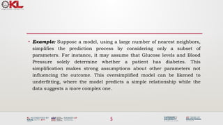
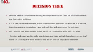
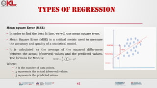
• Mathematical Representation: The variance error in the
model can be mathematically expressed as:
Variancef(x)) = E[X^2] - E[X]^2
• Some examples of machine learning algorithms with low
variance are, Linear Regression, Logistic Regression, and
Linear discriminant analysis.
• At the same time, algorithms with high variance are decision
tree, Support Vector Machine, and K-nearest neighbours.

11. 11
VARIANCE
• Overfitting: When the model overlearns from the training data
and captures even the noise, it is said to have high variance,
resulting in overfitting.
Example:
• Consider a classification model that predicts whether a patient has
diabetes. If the model, due to high variance, makes complex and
overfitted predictions like "if the number of pregnancies is more than 3,
glucose level is more than 78, diastolic blood pressure is less than 98,
skin thickness is less than 23 mm, and so on for every feature, then
the patient has diabetes," it is prone to making inaccurate predictions
when exposed to new data. This can be costly and unreliable.

12. 12
WAYSTO REDUCE HIGHVARIANCE
• Reduce the input features or number of parameters as a model is
overfitted.
• Do not use a much complex model.
• Increase the training data.
• Increase the Regularization term.

13. BIAS-VARIANCE TRADEOFF IN
MACHINE LEARNING
• The bias-variance tradeoff is a fundamental concept in machine learning, striking a
balance between two critical sources of error: bias and variance.
• Bias represents errors due to overly simplistic model assumptions. High bias results
in underfitting, causing poor performance on training and unseen data.
• Variance reflects the model's sensitivity to fluctuations in the training data. High
variance leads to overfitting, where the model captures noise and performs poorly on
new data.
• The goal is to find the right level of complexity in a model to minimize both bias and
variance. Achieving this balance is essential for good generalization to new data.
• 13

14. 14
DECISION TREE
• Decision Tree is a Supervised learning technique that can be used for both classification
and Regression problems.
• It is a tree-structured classifier, where internal nodes represent the features of a dataset,
branches represent the decision rules and each leaf node represents the outcome.
• In a Decision tree, there are two nodes, which are the Decision Node and Leaf Node.
• Decision nodes are used to make any decision and have multiple branches, whereas Leaf
nodes are the output of those decisions and do not contain any further branches.

15. • The decisions or the test are performed
on the basis of features of the given
dataset.
• It is a graphical representation for getting
all the possible solutions to a
problem/decision based on given
conditions.
15

16. 16
WHY USE DECISION TREES
• Decision Trees usually mimic human thinking ability while making a decision, so it is easy to understand.
• The logic behind the decision tree can be easily understood because it shows a tree-like structure.
Decision Tree Terminologies
• Root Node: Root node is from where the decision tree starts. It represents the entire dataset, which further gets divided into
two or more homogeneous sets.
• Leaf Node: Leaf nodes are the final output node, and the tree cannot be segregated further after getting a leaf node.
• Splitting: Splitting is the process of dividing the decision node/root node into sub-nodes according to the given conditions.
• Branch/Sub Tree: A tree formed by splitting the tree.
• Pruning: Pruning is the process of removing the unwanted branches from the tree.
• Parent/Child node: The root node of the tree is called the parent node, and other nodes are called the child nodes.

17. 17
Decision tree representation
A decision tree for whether to approve a loan.
Employed?
Credit score? Income?
Approve Reject Approve Reject
No Yes
High High
Low Low

18. 19
Decision tree for play tennis
Day Outlook Temperature Humidity Wind PlayTennis
1 Sunny Hot High Weak No
2 Sunny Hot High Strong No
3 Overcast Hot High Weak Yes
4 Rain Mild High Weak Yes
5 Rain Cool Normal Weak Yes
6 Rain Cool Normal Strong No
7 Overcast Cool Normal Strong Yes
8 Sunny Mild High Weak No
9 Sunny Cool Normal Weak Yes
10 Rain Mild Normal Weak Yes
11 Sunny Mild Normal Strong Yes
12 Overcast Mild High Strong Yes
13 Overcast Hot Normal Weak Yes
14 Rain Mild High Strong No

19. 20
Decision tree for play tennis
• Attributes and their values:
• Outlook: Sunny, Overcast, Rain
• Temperature: Hot, Mild, Cool
• Humidity: High, Normal
• Wind: Strong, Weak
• Target:
• Play Tennis: Yes, No
Day
Outloo
k
Temperatu
re
Humidi
ty
Wind
Play
Tennis
1 Sunny Hot High Weak No
2 Sunny Hot High Strong No
3 Overcast Hot High Weak Yes
4 Rain Mild High Weak Yes
5 Rain Cool Normal Weak Yes
6 Rain Cool Normal Strong No
7 Overcast Cool Normal Strong Yes
8 Sunny Mild High Weak No
9 Sunny Cool Normal Weak Yes
10 Rain Mild Normal Weak Yes
11 Sunny Mild Normal Strong Yes
12 Overcast Mild High Strong Yes
13 Overcast Hot Normal Weak Yes
14 Rain Mild High Strong No

20. 21
Decision tree for play tennis
Outlook
Humidity Wind
High Normal Strong Weak
Sunny Overcast Rain
Yes
Yes
NO Yes
NO

21. 22
ID3 algorithm
• ID3 is a basic decision tree learning algorithm.
• ID3 stands for Iterative Dichotomiser 3.
• The ID3 algorithm was invented by Ross Quinlan in 1975.
• Used to generate a decision tree from a given data set by employing a top-down, greedy
search, to test each attribute at every node of the tree.
• The resulting tree is used to classify future samples.
• It is a classification algorithm that follows a greedy approach by selecting a best attribute
that yields maximum Information Gain (G) or minimum Entropy (S).

22. 23
ID3 algorithm
• Create a Root node for the tree
• If all Examples are positive, Return the single-node tree Root, with label = +
• If all Examples are negative, Return the single-node tree Root, with label = -
• If Attributes is empty, Return the single-node tree Root, with label = most common value of
Target_attribute in Examples.

23. 24
ID3 algorithm
• Otherwise Begin
• A ← the attribute from Attributes that best* classifies Examples
• The decision attribute for Root ← A
• For each possible value, vi, of A,
• Add a new tree branch below Root, corresponding to the test A = vi
• Let Examples vi, be the subset of Examples that have value vi for A
• If Examples vi , is empty
• Then below this new branch add a leaf node with label = most common value of
Target_attribute in Examples
• Else below this new branch add the subtree
ID3(Examples vi, Targe_tattribute, Attributes – {A}))
• End
• Return Root

24. 25
Which attribute is the best
classifier?
• The central choice in the ID3 algorithm is selecting which attribute to test at each node in the
tree.
• A statistical property called information gain that measures how well a given attribute separates
the training examples according to their target classification.
• Information Gain= Entropy(S)- [(Weighted Avg) *Entropy(each feature)
• ID3 uses this information gain measure to select among the candidate attributes at each step
while growing the tree.
• In order to define information gain precisely, we use a measure commonly used in
information theory, called entropy.

25. 26
Entropy
• Entropy: Entropy is a metric to measure the impurity in a given attribute.
• It specifies randomness in data. Entropy can be calculated as:
• Given a collection S, containing positive and negative examples of some target
concept,
the entropy of S relative to this Boolean classification is
Where,
• p+ is the proportion of positive examples in S.
• p- is the proportion of negative examples in S.
Entropy(s)= -P(yes)log2 P(yes)- P(no) log2 P(no)
Where,
S=Total number of samples
P(yes)= probability of yes
P(no)= probability of no

26. 27
Information gain
• Information gain, is the expected reduction in entropy caused by partitioning the
examples according to this attribute.
• The information gain, Gain(S, A) of an attribute A, relative to a collection of
examples S, is defined as

27. 28
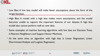
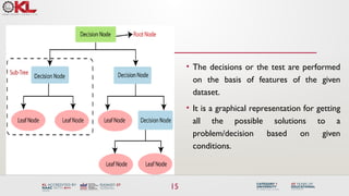
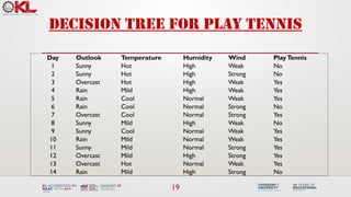
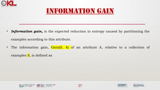
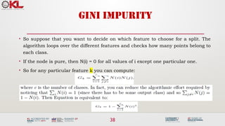
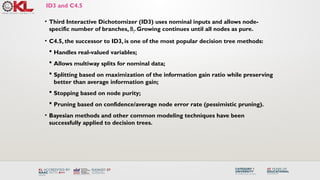
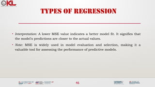
Which attribute is the best classifier?
A1=?
True False
[21+, 5-] [8+, 30-]
[29+,35-]
A2=?
True False
[18+, 33-] [11+, 2-]
[29+,35-]

28. 29
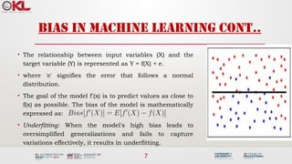
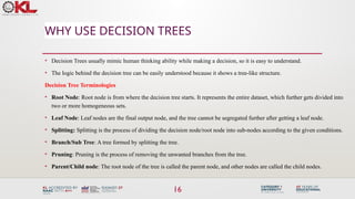
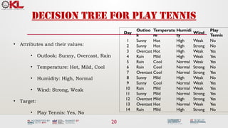
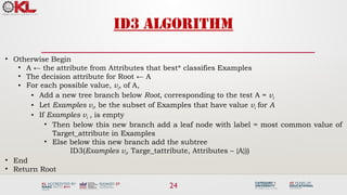
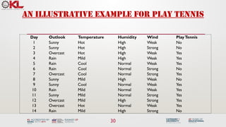
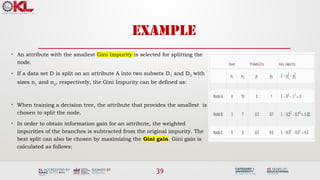
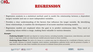
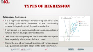
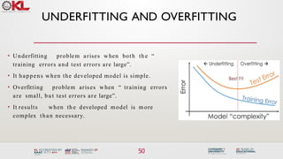
Which attribute is the best classifier?
𝐸𝑛𝑡𝑟𝑜𝑝𝑦 ([ 29+ , 35 −] )=−
29
64
log2
29
64
−
35
64
log 2
35
64
=0.99
•
0.12
•
0.27
• A1 provides greater information gain than A2, So A1 is a better classifier than A2.

29. 30
An illustrative example for play tennis
Day Outlook Temperature Humidity Wind PlayTennis
1 Sunny Hot High Weak No
2 Sunny Hot High Strong No
3 Overcast Hot High Weak Yes
4 Rain Mild High Weak Yes
5 Rain Cool Normal Weak Yes
6 Rain Cool Normal Strong No
7 Overcast Cool Normal Strong Yes
8 Sunny Mild High Weak No
9 Sunny Cool Normal Weak Yes
10 Rain Mild Normal Weak Yes
11 Sunny Mild Normal Strong Yes
12 Overcast Mild High Strong Yes
13 Overcast Hot Normal Weak Yes
14 Rain Mild High Strong No

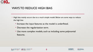
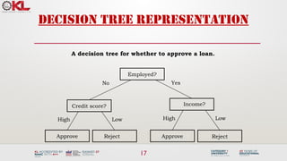
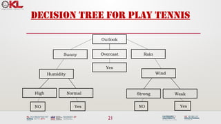
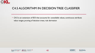
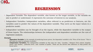
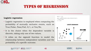
30. Selecting next attribute
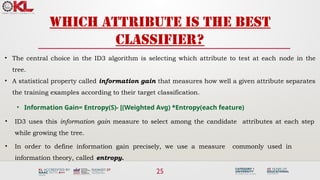
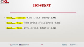
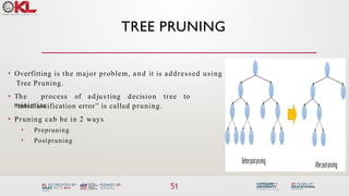
• Entropy([9+,5-] = – (9/14) log2(9/14) – (5/14) log2(5/14) = 0.940
Sunny Rain
S=[9+,5-]
E=0.940
[2+, 3-]
E=0.971
[3+, 2-]
E=0.971
Gain(S, Outlook) = 0.940-(5/14)*0.971 -(4/14)*0.0
-(5/14)*0.0971
= 0.247
Overcast
[4+, 0]
E=0.0
Hot Cold
S=[9+,5-]
E=0.940
[2+, 2-]
E=1.0
[3+, 1-]
E=0.811
Gain(S, Temp) = 0.940-(4/14)*1.0 - (6/14)*0.911
- (4/14)*0.811
= 0.029
Mild
[4+, 2-]
E= 0.911
Outlook Temperature

31. 32
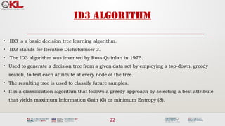
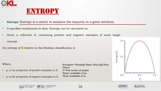
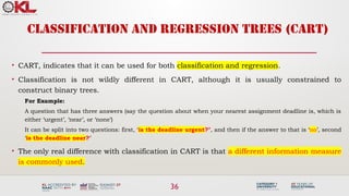
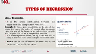
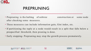
Selecting next attribute
Humidity
High Normal
[3+, 4-] [6+, 1-]
S=[9+,5-]
E=0.940
Gain(S, Humidity) = 0.940-(7/14)*0.985-(7/14)*0.592
= 0.151
E=0.592
Wind
Weak Strong
[6+, 2-] [3+, 3-]
S=[9+,5-]
E=0.940
Gain(S, Wind) = 0.940-(8/14)*0.811-(6/14)*1.0
= 0.048
E=0.985

32. 33
Best attribute-outlook
• The information gain values for the 4 attributes are:
• Gain(S, Outlook) = 0.247
• Gain(S, Temp) = 0.029
• Gain(S, Humidity) = 0.151
• Gain(S, Wind) = 0.048
Sunny Rain
[2+, 3-]
S=[9+,5-]
S={D1,D2,…,D14}
Overcast
[3+, 2-]
Srain={D4,D5,D6,D10,D14}
[4+, 0]
Sovercast={D3,D7,D12,D13}
Which attribute should be tested here?
Outlook
Yes
? ?
Ssunny={D1,D2,D8,D9,D11}

33. 34
ID3-sunny
• Gain(Ssunny , Humidity) = 0.970-(3/5)0.0 – 2/5(0.0) = 0.970
• Gain(Ssunny , Temp.) = 0.970-(2/5)0.0 –2/5(1.0)-(1/5)0.0 = 0.570
• Gain(Ssunny , Wind) = 0.970= -(2/5)1.0 – 3/5(0.918) = 0.019

34. 35
ID3-result
Outlook
Sunny Overcast Rain
Humidity
[D3,D7,D12,D13]
Strong Weak
Yes
Yes
[D8,D9,D11]
No
[D6,D14]
Yes
[D4,D5,D10]
No
[D1,D2]
High Normal
Wind

35. 36
CLASSIFICATION AND REGRESSION TREES (CART)
• CART, indicates that it can be used for both classification and regression.
• Classification is not wildly different in CART, although it is usually constrained to
construct binary trees.
For Example:
A question that has three answers (say the question about when your nearest assignment deadline is, which is
either ‘urgent’, ‘near’, or ‘none’)
It can be split into two questions: first, ‘is the deadline urgent?’, and then if the answer to that is ‘no’, second
‘is the deadline near?’
• The only real difference with classification in CART is that a different information measure
is commonly used.

36. 37
GINI IMPURITY
• The entropy that was used in ID3 as the information measure is not the only way to pick
features. Another is Gini impurity.
• The ‘impurity’ in the name suggests that the aim of the decision tree is to have each leaf
node represent a set of data-points that are in the same class. so that there are no
mismatches. This is known as purity.
• If a leaf is pure then all of the training data within it have just one class.
In which case, if we count the number of data points at the node, that belong to a class i (call it
N(i)), then it should be 0 for all except one value of i.

37. 38
GINI IMPURITY
• So suppose that you want to decide on which feature to choose for a split. The
algorithm loops over the different features and checks how many points belong to
each class.
• If the node is pure, then N(i) = 0 for all values of i except one particular one.
• So for any particular feature k you can compute:

38. 39
EXAMPLE
• An attribute with the smallest Gini Impurity is selected for splitting the
node.
• If a data set D is split on an attribute A into two subsets D1 and D2 with
sizes n1 and n2, respectively, the Gini Impurity can be defined as:
• When training a decision tree, the attribute that provides the smallest is
chosen to split the node.
• In order to obtain information gain for an attribute, the weighted
impurities of the branches is subtracted from the original impurity. The
best split can also be chosen by maximizing the Gini gain. Gini gain is
calculated as follows:

39. 40
C4.5 ALGORITHM IN DECISION TREE CLASSIFIER
• C4.5 is an extension of ID3 that accounts for unavailable values, continuous attribute
value ranges, pruning of decision trees, rule derivation

40. ID3 and C4.5
• Third Interactive Dichotomizer (ID3) uses nominal inputs and allows node-
specific number of branches, Bj. Growing continues until all nodes as pure.
• C4.5, the successor to ID3, is one of the most popular decision tree methods:
 Handles real-valued variables;
 Allows multiway splits for nominal data;
 Splitting based on maximization of the information gain ratio while preserving
better than average information gain;
 Stopping based on node purity;
 Pruning based on confidence/average node error rate (pessimistic pruning).
• Bayesian methods and other common modeling techniques have been
successfully applied to decision trees.

41. 42
REGRESSION
• Regression analysis is a statistical method used to model the relationship between a dependent
(target) variable and one or more independent variables.
• Provides a clear understanding of the factors that influence the target variable. By identifying
these relationships, it enables the development of accurate machine learning models.
• Regression models are employed when the goal is to predict continuous data. They excel at
estimating values within a range, making them valuable in various domains.
Example:
• Predicting Rainfall: Rainfall can depend on various factors, including humidity, temperature, wind direction, and wind
speed. A regression model can help forecast rainfall amounts based on these variables.
• Predicting House Prices: The price of a house in a certain area may be influenced by a multitude of factors, such as
size, locality, distance to schools, hospitals, metro stations, marketplaces, pollution levels, and the presence of parks. A
regression model can take these variables into account to estimate house prices accurately.

42. 43
REGRESSION
• Dependent Variable: The dependent variable, also known as the target variable, is the variable we
aim to predict or understand. It represents the outcome of interest in our analysis.
• Independent Variables: Independent variables, often referred to as predictors or features, are the
variables used to predict the values of the dependent variable. They serve as the input values in a
predictive model.
• Independent variables can be thought of as the inputs, while the dependent variable is the output
of these inputs. The relationships between the independent and dependent variables are the core of
regression analysis.
Example:
• Dependent Variable: In the example of predicting house prices, the dependent variable is the "Price of the house." This is
the value we want to estimate or predict.
• Independent Variables: The independent variables in this case are "size," "Locality," "distance from school, hospital,
metro, and market," "pollution level," and "number of parks." These are the factors that influence or help predict the
house price.

43. 44
TYPES OF REGRESSION
Linear Regression
• It is the linear relationship between the
dependent and independent variables.
Example: In house price prediction, as the size of the
house increases, the price of houses also increases.
Here, the size of the house is an independent variable
and the price of a house is a dependent variable.
• In a linear regression model, we try to find the best fit
line (i.e. the best value of m and c) to reduce the error.
• Note:Error is the difference between the actual
value and the predictive value.

44. 45
TYPES OF REGRESSION
Mean square Error (MSE)
• In order to find the best fit line, we will use mean square error.
• Mean Square Error (MSE) is a critical metric used to measure
the accuracy and quality of a statistical model.
• It is calculated as the average of the squared differences
between the actual (observed) values and the predicted values.
The formula for MSE is:
Where:
• n is the number of data points.
• y represents the actual (observed) values.
• ŷ represents the predicted values.

45. 46
TYPES OF REGRESSION
• Interpretation: A lower MSE value indicates a better model fit. It signifies that
the model's predictions are closer to the actual values.
• Note: MSE is widely used in model evaluation and selection, making it a
valuable tool for assessing the performance of predictive models.

46. 47
TYPES OF REGRESSION
Polynomial Regression
• It is a regression technique for modeling non-linear data
by fitting polynomial functions to the relationship
between independent and dependent variables.
• A polynomial is a mathematical expression consisting of
variable powers multiplied by coefficients.
• Useful for capturing complex non-linear relationships in
data, especially when points follow a curve.
• Allows the use of polynomial functions of various orders
(e.g., quadratic, cubic) to adapt to the data's curvature.

47. 48
TYPES OF REGRESSION
Logistic regression
• Logistic regression is employed when computing the
probability of mutually exclusive events, such as
True/False, Pass/Fail, 0/1, or Yes/No.
• It is the choice when the dependent variable is
discrete, taking only one of two values.
• It relies on the sigmoid function to model the
relationship between independent variables and the
probability of a specific outcome.

48. CHALLENGES IN DECISION TREE CLASSIFICATION
49
• Decision Trees are mainly made to classify the item set.
• While classifying we observed 2 problems.
• Underfitting
• Overfitting

49. UNDERFITTING AND OVERFITTING
• Underfitting problem arises when both th e “
training errors and test errors are large”.
• It happens when the developed model is simple.
• Overfitting problem arises when “ training errors
are small, but test errors are large”.
• It results when th e developed model is m ore
complex than necessary.
50

50. TREE PRUNING
• Overfitting is the major problem, and it is addressed using
Tree Pruning.
51
• The process of adju s ting decision tree to
minimize
“misclassification error” is called pruning.
• Pruning cab be in 2 ways
• Prepruning
• Postpruning

51. PREPRUNING
52
• Prepruning is the halting of subtree construction at some node
after checking some measures.
• These measures can include information gain, Gini index, etc.
• If partitioning the tuple at a node would result in a split that falls below a
prespecified threshold, then pruning is done.
• Early stopping- Prepruning may stop the growth process prematurely.

52. POSTPRUNING
53
• The decision tree has initially grown to its maximum size.
• Then examine each branch.
• Trim the nodes of the decision tree in a bottom-up fashion
• Post pruning is done by replacing the node with a leaf.
• If the error improves after trimming, replace the sub-tree with a leaf node.
• Post-pruning is more computationally expensive than prepruning because
the entire tree is grown.

53. 54
Self-Assessment Questions
1. Which of the following is a crucial step in designing a machine learning system?
(a) Selecting a programing language
(b) Choosing a machine learning algorithm randomly
(c) Skipping the evaluation phase
(d) Collecting and preparing a high-quality dataset
2. What is the purpose of feature engineering in machine learning system design?
(a) To automate the model training process
(b) To select the best machine learning algorithm
(c) To extract and transform raw data into informative features
(d) To validate the performance of the machine learning model

54. 55
Self-Assessment Questions
1. What does a high variance in a machine learning model indicate?
A) The model makes overly simplistic assumptions.
B) The model overlearns from the training data.
C) The model underfits the data.
D) The model balances bias and variance effectively.
2. Which of the following strategies is NOT typically used to manage high bias in a machine learning
model?
A) Regularization techniques.
B) Feature selection.
C) Increasing model complexity.
D) Ensemble methods.

55. 56
REFERENCES FOR FURTHER LEARNING OF THE SESSION
Text Books:
1. Mitchell, Tom. Machine Learning. New York, NY: McGraw-Hill, 1997. ISBN: 9780070428072.
2. MacKay, David. Information Theory, Inference, and Learning Algorithms. Cambridge, UK: Cambridge University Press,
2003. ISBN: 9780521642989.
Reference Books:
3. EthemAlpaydin “Introduction to Machine Learning “, The MIT Press (2010).
4. Stephen Marsland, “Machine Learning an Algorithmic Perspective” CRC Press, (2009).
Sites andWeb links:
5. Data Science and Machine Learning: https://www.edx.org/course/data-science-machinelearning.
2. Machine Learning: https://www.ocw.mit.edu/courses/6-867-machine-learning-fall-2006/.

56. 57
THANK YOU
Team – MACHINE LEARNING