1. You are given only three quarterly seasonal indices and quarterly seasonally adjusted data for the entire year.  What is the raw data value for Q4?  Raw data is not adjusted for seasonality. Quarter   Seasonal  Index             Seasonally Adjusted Data Q1              .80                               295 Q2              .85                               299 Q3             1.15                              270 Q4              ---                                271 (Points : 3)  325         225         252         271 Question 2. 2. One model of exponential smoothing will provide almost the same forecast as a liner trend method.  What are linear trend intercept and slope counterparts for exponential smoothing? (Points : 3) Alpha and Delta Delta and Gamma Alpha and Gamma Std Dev and Mean Question 3. 3. Why is the residual mean value important to a forecaster? (Points : 3)  Large mean values indicate nonautoregressiveness.         Small mean values indicate the total amount of error is small.       Large absolute mean values indicate estimate bias.  Large mean values indicate the standard error of the model is small. Question 4. 4. When performing correlation analysis what is the null hypothesis?  What measure in Minitab is used to test it and to be 95% confident in the significance of correlation coefficient. (Points : 3) Ho:  r = .05    p < .5 Ho:  r = 1     p =.05 Ho:  r ≠ 0      p≤.05 Ho: r = 0       p≤.05 Question 5. 5. In decomposition what does the cycle factor (CF) of .80 represent for a monthly forecast estimate of a Y variable? (Points : 3)  The estimated value is 80% of the average monthly seasonal estimate.         The estimate is .80 of the forecasted Y trend value.         The estimated value is .80 of the historical average CMA values.         The estimated value has 20% more variation than the average historical Y data values. Question 6. 6. A Burger King franchise owner notes that the sales per store has fallen below the stated national Burger King outlet average of $1,258,000.  He asserts a change has occurred that reduced the fast food eating habits of Americans.  What is his hypothesis (H1) and what type of test for significance must be applied? (Points : 3)  H1: u ≥ $1.258,000  A one-tailed t-test to the left.         H1:  u = $1.258,000 A two-tailed t-test.         H1:  u < $1.258,000 A one-tailed t-test to the left.         H1:  p < $1.258,000 A one-tailed test to the right. Question 7. 7. The CEO of Home Depot wants to see if city size has any relationship to the current profit margins of the company stores.  What data type will he likely use to determine this? (Points : 3)  Time series data of profits by store.         Recent 10 year sample of profits by stores.         Recent cross section of store profits by city.         Trend of a random sample of store profits over time. Question 8. 8. Sometimes forecasters get lazy or forgetful and do not check the significance of XY data correlations ...

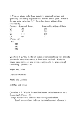
1. 1. You are given only three quarterly seasonal indices and
quarterly seasonally adjusted data for the entire year. What is
the raw data value for Q4? Raw data is not adjusted for
seasonality.
Quarter Seasonal Index Seasonally Adjusted Data
Q1 .80 295
Q2 .85 299
Q3 1.15 270
Q4 --- 271
(Points : 3)
325
225
252
271
Question 2. 2. One model of exponential smoothing will provide
almost the same forecast as a liner trend method. What are
linear trend intercept and slope counterparts for exponential
smoothing? (Points : 3)
Alpha and Delta
Delta and Gamma
Alpha and Gamma
Std Dev and Mean
Question 3. 3. Why is the residual mean value important to a
forecaster? (Points : 3)
Large mean values indicate nonautoregressiveness.
Small mean values indicate the total amount of error is

2. small.
Large absolute mean values indicate estimate bias. Large
mean values indicate the standard error of the model is small.
Question 4. 4. When performing correlation analysis what is the
null hypothesis? What measure in Minitab is used to test it and
to be 95% confident in the significance of correlation
coefficient. (Points : 3)
Ho: r = .05 p < .5
Ho: r = 1 p =.05
Ho: r ≠ 0 p≤.05
Ho: r = 0 p≤.05
Question 5. 5. In decomposition what does the cycle factor (CF)
of .80 represent for a monthly forecast estimate of a Y variable?
(Points : 3)
The estimated value is 80% of the average monthly seasonal
estimate.
The estimate is .80 of the forecasted Y trend value.
The estimated value is .80 of the historical average CMA
values.
The estimated value has 20% more variation than the
average historical Y data values.
Question 6. 6. A Burger King franchise owner notes that the
sales per store has fallen below the stated national Burger King
outlet average of $1,258,000. He asserts a change has occurred
that reduced the fast food eating habits of Americans. What is
his hypothesis (H1) and what type of test for significance must

3. be applied? (Points : 3)
H1: u ≥ $1.258,000 A one-tailed t-test to the left.
H1: u = $1.258,000 A two-tailed t-test.
H1: u < $1.258,000 A one-tailed t-test to the left.
H1: p < $1.258,000 A one-tailed test to the right.
Question 7. 7.
The CEO of Home Depot wants to see if city size has any
relationship to the current profit margins of the company
stores. What data type will he likely use to determine this?
(Points : 3)
Time series data of profits by store.
Recent 10 year sample of profits by stores.
Recent cross section of store profits by city.
Trend of a random sample of store profits over time.
Question 8. 8. Sometimes forecasters get lazy or forgetful and
do not check the significance of XY data correlations and use
the X variable to forecast Y. What is the result of this?
(Points : 3)
Type 2 error
Autocorrelation error
Type 3 error
Type 1 error
Question 9. 9. In exponential smoothing what is the weight of
the alpha coefficient for a time series data observation from the
3rd previous period if the original alpha value is set at .3?
(Points : 3)
The weight cannot be calculated since the data observation is
not given.
The weight is zero since the alpha value is set relatively
high.

4. .125
.103
.084
Question 10. 10. What is not a characteristic of a random data
series? (Points : 3)
Zero mean with an normal distribution
ACF LBQ values greater than a .05 confidence level.
Non Autoregressive observations
Central tendency
Question 11. 11. What is the major cause of non randomness
(autoregressiveness) in business data? (Points : 3)
Randomness only occurs for short time periods.
Random events such as storms or technologies offset over
the long run.
Measurements naturally increase or decrease over time.
Business participant’s decisions and work.
Question 12. 12.
Given the data series below for variables Y (Monthly Inventory
Balance) and X (Monthly Sales) are they significantly
correlated at the 95% confidence level and how can you tell?
(This data also appears in the docsharing download for Exam 1
excel worksheet under the problem 12 tab.)
Ending Inv. Bal. Y
Monthly Sales X
1544
5053
1913

5. 5052
2028
7507
1178
2887
1554
3880
1910
4454
1208
3855
2467
8824
2101
5716
(Points : 3)
Yes. The correlation coefficient is .873 that is greater than
.05.
Yes. The correlation p-value is .002 which is less than .05.
No. The correlation coefficient is above the p-value.
No. The correlation p-value is greater than the 95%
confidence level.
Question 13. 13. You have forecast the sales for your company
for the last 12 months and the forecast residuals are shown
below. Are these residuals to be considered random? (This
data also appears in the docsharing excel worksheet download
for Exam 1 under the Problem 13 tab.)

6. Residuals
-24
-348
-892
-62
-378
-489
-342
34
490
23
578
198 (Points : 3)
Yes, since the residuals randomly vary in magnitude.
Yes since the residuals are positive and negative and vary
in magnitude.
No, since the residuals are stationary and vary in
magnitude.
No, since the residuals indicate positive slope.
Question 14. 14. Which form of exponential smoothing can
result in a naïve forecast? (Points : 3)
Winters with a very low seasonal coefficient.
Single with a very low trend coefficient.
Single with a very high alpha value.
Double with a very low alpha value.
Question 15. 15. What primary statistical characteristic enables
forecasters to move from uncertainty to quantifiable low risk in
the business forecasting process? (Points : 3)
Large amounts of available business data naturally create
statistical accuracy.
Although business data are not normally distributed the

7. statistics from the data are normally distributed.
Statistical forecasting technology has improved the
accuracy of models to the point that forecast will not be needed.
Statistical t and p-values determine the model accuracy.
Question 16. 16. What is used to determine the forecast model
confidence level for Exponential Smoothing and Decomposition
models? (Points : 3)
The significance level of the smoothing constants
The error measures
The residual LBQ Chi-square values
The mean of the residuals
Question 17. 17. You are responsible for forecasting your
company’s revenues for the next 24 months. You have three
years of historical monthly data and previous forecasts that
indicate that the company revenues with no obvious
seasonality have grown significantly over that time. Which
forecast method would you apply to the problem? (Points : 3)
3 period moving average
12 period moving average
Simple exponential smoothing
Double exponential smoothing
Question 18. 18. You obtained a correlation coefficient from
two data series that indicates a p-value of .97. Can you be 95%
confident that the correlation is significantly different from
zero? (Points : 3)
Yes, since the p value is above the confidence level.
Yes, since the p value is above 1 minus the confidence
level.
No, since the p-value is above the 1 minus the confidence
level.

8. No, since the data is not provided to determine true
confidence.
Question 19. 19. In decomposition the seasonal indices are the
period relationships between what two data series? (Points : 3)
Seasonal moving averages and the trend data series.
Smoothed data from centered moving averaging
(seasonally adjusted) and the original data series.
Trend data and the cycle factors.
Trend data and the original data series.
Question 20. 20. If you have trend in a data series how can
you confirm it and determine if it is statistically significant"
(Points : 3)
Autocorrelation functions that spike in the 4th and 8th quarters
and have LBQ values below the LBQ table values.
A time series plot that shows the data rising and falling.
Histogram that shows the data centered around a zero mean
value with a normal distribution.
Autocorrelation functions that step down toward zero and have
LBQ values above the Chi-square tables values.
Question 21. 21. Golfsmith a sporting goods company requires
an eight quarter sales forecast. From the revenue data below
(also found in Doc Sharing under Exam 1 Data Problem 21)
what is the appropriate exponential smoothing model to apply in
order to develop the best quarterly forecast?
Date
Revenue

9. 3/31/2006
74.810
6/30/2006
114.138
9/29/2006
93.980
12/29/2006
74.962
3/30/2007
77.663
6/29/2007
124.999
9/28/2007
106.527
12/31/2007
78.969
3/31/2008
79.236
6/30/2008
129.995
9/30/2008
101.702
12/31/2008
67.840
3/31/2009
68.793
6/30/2009
114.797
9/30/2009
90.586
12/31/2009
63.850
3/31/2010
67.649
6/30/2010
118.046

10. 9/30/2010
93.272
12/31/2010
72.885
3/31/2011
81.515
6/30/2011
130.220
9/30/2011
100.997
12/30/2011
74.535
3/30/2012
90.456
(Points : 4)
Double Exponential Smoothing (Holt's)
Single Exponential Smoothing
4 Period Moving Average
Winter's Exponential Smoothing
Linear Trend
Question 22. 22. Run the data with the exponential smoothing
model that applies and obtain the best model by adjusting each
of the coefficients. (Do not use Optimal ARIMA to find the
smoothing coefficients. Make sure that you only
use one decimal place for each coefficient – e.g. .1, or .2, or .3
…. through .9.) What coefficient values will result in the best
exponential smoothing result and the lowest error? (Points : 4)
.9 level, .8 trend, .9 seasonal
.9 level, .5 trend
.9 level, .1 trend, .1 seasonal
.2 level, .6 trend, .9 seasonal
.2 level.

11. Question 23. 23. What is the RMSE for the Fit period for the
best exponential smoothing model? (Points : 4)
22.63
3.75
1.31
14.06
142.76
Question 24. 24. Use the best exponential smoothing model to
generate a forecast for 8 quarters. What is the forecast value
for the 8th quarter? (Points : 4)
28.1
85.1
60.4
46.8
75.3
Question 25. 25. The Fit period residuals from the best
exponential smoothing model are autocorrelated through the
12th lag. (Points : 4)
True
False
Question 26. 26. Use the same quarterly Golfsmith sales data
series and run a decomposition model and estimate 8 forecast
periods. Which quarter has the greatest seasonal sales? (Points
: 4)
Quarter 1
Quarter 2
Quarter 4
Quarter 3

12. Question 27. 27. What is the decomposition forecast value for
the 8th period (last forecast quarter). Be sure to adjust the
forecast with the most recent (last) cycle factor. (Points : 4)
65.0
61.5
103.8
58.2
73.2
Question 28. 28.
Are the decomposition fit period residuals random? Why or
why not?
(Points : 4)
No. They still have seasonality.
No. They still have significant cycle.
Yes. They are normally distributed with a near zero mean.
Yes. None of the residuals are significantly
autoregressive.
Question 29. 29. Based on your analysis of the best exponential
smoothing and cycle adjusted decomposition forecast MAPE
and residual analysis which model produces the best results and
why? (Points : 4)
The exponential smoothing model forecast is best since it
picked up cycle better than the adjusted decomposition forecast
and produced more random residuals.
The decomposition forecast is best since it picks up
seasonality much better than the exponential smoothing model

13. and produces high Chi-square values.
The exponential smoothing model is best since it has
lower error measures than the decomposition model forecast and
is, therefore, more accurate.
The decomposition model forecast is best since the
forecast is closer to the Hold Out and it produced lower error
for the forecast period.
Question 30. 30. Forecast error measures and residual analysis
can only be used where quantitative forecast methods and
models are applied to data. (Points : 4)
True
False
1. You are given only three quarterly seasonal indices and
quarterly seasonally adjusted data for the entire year. What is
the raw data value for Q4? Raw data is not adjusted for
seasonality.
Quarter Seasonal Index Seasonally Adjusted Data
Q1 .80 295
Q2 .85 299
Q3 1.15 270
Q4 --- 271
(Points : 3)
325
225
252
271

14. Question 2. 2. One model of exponential smoothing will provide
almost the same forecast as a liner trend method. What are
linear trend intercept and slope counterparts for exponential
smoothing? (Points : 3)
Alpha and Delta
Delta and Gamma
Alpha and Gamma
Std Dev and Mean
Question 3. 3. Why is the residual mean value important to a
forecaster? (Points : 3)
Large mean values indicate nonautoregressiveness.
Small mean values indicate the total amount of error is
small.
Large absolute mean values indicate estimate bias. Large
mean values indicate the standard error of the model is small.
Question 4. 4. When performing correlation analysis what is the
null hypothesis? What measure in Minitab is used to test it and
to be 95% confident in the significance of correlation
coefficient. (Points : 3)
Ho: r = .05 p < .5
Ho: r = 1 p =.05
Ho: r ≠ 0 p≤.05
Ho: r = 0 p≤.05

15. Question 5. 5. In decomposition what does the cycle factor (CF)
of .80 represent for a monthly forecast estimate of a Y variable?
(Points : 3)
The estimated value is 80% of the average monthly seasonal
estimate.
The estimate is .80 of the forecasted Y trend value.
The estimated value is .80 of the historical average CMA
values.
The estimated value has 20% more variation than the
average historical Y data values.
Question 6. 6. A Burger King franchise owner notes that the
sales per store has fallen below the stated national Burger King
outlet average of $1,258,000. He asserts a change has occurred
that reduced the fast food eating habits of Americans. What is
his hypothesis (H1) and what type of test for significance must
be applied? (Points : 3)
H1: u ≥ $1.258,000 A one-tailed t-test to the left.
H1: u = $1.258,000 A two-tailed t-test.
H1: u < $1.258,000 A one-tailed t-test to the left.
H1: p < $1.258,000 A one-tailed test to the right.
Question 7. 7.
The CEO of Home Depot wants to see if city size has any
relationship to the current profit margins of the company
stores. What data type will he likely use to determine this?
(Points : 3)
Time series data of profits by store.
Recent 10 year sample of profits by stores.
Recent cross section of store profits by city.
Trend of a random sample of store profits over time.

16. Question 8. 8. Sometimes forecasters get lazy or forgetful and
do not check the significance of XY data correlations and use
the X variable to forecast Y. What is the result of this?
(Points : 3)
Type 2 error
Autocorrelation error
Type 3 error
Type 1 error
Question 9. 9. In exponential smoothing what is the weight of
the alpha coefficient for a time series data observation from the
3rd previous period if the original alpha value is set at .3?
(Points : 3)
The weight cannot be calculated since the data observation is
not given.
The weight is zero since the alpha value is set relatively
high.
.125
.103
.084
Question 10. 10. What is not a characteristic of a random data
series? (Points : 3)
Zero mean with an normal distribution
ACF LBQ values greater than a .05 confidence level.
Non Autoregressive observations
Central tendency
Question 11. 11. What is the major cause of non randomness
(autoregressiveness) in business data? (Points : 3)
Randomness only occurs for short time periods.
Random events such as storms or technologies offset over
the long run.

17. Measurements naturally increase or decrease over time.
Business participant’s decisions and work.
Question 12. 12.
Given the data series below for variables Y (Monthly Inventory
Balance) and X (Monthly Sales) are they significantly
correlated at the 95% confidence level and how can you tell?
(This data also appears in the docsharing download for Exam 1
excel worksheet under the problem 12 tab.)
Ending Inv. Bal. Y
Monthly Sales X
1544
5053
1913
5052
2028
7507
1178
2887
1554
3880
1910
4454
1208
3855
2467

18. 8824
2101
5716
(Points : 3)
Yes. The correlation coefficient is .873 that is greater than
.05.
Yes. The correlation p-value is .002 which is less than .05.
No. The correlation coefficient is above the p-value.
No. The correlation p-value is greater than the 95%
confidence level.
Question 13. 13. You have forecast the sales for your company
for the last 12 months and the forecast residuals are shown
below. Are these residuals to be considered random? (This
data also appears in the docsharing excel worksheet download
for Exam 1 under the Problem 13 tab.)
Residuals
-24
-348
-892
-62
-378
-489
-342
34
490
23
578
198 (Points : 3)
Yes, since the residuals randomly vary in magnitude.
Yes since the residuals are positive and negative and vary
in magnitude.
No, since the residuals are stationary and vary in
magnitude.

19. No, since the residuals indicate positive slope.
Question 14. 14. Which form of exponential smoothing can
result in a naïve forecast? (Points : 3)
Winters with a very low seasonal coefficient.
Single with a very low trend coefficient.
Single with a very high alpha value.
Double with a very low alpha value.
Question 15. 15. What primary statistical characteristic enables
forecasters to move from uncertainty to quantifiable low risk in
the business forecasting process? (Points : 3)
Large amounts of available business data naturally create
statistical accuracy.
Although business data are not normally distributed the
statistics from the data are normally distributed.
Statistical forecasting technology has improved the
accuracy of models to the point that forecast will not be needed.
Statistical t and p-values determine the model accuracy.
Question 16. 16. What is used to determine the forecast model
confidence level for Exponential Smoothing and Decomposition
models? (Points : 3)
The significance level of the smoothing constants
The error measures
The residual LBQ Chi-square values
The mean of the residuals
Question 17. 17. You are responsible for forecasting your
company’s revenues for the next 24 months. You have three
years of historical monthly data and previous forecasts that

20. indicate that the company revenues with no obvious
seasonality have grown significantly over that time. Which
forecast method would you apply to the problem? (Points : 3)
3 period moving average
12 period moving average
Simple exponential smoothing
Double exponential smoothing
Question 18. 18. You obtained a correlation coefficient from
two data series that indicates a p-value of .97. Can you be 95%
confident that the correlation is significantly different from
zero? (Points : 3)
Yes, since the p value is above the confidence level.
Yes, since the p value is above 1 minus the confidence
level.
No, since the p-value is above the 1 minus the confidence
level.
No, since the data is not provided to determine true
confidence.
Question 19. 19. In decomposition the seasonal indices are the
period relationships between what two data series? (Points : 3)
Seasonal moving averages and the trend data series.
Smoothed data from centered moving averaging
(seasonally adjusted) and the original data series.
Trend data and the cycle factors.
Trend data and the original data series.
Question 20. 20. If you have trend in a data series how can
you confirm it and determine if it is statistically significant"
(Points : 3)
Autocorrelation functions that spike in the 4th and 8th quarters

21. and have LBQ values below the LBQ table values.
A time series plot that shows the data rising and falling.
Histogram that shows the data centered around a zero mean
value with a normal distribution.
Autocorrelation functions that step down toward zero and have
LBQ values above the Chi-square tables values.
Question 21. 21. Golfsmith a sporting goods company requires
an eight quarter sales forecast. From the revenue data below
(also found in Doc Sharing under Exam 1 Data Problem 21)
what is the appropriate exponential smoothing model to apply in
order to develop the best quarterly forecast?
Date
Revenue
3/31/2006
74.810
6/30/2006
114.138
9/29/2006
93.980
12/29/2006
74.962
3/30/2007
77.663
6/29/2007
124.999
9/28/2007
106.527
12/31/2007
78.969
3/31/2008
79.236

22. 6/30/2008
129.995
9/30/2008
101.702
12/31/2008
67.840
3/31/2009
68.793
6/30/2009
114.797
9/30/2009
90.586
12/31/2009
63.850
3/31/2010
67.649
6/30/2010
118.046
9/30/2010
93.272
12/31/2010
72.885
3/31/2011
81.515
6/30/2011
130.220
9/30/2011
100.997
12/30/2011
74.535
3/30/2012
90.456
(Points : 4)
Double Exponential Smoothing (Holt's)
Single Exponential Smoothing
4 Period Moving Average

23. Winter's Exponential Smoothing
Linear Trend
Question 22. 22. Run the data with the exponential smoothing
model that applies and obtain the best model by adjusting each
of the coefficients. (Do not use Optimal ARIMA to find the
smoothing coefficients. Make sure that you only
use one decimal place for each coefficient – e.g. .1, or .2, or .3
…. through .9.) What coefficient values will result in the best
exponential smoothing result and the lowest error? (Points : 4)
.9 level, .8 trend, .9 seasonal
.9 level, .5 trend
.9 level, .1 trend, .1 seasonal
.2 level, .6 trend, .9 seasonal
.2 level.
Question 23. 23. What is the RMSE for the Fit period for the
best exponential smoothing model? (Points : 4)
22.63
3.75
1.31
14.06
142.76
Question 24. 24. Use the best exponential smoothing model to
generate a forecast for 8 quarters. What is the forecast value
for the 8th quarter? (Points : 4)
28.1
85.1
60.4
46.8
75.3

24. Question 25. 25. The Fit period residuals from the best
exponential smoothing model are autocorrelated through the
12th lag. (Points : 4)
True
False
Question 26. 26. Use the same quarterly Golfsmith sales data
series and run a decomposition model and estimate 8 forecast
periods. Which quarter has the greatest seasonal sales? (Points
: 4)
Quarter 1
Quarter 2
Quarter 4
Quarter 3
Question 27. 27. What is the decomposition forecast value for
the 8th period (last forecast quarter). Be sure to adjust the
forecast with the most recent (last) cycle factor. (Points : 4)
65.0
61.5
103.8
58.2
73.2
Question 28. 28.
Are the decomposition fit period residuals random? Why or
why not?
(Points : 4)
No. They still have seasonality.
No. They still have significant cycle.

25. Yes. They are normally distributed with a near zero mean.
Yes. None of the residuals are significantly
autoregressive.
Question 29. 29. Based on your analysis of the best exponential
smoothing and cycle adjusted decomposition forecast MAPE
and residual analysis which model produces the best results and
why? (Points : 4)
The exponential smoothing model forecast is best since it
picked up cycle better than the adjusted decomposition forecast
and produced more random residuals.
The decomposition forecast is best since it picks up
seasonality much better than the exponential smoothing model
and produces high Chi-square values.
The exponential smoothing model is best since it has
lower error measures than the decomposition model forecast and
is, therefore, more accurate.
The decomposition model forecast is best since the
forecast is closer to the Hold Out and it produced lower error
for the forecast period.
Question 30. 30. Forecast error measures and residual analysis
can only be used where quantitative forecast methods and
models are applied to data. (Points : 4)
True
False