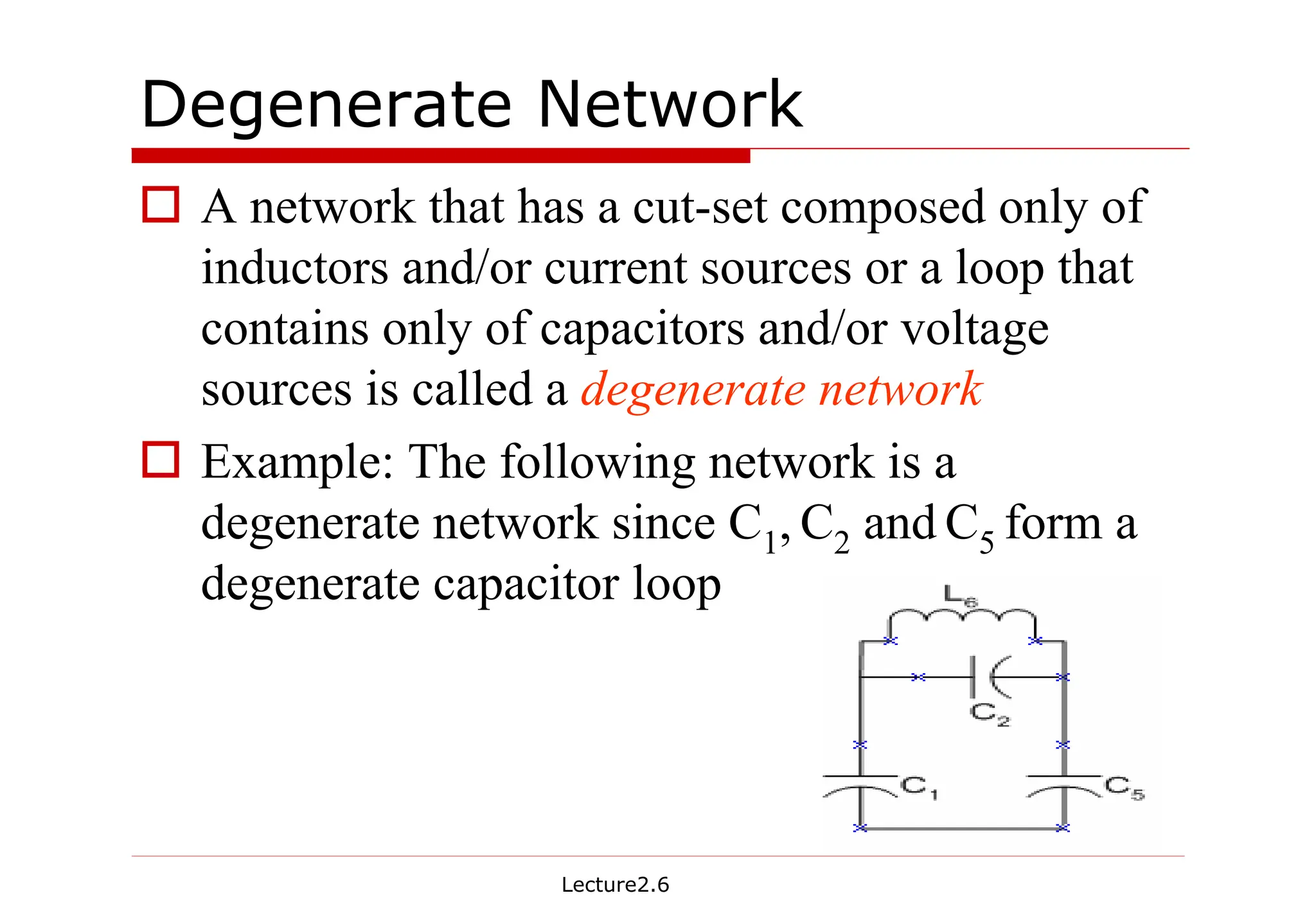
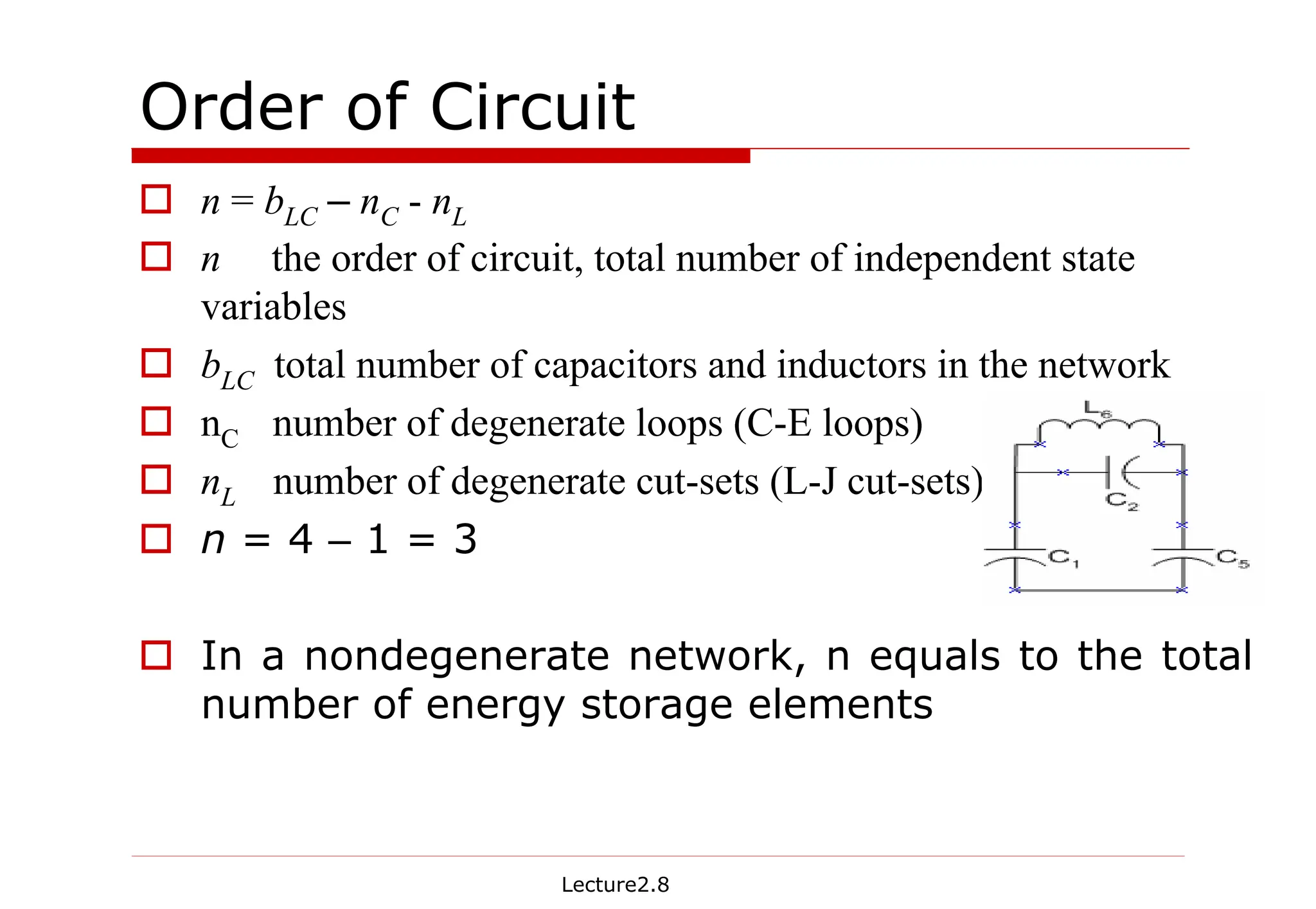
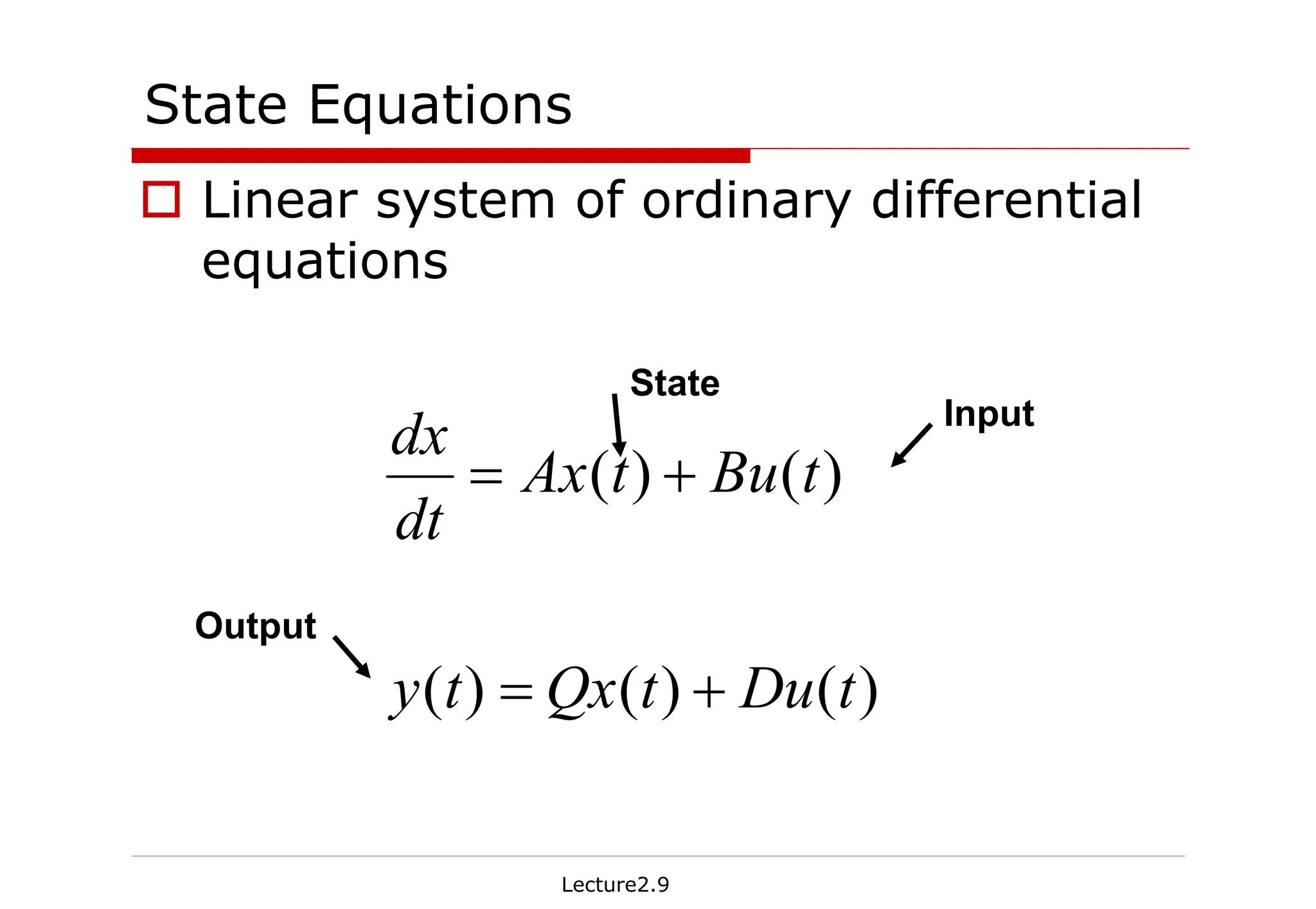
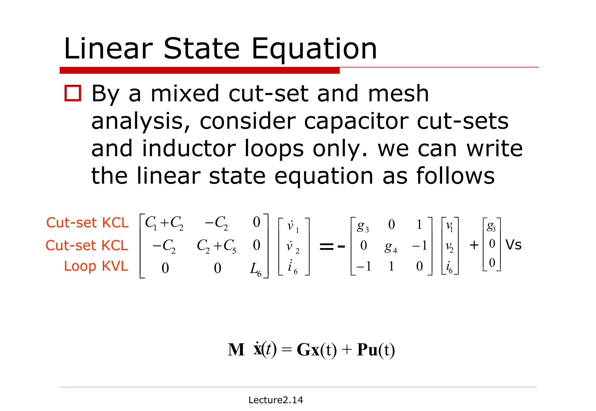
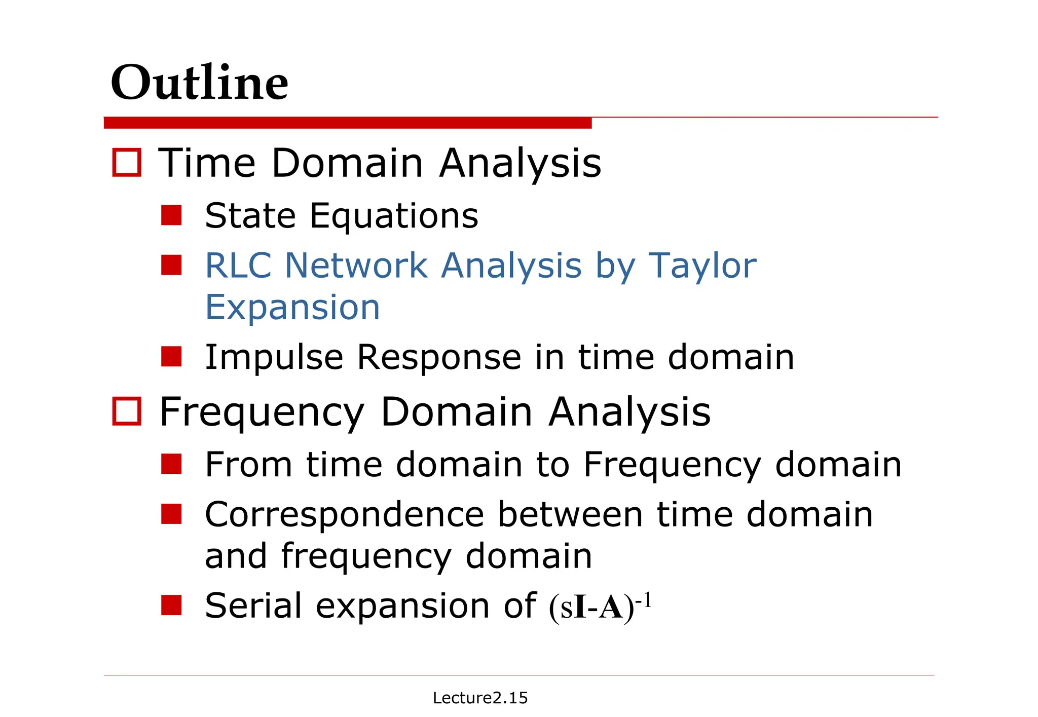
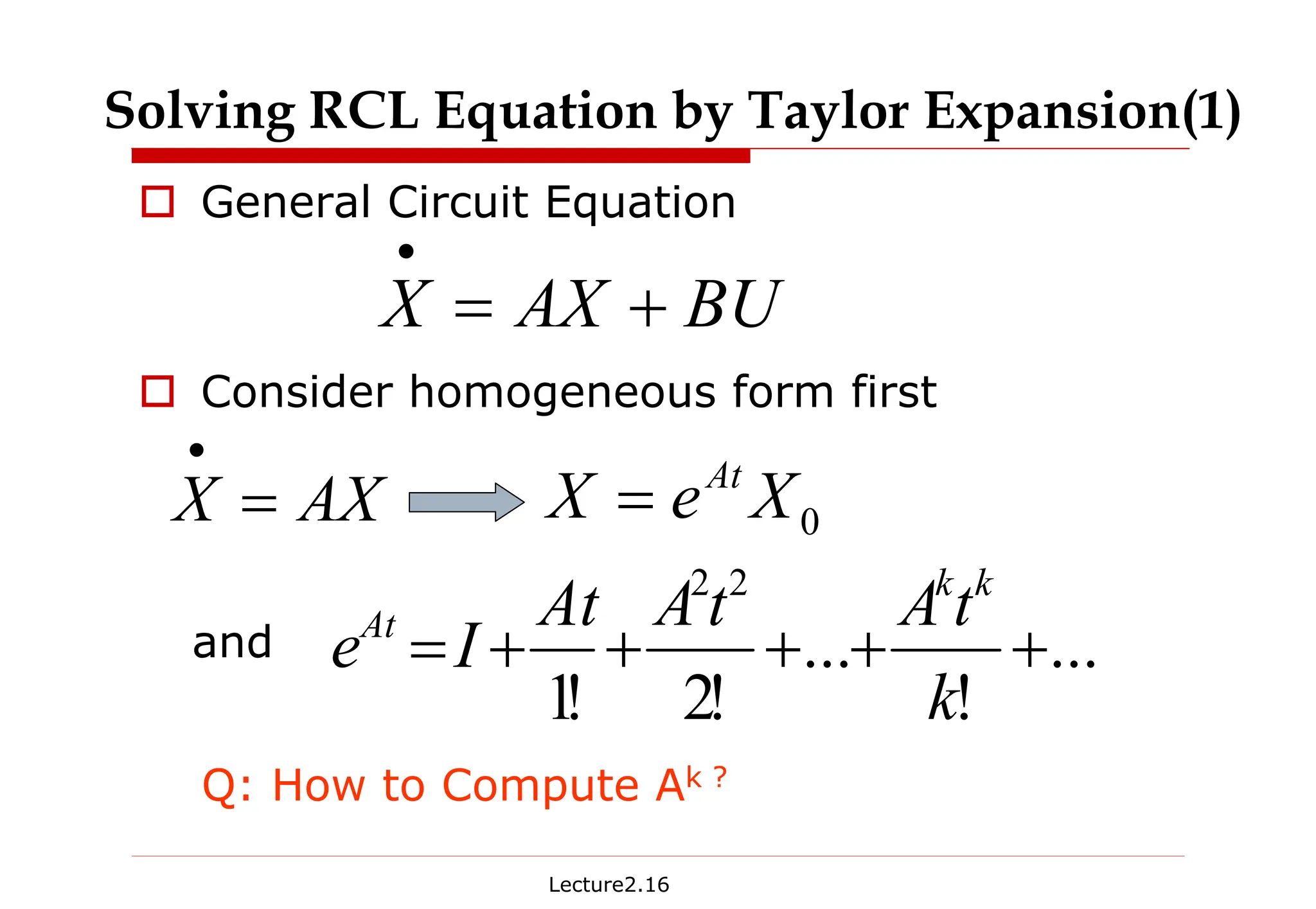
The document provides detailed lecture notes on dynamic linear system analysis, including time and frequency domain analysis, state equations, RLC network analysis, and impulse response. It discusses concepts like state variables, degenerate networks, and methods for solving RLC equations using Taylor expansion and Laplace transforms. Key examples illustrate how to derive transfer functions and the correspondence between time-domain and frequency-domain representations.

1. CSE 245: Computer Aided Circuit
Simulation and Verification
Fall 2004, Sep 28
Lecture 2:
Dynamic Linear System

2. Lecture2.2
Outline
† Time Domain Analysis
„ State Equations
„ RLC Network Analysis by Taylor
Expansion
„ Impulse Response in time domain
† Frequency Domain Analysis
„ From time domain to Frequency domain
„ Correspondence between time domain
and frequency domain
„ Serial expansion of (sI-A)-1

3. Lecture2.3
Outline (Cont’)
† Model Order Reduction
„ Moments
„ Passivity, Stability and Realizability
† Symbolic Analysis
„ Y-Delta Transformation
„ BDD Analysis

4. Lecture2.4
State of a system
† The state of a system is a set of data, the value of
which at any time t, together with the input to the
system at time t, determine uniquely the value of
any network variable at time t.
† We can express the state in vector form
x =
Where xi(t) is the state variables of the system




















)
(
.
.
.
)
(
)
(
2
1
t
x
t
x
t
x
k

5. Lecture2.5
State Variable
† How to Choose State Variable?
„ The knowledge of the instantaneous values of
all branch currents and voltages determines
this instantaneous state
„ But NOT ALL these values are required in
order to determine the instantaneous state,
some can be derived from others.
„ choose capacitor voltages and inductor
currents as the state variables! But not all of
them are chosen

6. Lecture2.6
Degenerate Network
† A network that has a cut-set composed only of
inductors and/or current sources or a loop that
contains only of capacitors and/or voltage
sources is called a degenerate network
† Example: The following network is a
degenerate network since C1, C2 and C5 form a
degenerate capacitor loop

7. Lecture2.7
Degenerate Network
† In a degenerated network, not all the capacitors
and inductors can be chosen as state variables
since there are some redundancy
† On the other hand, we choose all the capacitor
voltages and inductors currents as state variable
in a nondegenerate network
† We will give an example of how to choose state
variable in the following section

8. Lecture2.8
Order of Circuit
† n = bLC – nC - nL
† n the order of circuit, total number of independent state
variables
† bLC total number of capacitors and inductors in the network
† nC number of degenerate loops (C-E loops)
† nL number of degenerate cut-sets (L-J cut-sets)
† n = 4 – 1 = 3
† In a nondegenerate network, n equals to the total
number of energy storage elements

9. Lecture2.9
State Equations
State
Input
Output
)
(
)
(
)
(
)
(
)
(
t
Du
t
Qx
t
y
t
Bu
t
Ax
dt
dx
+
=
+
=
† Linear system of ordinary differential
equations

10. Lecture2.10
State Equation for RLC Circuits
† The state equation is of the form
† Or
† vt: voltage in the trunk, capacitor voltage
† il: current in the loop, inductor current.
† Y and R are the admittance matrix and
impedance matrix of cut-set and mesh
† E covers the co-tree branches in the cut-set
† –ET covers the tree trunks in the mesh
analysis






L
C
0
0






l
t
i
v
&
&






− R
E
E
Y
T 





l
t
i
v
= - + Pu
= Gx(t) + Pu(t)
)
(t
x
&
M

11. Lecture2.11
State Equations
† If we shift the matrix M to the right hand side, we have
† Let A = M-1G and B = M-1P, we have the state equation
† Together with the output equation
† are called the State Equations of the linear system
= Gx(t) + Pu(t)
)
(t
x
&
M
)
(t
x
& = M-1Ax(t) + M-1Bu(t)
= Ax(t) + Bu(t)
)
(t
x
&
)
(t
y = Qx(t) + Du(t)

12. Lecture2.12
RLC Network Analysis
† A given RLC network
† Degenerate Network, Choose only
voltages of C1 and C5, current of L6 as
our state variable
Vs
g3
g4
C1
C2
C5
L6
1 2
0

13. Lecture2.13
Tree Structure
† Take into tree as many capacitors as
possible and,
† as less inductors as possible
† Resistors can be chosen as either tree
branches or co-tree branches
Vs
g3
g4
C1
C2
C5
L6
1 2
0
g3
C1
C5 g4
1 2
C2
/L6
0
Vs

14. Lecture2.14
Linear State Equation
† By a mixed cut-set and mesh
analysis, consider capacitor cut-sets
and inductor loops only. we can write
the linear state equation as follows
M = Gx(t) + Pu(t)
)
(t
x
&
Cut-set KCL
Loop KVL
Cut-set KCL










+
−
−
+
6
5
2
2
2
2
1
0
0
0
0
L
C
C
C
C
C
C










6
2
1
i
v
v
&
&
&










−
−
0
1
1
1
0
1
0
4
3
g
g










6
2
1
i
v
v










0
0
3
g
=- + Vs

15. Lecture2.15
Outline
† Time Domain Analysis
„ State Equations
„ RLC Network Analysis by Taylor
Expansion
„ Impulse Response in time domain
† Frequency Domain Analysis
„ From time domain to Frequency domain
„ Correspondence between time domain
and frequency domain
„ Serial expansion of (sI-A)-1

16. Lecture2.16
Solving RCL Equation by Taylor Expansion(1)
† General Circuit Equation
† Consider homogeneous form first
BU
AX
X +
=
•
AX
X =
•
0
X
e
X At
=
...
!
...
!
2
!
1
2
2
+
+
+
+
+
=
k
t
A
t
A
At
I
e
k
k
At
Q: How to Compute Ak ?
and

17. Lecture2.17
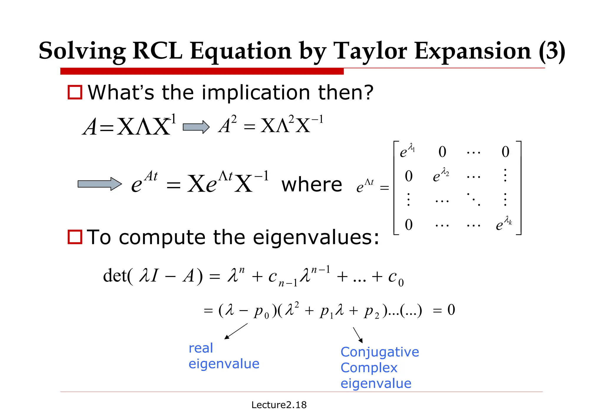
†Assume A has non-degenerate eigenvalues
and corresponding linearly
independent eigenvectors , then A
can be decomposed as
where and
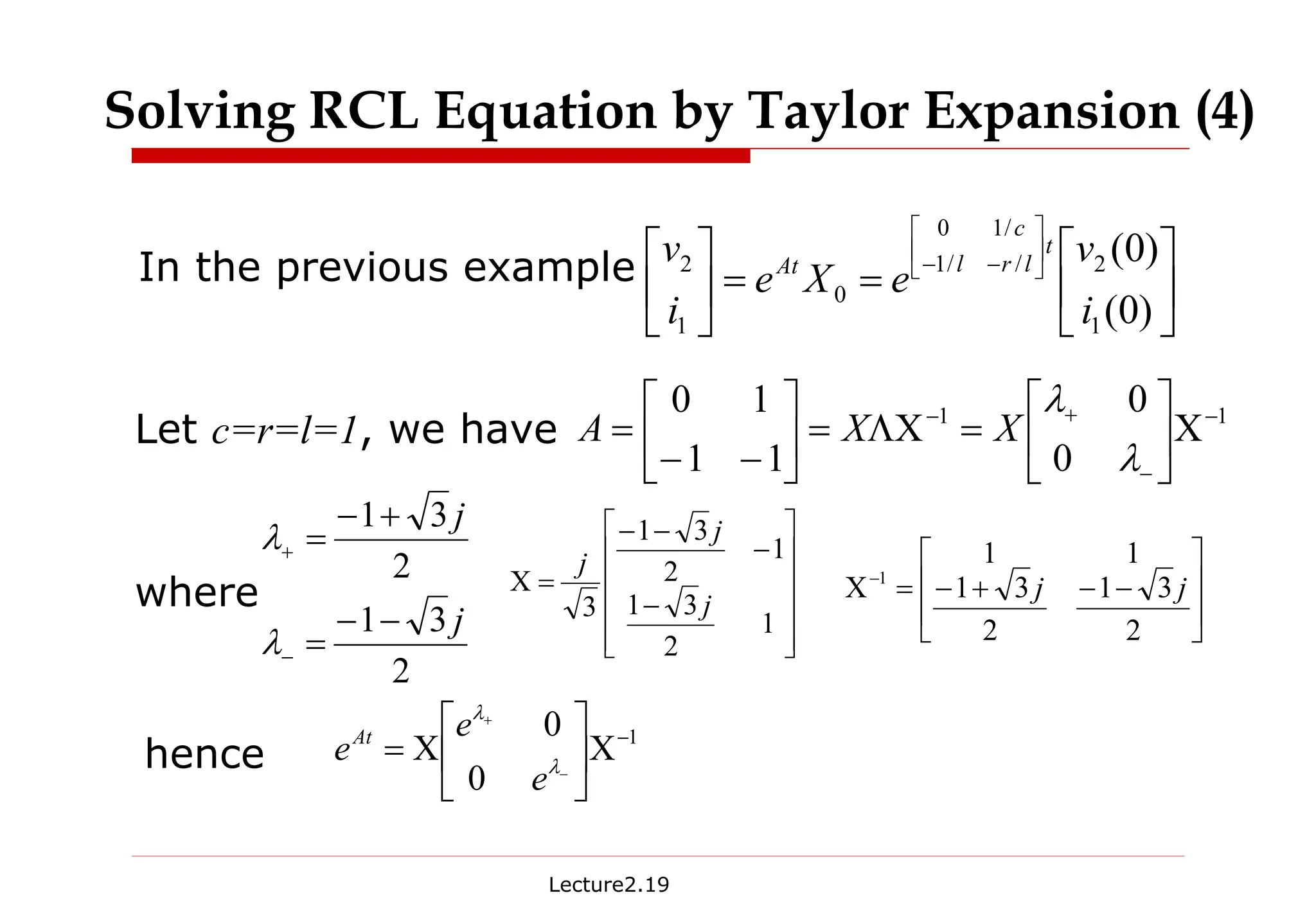
Solving RCL Equation by Taylor Expansion (2)
1
−
ΧΛΧ
=
A
k
Χ
Χ
Χ ,...,
, 2
1
k
λ
λ
λ ,...,
, 2
1












=
Λ
k
λ
λ
λ
L
L
M
O
L
M
M
L
L
0
0
0
0
2
1
[ ]
k
Χ
Χ
Χ
=
Χ ,...,
, 2
1

18. Lecture2.18
†What’s the implication then?
†To compute the eigenvalues:
1
−
ΧΛΧ
=
A
0
1
1 ...
)
det( c
c
A
I n
n
n
+
+
+
=
− −
− λ
λ
λ
0
)...(...)
)(
( 2
1
2
0 =
+
+
−
= p
p
p λ
λ
λ
real
eigenvalue
Conjugative
Complex
eigenvalue
1
2
2 −
Χ
ΧΛ
=
A
1
−
Λ
Χ
Χ
= t
At
e
e where














=
Λ
k
e
e
e
e t
λ
λ
λ
L
L
M
O
L
M
M
L
L
0
0
0
0
2
1
Solving RCL Equation by Taylor Expansion (3)

19. Lecture2.19
In the previous example






=
=





 





−
−
)
0
(
)
0
(
1
2
/
/
1
/
1
0
0
1
2
i
v
e
X
e
i
v t
l
r
l
c
At
1
1
0
0
1
1
1
0 −
−
+
−
Χ






=
ΛΧ
=






−
−
=
λ
λ
X
X
A
2
3
1
2
3
1
j
j
−
−
=
+
−
=
−
+
λ
λ
where












−
−
−
−
=
Χ
1
2
3
1
1
2
3
1
3 j
j
j








−
−
+
−
=
Χ−
2
3
1
2
3
1
1
1
1
j
j
hence
1
0
0 −
Χ






Χ
=
−
+
λ
λ
e
e
eAt
Let c=r=l=1, we have
Solving RCL Equation by Taylor Expansion (4)

20. Lecture2.20
† What if matrix A has degenerated
eigenvalues? Jordan decomposition !
1
−
Χ
Χ
= J
A
J is in the Jordan Canonical form
And still 1
−
Χ
Χ
= Jt
At
e
e
Solving RCL Equation by Taylor Expansion (5)

21. Lecture2.21
Jordan Decomposition






=
λ
λ
0
1
J 





=
+






+






= t
t
t
Jt
e
te
e
t
e λ
λ
λ
λ
λ
0
0
1
1
0
0
1
L










=
λ
λ
λ
0
0
1
0
0
1
J














=
+










+










=
t
t
t
t
t
t
Jt
e
te
e
e
t
te
e
t
e
λ
λ
λ
λ
λ
λ
λ
λ
λ
0
0
0
!
2
0
0
1
0
0
1
1
0
0
0
1
0
0
0
1
2
L
similarly

22. Lecture2.22
Outline
† Time Domain Analysis
„ State Equations
„ RLC Network Analysis by Taylor
Expansion
„ Response in time domain
† Frequency Domain Analysis
„ From time domain to Frequency domain
„ Correspondence between time domain
and frequency domain
„ Serial expansion of (sI-A)-1

23. Lecture2.23
Response in time domain
† We can solve the state equation and get the
closed form expression
† The output equation can be expressed as
Note: * denotes
convolution

24. Lecture2.24
Impulse Response
† The Impulse Response of a system is defined as
the Zero State Response resulting from an
impulse excitation
† Thus, in the output equation, replace u(t) by the
impulse function δ(t), and let x(t0)=0 we have
h(t) = y(t) = QeAt B

25. Lecture2.25
Outline
† Time Domain Analysis
„ State Equations
„ RLC Network Analysis by Taylor
Expansion
„ Impulse Response in time domain
† Frequency Domain Analysis
„ From time domain to Frequency domain
„ Correspondence between time domain
and frequency domain
„ Serial expansion of (sI-A)-1

26. Lecture2.26
Solutions in S domain
† By solving the state equation in s
domain, we have
† Suppose the network has zero state and the
output vector depends only on the state vector x,
that is, x(t0) = 0 and D = 0, we can derive the
transfer function of the network
H(s) = = Q(sI-A)-1B
x(s) = (sI-A)-1 x(t0)+ (sI-A)-1 Bu(s)
y(s) = Qx(s) +Du(s) = Q(sI-A)-1(x(t0) + Bu(s)) +Du(s)
)
(
)
(
s
s
u
y

27. Lecture2.27
Key
Key
Transform
Transform
Property:
Property:
Bilateral
Bilateral
Laplace
Laplace
Transform:
Transform:
)
(
)
(
)
(
)
(
)
(
s
Qx
s
y
s
Bu
s
Ax
s
sx
=
+
=
)
(
)
(
)
(
)
(
)
(
t
Qx
t
y
t
Bu
t
Ax
dt
t
dx
=
+
=
dt
dx
)
(s
sx
dt
e
t
x
s
x st
∫
∞
∞
−
−
= )
(
)
(
)
(t
x
Frequency Domain Representation

28. Lecture2.28
Express y(s) as a
Express y(s) as a
function of u(s)
function of u(s)
)
(
)
(
)
(
)
(
)
(
s
Qx
s
y
s
Bu
s
Ax
s
sx
=
+
=
Transfer Function:
Transfer Function: )
(s
H
)
(
)
(
)
( 1
s
Bu
A
sI
Q
s
y −
−
−
=
System Transfer Function

29. Lecture2.29
Transfer Function
Time Domain Impulse Response
Frequency domain representation
Frequency domain representation
H(s)
u(s) y(s) = H(s) u(s)
Linear system
Linear system
h(t)
u(t) ∫ −
=
t
d
u
t
h
t
y
0
)
(
)
(
)
( τ
τ
τ
Linear system
Linear system
Time domain representation
Time domain representation
The transfer function H(s) is the
The transfer function H(s) is the Laplace
Laplace Transform
Transform
of the impulse response h(t)
of the impulse response h(t)

30. Lecture2.30
Outline
† Time Domain Analysis
„ State Equations
„ RLC Network Analysis by Taylor
Expansion
„ Impulse Response in time domain
† Frequency Domain Analysis
„ From time domain to Frequency domain
„ Correspondence between time domain
and frequency domain
„ Serial expansion of (sI-A)-1

31. Lecture2.31
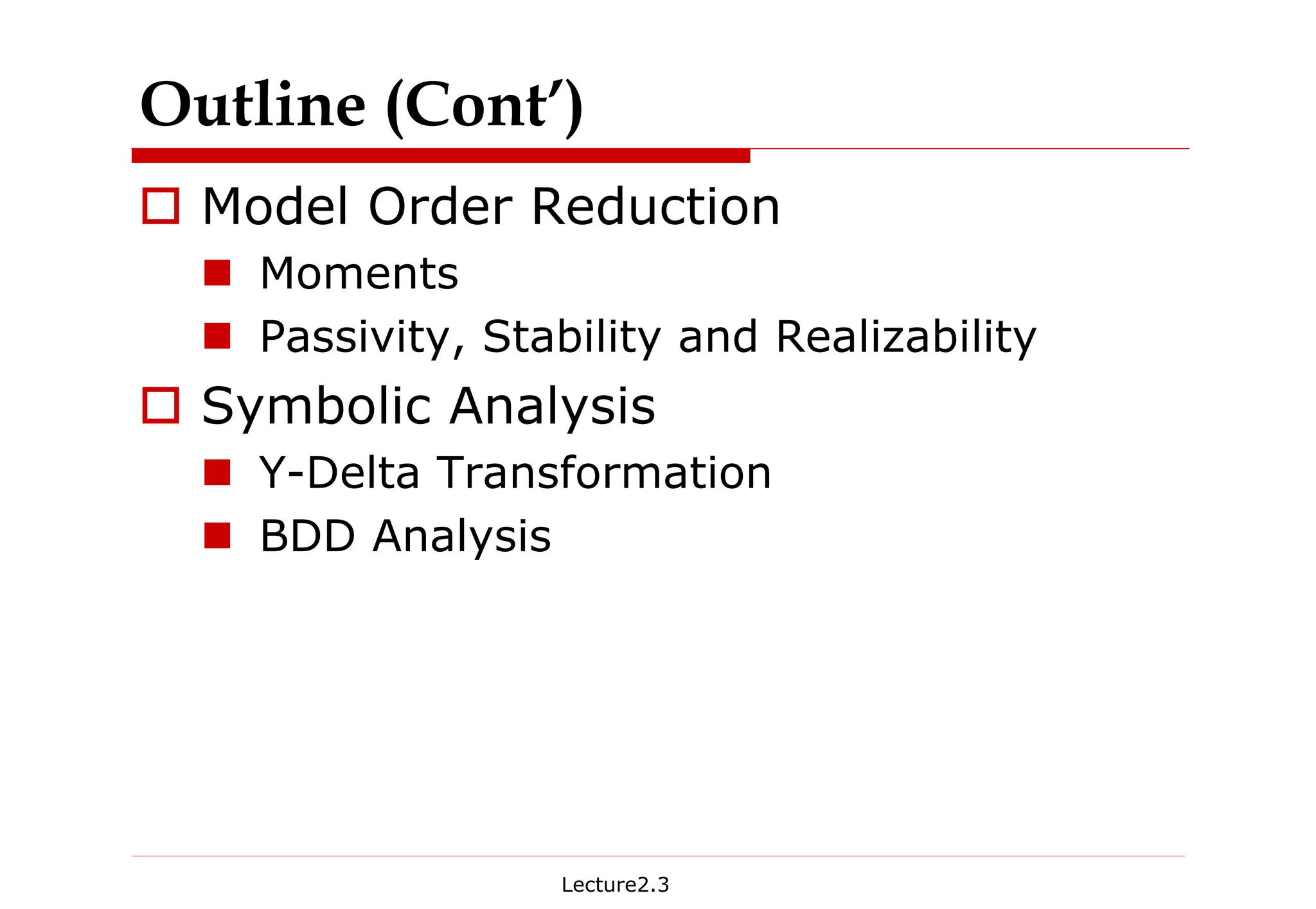
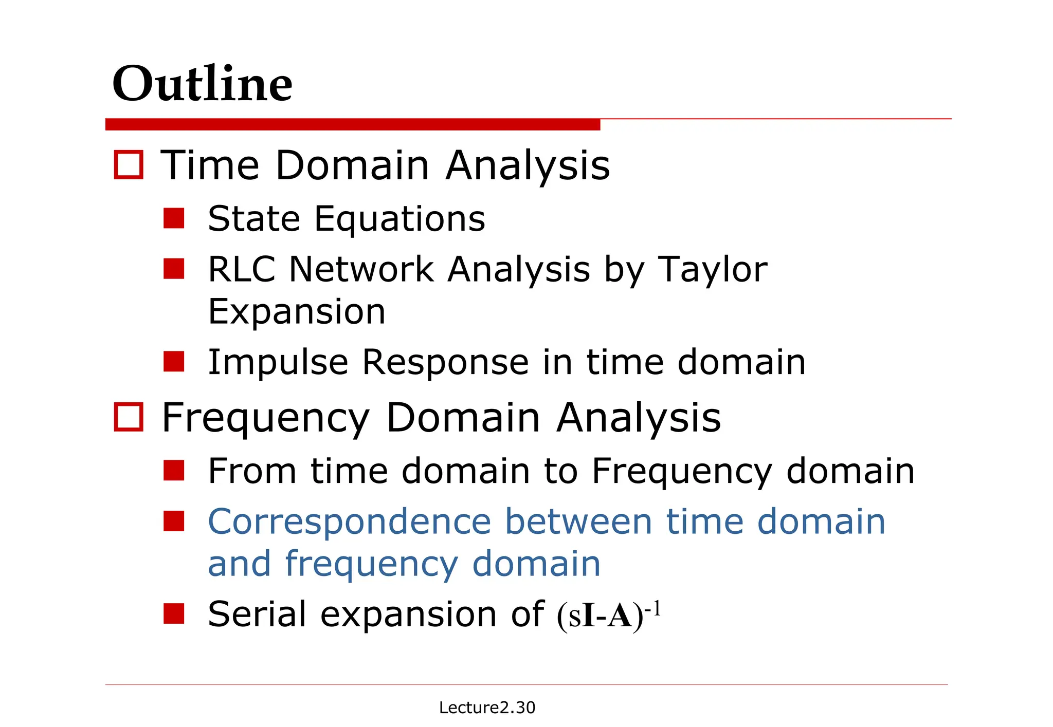
Correspondence between time
domain and frequency domain
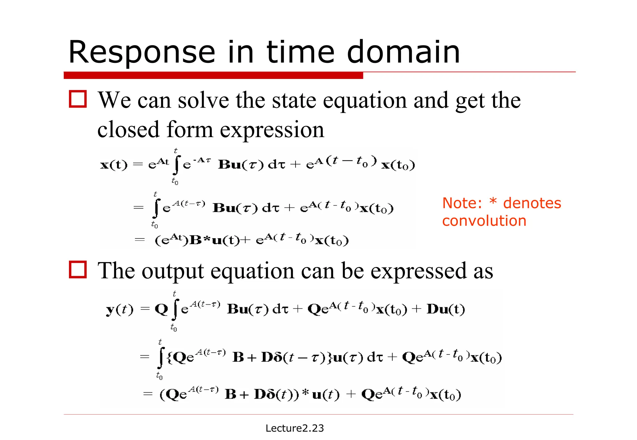
† We can derive the time domain solutions of the
network from the s domain solutions by inverse
Laplace Transformation of the s domain solutions.
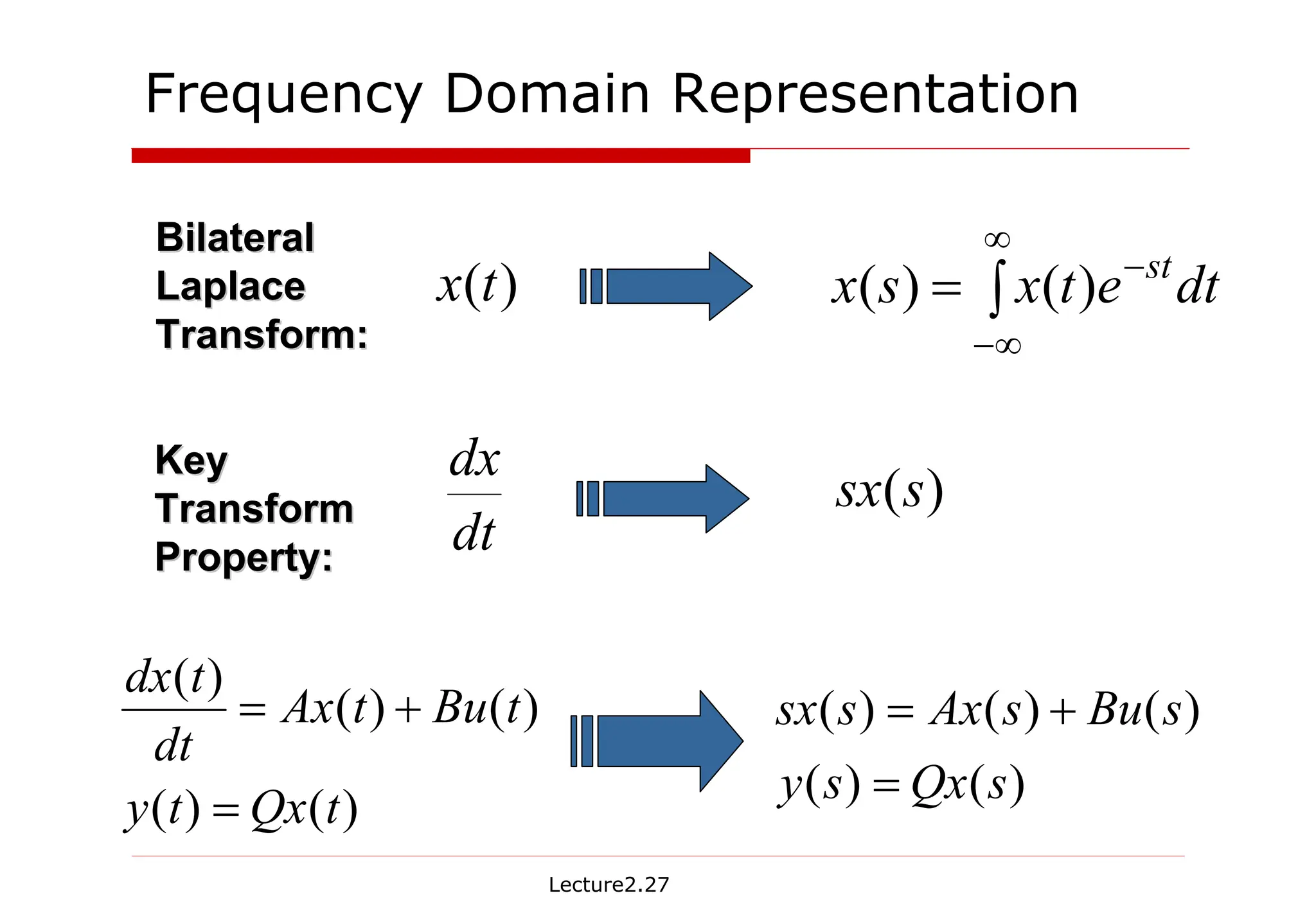
State Equations
in S domain
State Equations
in time Domain
Inverse Laplace
Transform
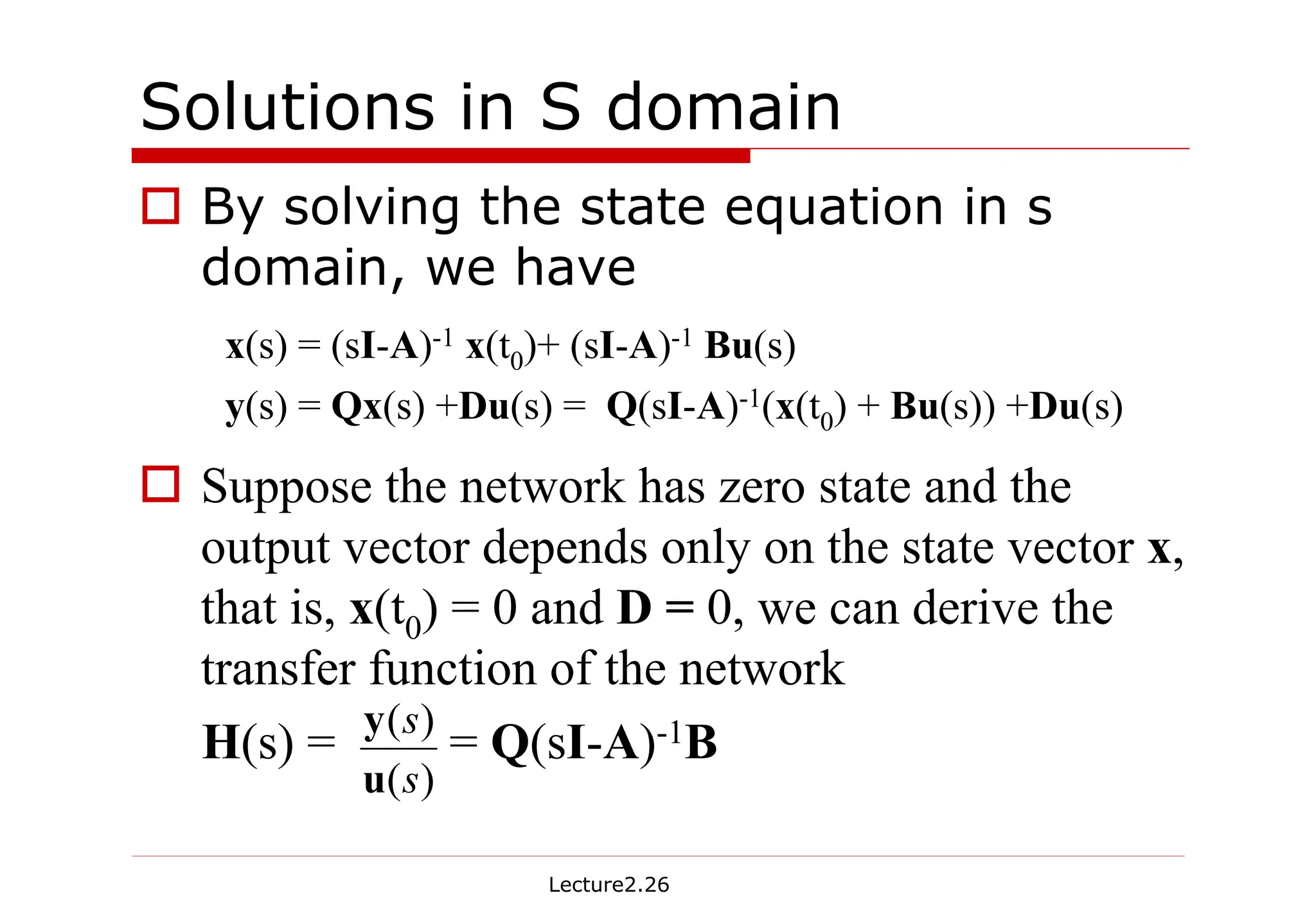
sx(s) – x(t0)= Ax(s) +Bu(s)
y(s) = Qx(s) +Du(s)
x(t) = L-1[(sI-A)-1x(t0) + (sI-A)-1 Bu(s)]
= L-1[(sI-A)-1]x(t0) + L-1[(sI-A)-1]B*u(t)
y(t) = L-1[Q(sI-A)-1(x(t0) + Bu(s)) +Du(s)]
= Q L-1[(sI-A)-1] x(t0) + {QL-1 [(sI-A)-1]B +Dδ(t)}* u(s)

32. Lecture2.32
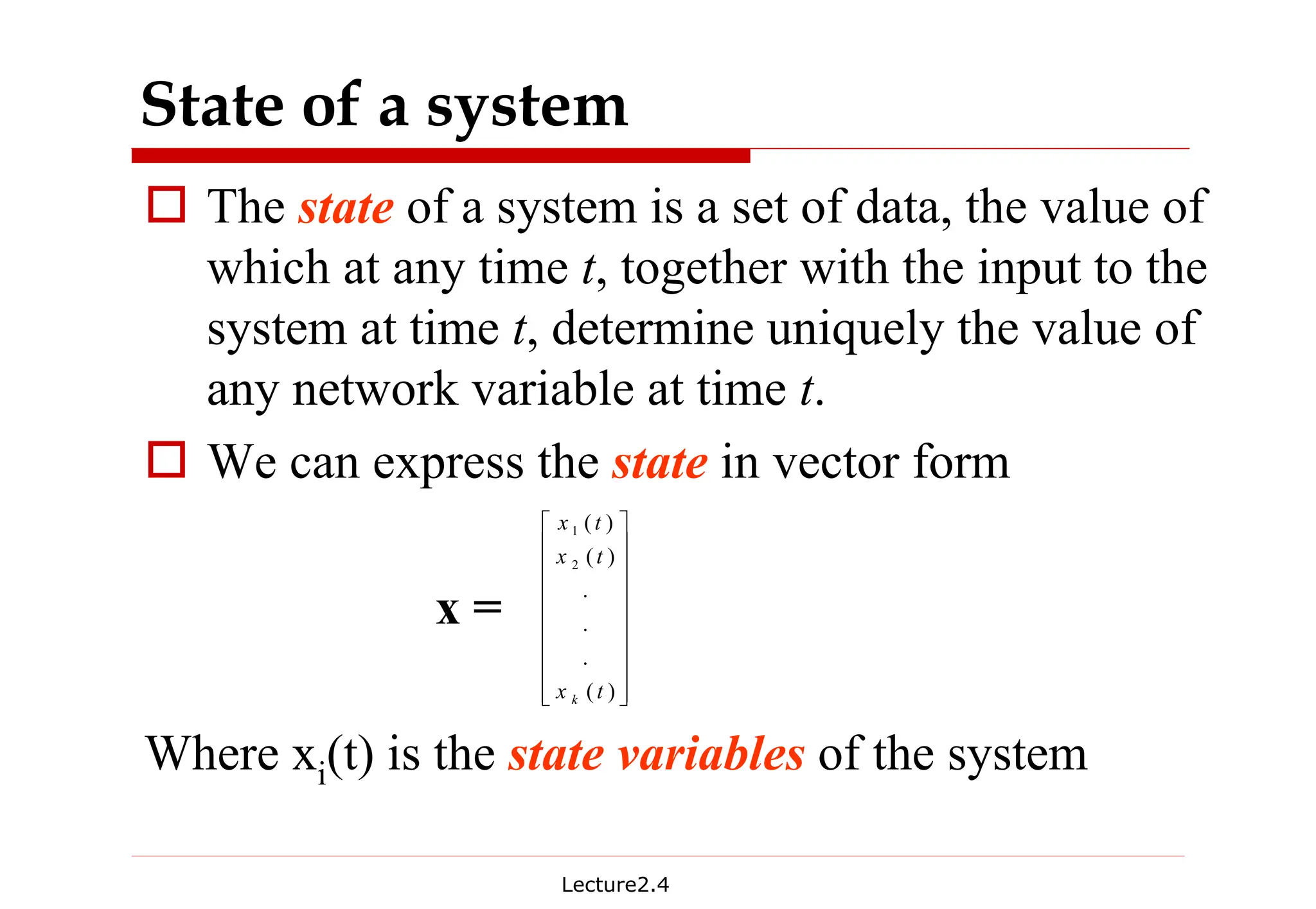
Correspondence between time
domain and frequency domain
† (sI-A)-1 eAt
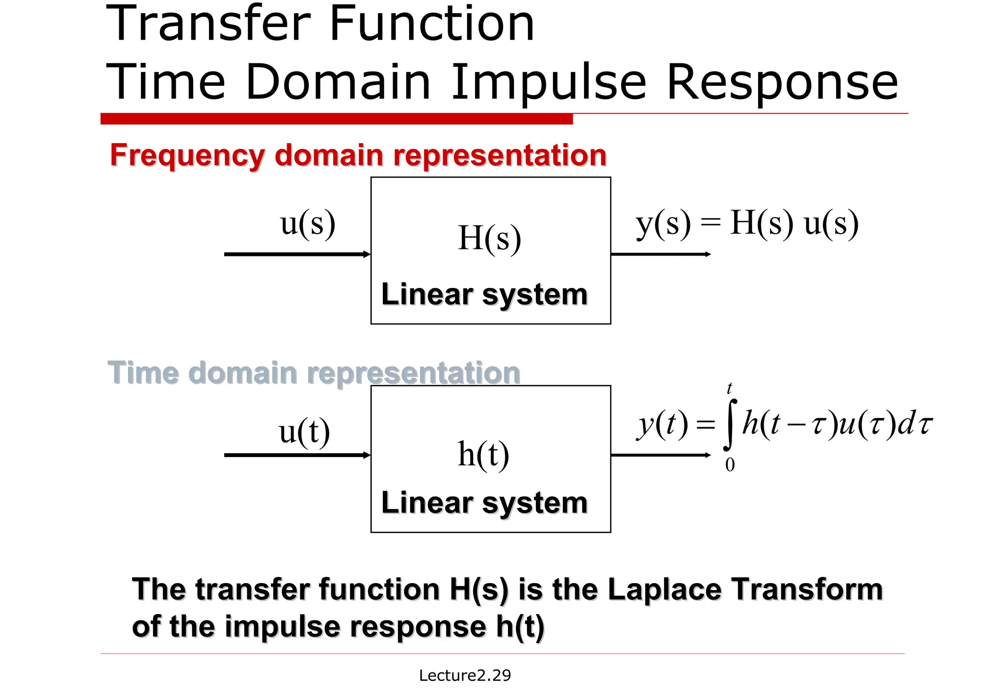
† multiplication of u(s) in s domain corresponds
to the convolution in time domain
Solution from
time domain
analysis
Solution by
inverse Laplace
transform
x(t) = L-1[(sI-A)-1x(t0) + (sI-A)-1 Bu(s)]
= L-1[(sI-A)-1]x(t0) + L-1[(sI-A)-1]B*u(t)
y(t) = L-1[Q(sI-A)-1(x(t0) + Bu(s)) +Du(s)]
= Q L-1[(sI-A)-1] x(t0) + {QL-1 [(sI-A)-1]B +Dδ(t)}* u(s)

33. Lecture2.33
Outline
† Time Domain Analysis
„ State Equations
„ RLC Network Analysis by Taylor
Expansion
„ Impulse Response in time domain
† Frequency Domain Analysis
„ From time domain to Frequency domain
„ Correspondence between time domain
and frequency domain
„ Serial expansion of (sI-A)-1

34. Lecture2.34
Serial expansion of (sI-A)-1
† When sÆ0 we can write (sI-A)-1 as
† Thus, the transfer function can be written as
† When sÆ∞ we can write (sI-A)-1 as
† The transfer function can be written as
(sI-A)-1 = -A-1(I – sA-1) = -A-1(I + sA-1 + s2A-2 + … + skA-k + …)
H(s) = Q(sI-A)-1B = -QA-1(I + sA-1 + s2A-2 + … + skA-k + …)B
(sI-A)-1 = s-1(I – s-1A)-1 = s-1(I + s-1A + s-2A2 + … + s-kAk + …)
H(s) = Q(sI-A)-1B = s-1(I + s-1A + s-2A2 + … + s-kAk + …)B

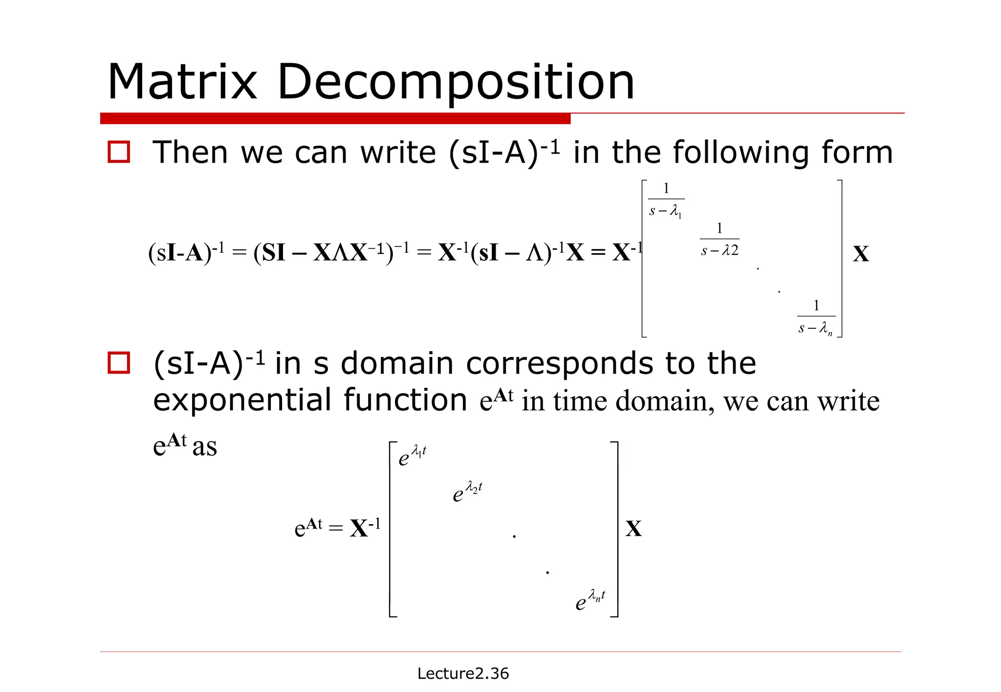
35. Lecture2.35
†Assume A has non-degenerate eigenvalues
and corresponding linearly
independent eigenvectors , then A
can be decomposed as
where and
Matrix Decomposition
1
−
ΧΛΧ
=
A
k
Χ
Χ
Χ ,...,
, 2
1
k
λ
λ
λ ,...,
, 2
1












=
Λ
k
λ
λ
λ
L
L
M
O
L
M
M
L
L
0
0
0
0
2
1
[ ]
k
Χ
Χ
Χ
=
Χ ,...,
, 2
1

36. Lecture2.36
Matrix Decomposition
† Then we can write (sI-A)-1 in the following form
† (sI-A)-1 in s domain corresponds to the
exponential function eAt in time domain, we can write
eAt as
(sI-A)-1 = (SI – XΛX-1)-1 = X-1(sI – Λ)-1X = X-1






















−
−
−
n
s
s
s
λ
λ
λ
1
.
.
2
1
1
1
X
eAt = X-1
















t
t
t
n
e
e
e
λ
λ
λ
.
.
2
1
X