The document discusses transmission line theory, focusing on the distinctions between lumped and distributed circuits, the derivation of time domain equations, and their solutions using finite-difference time-domain (FDTD) methods. It also covers numerical convolution methods for simulating transmission lines and addresses both lossless and lossy cases. References are provided for further reading on the topic.

1. September 17, 2024 1
CSE 245: Computer Aided Circuit
Simulation and Verification
Fall 2004, Nov
Transmission Line Simulation

2. September 17, 2024 2
Outline
 Transmission Line Equations
 FDTD Solution of The Transmission
Line Equations
 Convolution Simulation of
Transmission Lines

3. September 17, 2024 3
Lumped V.S. Distributed Circuits
 Lumped circuit:
 In circuit theory, we assume the physical dimensions of
a circuit element are much smaller than the electrical
wavelength.
 Resistor, Capacitor, Inductor, Independent and
dependent sources are lumped circuit elements
 The voltages and currents in such a circuit are functions
of time only.
 Distributed Circuit:
 In a distributed circuit, for example in a transmission
line circuit. The size of the transmission line may be a
considerable fraction of a wavelength, or many
wavelengths.
 Thus a transmission line can’t be modeled as a lumped
circuit element. It should be modeled as a distributed
parameter network, where voltages and currents are
functions of position as well as time

4. September 17, 2024 4
Transmission Line Circuit Model
( , )
( , ) ( , ) ( , ) 0,
( , ) ( , ) ( , )
( , )
0,
( , ) ( , )
( , )
I x t
V x t R xI x t L x V x x t
t
V x x t V x t I x t
RI x t L
x t
x
V x t I x t
RI x t L
x t

       

  
  
 
  
 
 
 
From KVL we can derive:

5. September 17, 2024 5
Transmission Line Equations
 Similarly, by using KCL we can derive:
 Put them together, we have the time
domain transmission line equations:
 C – Capacitance per unit length
 L – Inductance per unit length
 R – Resistance per unit length
 G – Conductance per unit length
( , ) ( , )
( , )
I x t V x t
GV x t C
x t
 
 
 
( , ) ( , )
( , )
( , ) ( , )
( , )
V x t I x t
RI x t L
x t
I x t V x t
GV x t C
x t
 
 
 
 
 
 

6. September 17, 2024 6
Taylor Series

7. September 17, 2024 7
Central Difference Approximation
 Subtracting:
 Similarly we could derive:
 Note that second-order accuracy is obtained at (x,t) by
differencing two discrete points centered by (x,t).
Hence, this is called a central difference approximation.

8. September 17, 2024 8
FDTD Solution of the Tx-Line Equations (Lossless)
 Lossless Transmission Line Equations (R=G=0):
 Let
 We have the Discrete Transmission Line Equations:
 Observing the above equations, we can write a recursive
relationship to compute Vi
n+1/2
given the previous values of V
and I:
 Similarly:
( , )
n
i i n
f f x t


9. September 17, 2024 9
FDTD Solution of the Tx-Line Equations (lossy)
 Lossy Transmission Line Equations:
 Discrete Transmission Line Equations:
 Averaging loss terms in
time for second order accuracy:
( , ) ( , )
( , )
( , ) ( , )
( , )
I x t V x t
GV x t C
x t
V x t I x t
RI x t L
x t
 
 
 
 
 
 

10. September 17, 2024 10
Summary: FDTD Solution of the Tx-Line Equations
 FDTD Summary:
 Line axis x is discretized in Δx increments or spatial
cells, the time variable t is discretized in Δt
increments or temporal cells.
 The derivatives in the Tx-Line Equations are
approximated by central differences.
 Given the initial condition of V and I along the entire
line length, V and I can be time advanced.
 The accuracy of the solution depends on having
sufficiently small spatial (Δx) and temporal (Δt) cell
sizes

11. September 17, 2024 11
Transmission Line Equations In Frequency Domain
 Time domain Transmission Line Equations:
 For the transmission line shown above, l is the length of the
line. The boundary conditions for the transmission line
equations are:
 By taking Laplace transformation of the time domain transmission line
equations we get the frequency domain equations:
)
(t
x ( )
x s
dt
dx
)
(s
sx
( , )
( ) ( , )
( , )
( ) ( , )
V x s
R sL I x s
x
I x s
G sC V x s
x

 


 

( , ) ( , )
( , )
( , ) ( , )
( , )
V x t I x t
RI x t L
x t
I x t V x t
GV x t C
x t
 
 
 
 
 
 

12. September 17, 2024 12
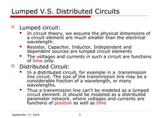
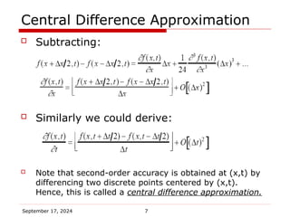
Convolution Simulation of Transmission Lines
 From the frequency domain Tx-line equations, we could obtain (for
mathematical details, see [3])
 Inverse Laplace Transformation to time domain, we get:
 where
 At each time point, the integration of a circuit with RLGC-lines will
involve the convolution of (1) and (2) for each line, where the v1, v2, i1
and i2 at that time point are the only unknown variables to be
determined. Then the circuit equations are composed of KCL equations
for each node of the circuit and equations (1) and (2)
* denotes convolution
(1)
(2)
( )
v t
( )
V s
( )
y t
( )
Y s
( )* ( )
y t v t
( ) ( )
Y s V s

13. September 17, 2024 13
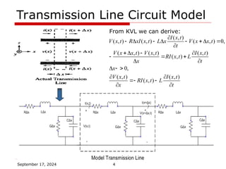
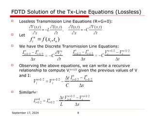
Numerical Convolution
 Convolution is the most computational demanding part.
 Given two functions x(t) and h(t), the convolution integral to be
calculated is the following:
 Generalized Backward Euler Methods:
 Assume x(t) is piecewise constant:
x(t)≈xi+1, t (ti,ti+1]
 Using (4), the integral in (3) is split up into a sum of integrals over
the piecewise constant regions and expressed as:
 Equation (5) is evaluated by parts and algebraically manipulated to
arrive at the following:

0
( , ) ( )
t
E h t h d
 


0
( ) ( )* ( ) ( ) ( )
t
y t x t h t x h t d
  
  
 (3)
(4)
1
1
1
0
( ) ( )
i
i
t
n
n i n
i t
y t x h t d
 




 
 
1
1 1
1
( ) ( , ) [ ( , ) ( , )]
n
n n n n i n i n i
i
y t x E h t t x E h t t E h t t

 

     


14. September 17, 2024 14
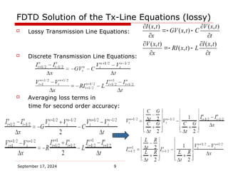
Numerical Convolution
 If we assume x(t)≈xi, t [ti,ti+1), a generalized forward
Euler method could be derived.
 Similarly, by assuming x(t) is piecewise linear we could
derive the generalized trapezoidal convolution method.
For details, see [3]


15. September 17, 2024 15
References:
 [1] Finite-difference, time-domain analysis of lossy transmis
sion lines, Roden, J.A. Paul, C.R. Smith, W.T. Gedney, S.
D. IEEE Transactions on Electromagnetic Compatibility, Feb
1996
 [2] EE669 class notes, Stephen Gedney, University of Kentuc
ky
 [3] Algorithms for the Transient Simulation of Lossy Intercon
nect. J. S. Roychowdhury, A.R. Newton, D.O. Pederson. IEEE
Transactions on Computer-Aided Design of Integrated Circuit
s and Systems. Vol. 13, No. 1. Jan 1994
 [4] Transient Simulation of Lossy Interconnects Based on th
e Recursive Convolution Formulation, S. Lin and E.S. Kuh, IE
EE Transactions on Circuits and Systems – I, Vol. 39, No. 11,
Nov 1992