Dynamic Pricing andRevenue ManagementIEOR 4601 Spring .docx

Dynamic Pricing and
Revenue Management
IEOR 4601 Spring 2013
Professor Guillermo Gallego
Class: Monday and Wednesday 11:40-12:55pm
Office Hours: Wednesdays 3:30-4:30pm
Office Location: 820 CEPSR
E-mail: [email protected]
Why Study Dynamic Pricing and Revenue
Management?
¡� Revenue Management had its origins in the
airline industry and is one of the most
successful applications of Operations
Research to decision making
¡� Pricing and capacity allocation decisions
directly impact the bottom line
¡� Pricing transparency and competition make

pricing and capacity allocation decisions
more difficult and more important
Applications of Dynamic Pricing and
Revenue Management
¡� Capacity allocation of limited, perishable,
resources to different fare classes
l� Airlines, hotels, car rentals, cruises, travel packages, tickets
for events
¡� Design and pricing of products
l� Fare restrictions and pricing
l� Consumption and fulfillment options
l� Upgrades, downgrades and upsells
¡� Pricing under competition
l� Electronic-commerce
Objectives of this course
¡� Understand the critical tradeoffs and
decisions in Revenue Management

¡� Learn how to
l� Monitor and control product availability for single and
multiple resources
l� Overbook limited resources when customers
shows are random
l� Use upgrades, upsells and real options to improve revenues
l� Price under competition
l� Improve on the current practice of Revenue
Management
“Physics should be explained as simply as possible, but no
simpler.”
Albert Einstein
Professor Gal ego’s experience and
background on subject
¡� Author of seminal papers on dynamic
pricing and revenue management
¡� Winner of several prices from academia
and industry related to work on Revenue
Management

¡� Consultant for airlines and RM solution
providers
¡� Consultant for other users of Revenue
Management
Readings
¡� Class Notes
l� I will provide with notes of the different topic we cover in
class
¡� Textbook
l� R.L. Phillips, Pricing and Revenue
Optimization, Stanford University Press,
2005, ISBN 0-8047-4698-2.
¡� References
l� K.T. Talluri and G.J. Van Ryzin, The Theory and Practice of
Revenue Management,
Springer, 2005, ISBN 0-387-24376-3.
l� Assigned papers
Prerequisites and Grading

¡� Prerequisites
l� Probability and Statistics at the level of IEOR
4150
l� Deterministic Models at the level of IEOR 4003
¡� Corequisites: Stochastic Models IEOR 4106
¡� Grading
l� Assignments
20%
l� Midterm
35%
l� Final
45%
Introduction to Revenue Management
¡� Revenue Management refers to the
strategy and tactics used by perishable
capacity providers to allocate capacity to
different fare classes or market segments

to maximize expected revenues. (See
Chapter 6 in Phillips.)
¡� RM is often practice when
l� Sellers have fixed stock of perishable capacity l�
Customers book capacity prior to usage
l� Seller offers a sets of fare classes
l� Seller can change the availability of fare
classes
History of Revenue Management
¡� Prior to 1978 the Airline Industry was
heavily regulated
¡� In the early 80’s the industry was
deregulated to encourage new entrants
¡� Low-cost carriers such as People Express
started encroaching into key markets of
large carriers
¡� American Airline dilemma:
l� Match fares and lose money

l� Keep fares and lose customers
AA’s Response to People Express
¡� Ultimate Super Saver Discount Fare
l� Same fare as People Express
l� Passenger must buy at least two weeks
prior to departure
l� Stay at his destination over a Saturday
night
¡� AA restricted the number of
discount seats sold on each flight to
save seats for full-fare passengers
Rational and Impact of Strategy
¡� Product Design
l� Imposing restrictions that appealed to the
leisure segment without cannibalizing the
business segment
¡� Capacity Allocation
l� Carefully control capacity to maximize

revenues
¡� Strategy started in January 85
l� PE was struggling by March
l� PE was at the verge of bankruptcy by August
Post-mortem
¡� People Express was bought by
Texas Air for 10% of the market
value it had enjoyed a year before
¡� “We had great people, tremendous
value, terrific growth. We did a lot
of things right. But we didn’t get
our hands around the yield
management and automation
issues.” Donald Burr CEO of PE
RM: The System Context
¡� AA was based on a computerized
reservation system (CRS) called Sabre

developed in 1963. This system:
l� Replaced index cards to manage reservations
l� Sabre is also a GDS (global distribution
system) that allowed AA to distribute its
products and fares globally
¡� Other GDSs: Amadeus, Galileo, Worldspan.
RM Constraints Imposed by Systems
¡� AA’s used Sabre’s Computerized
Reservation System as the backbone to
Revenue Management
l� The reservation system served as a repository of all the
bookings that have been accepted for
future flights
l� The CRS also contains the controls that specify how many
bookings from different fare classes
the airline will accept on future flights
¡� Remember: RM systems were developed
in the context of existing CRSs.

Levels of Revenue Management
¡� Strategic:
l� Market segmentation (leisure vs business)
l� Product design (restrictions, fares, options) l� Pricing
(Static vs. Dynamic)
¡� Tactical:
l� Calculate and updated booking limits
¡� Booking Control:
l� Determine which booking to accept and which
to reject based on booking limits
Strategic Revenue Management
¡� Design low fares to increase sales without
cannibalizing full fare demand
l� Time of Purchase Restrictions
¡� Advance purchase requirements
l� Traveling Restrictions
¡� Saturday night stays
l� High cancellation and change penalties

¡� Other opportunities
l� Contingent options on capacity
l� Flexible and callable products
Tactical Revenue Management
¡� Resources
l� Units of capacity
¡� Seats on a flight
¡� Hotel capacity for a specific night
¡� Products
l� What consumers seek to purchase
¡� May involve one or more resources
¡� Fares
l� A combination of a price and a set of
restrictions
Tactical Definition of RM
¡� A supplier controls a set of resources with
fixed and perishable capacity, a portfolio

of products consisting of combinations of
one or more of the resources, and a set of
fare classes associated with each of the
products. The tactical revenue
management problem is to chose which
fare classes should be open and which
closed for sale at each moment to
maximize total revenue.
Components of Tactical RM
¡� Capacity Allocation
l� How many customers from different
fare classes should be allowed to book?
¡� Network Management
l� How should bookings be managed
across a network of resources?
¡� Overbooking
l� How many total bookings should be

accepted for a product when there are
cancellations and show uncertainty?
Booking Controls
¡� Limits on bookings for different fare
classes:
l� Example: An airline receives a B-class
request for 3 seats departing in two
weeks. The current B-class booking
limit is two seats. As a result, the
request is rejected
Booking Limits
¡� Nesting Controls:
l� Label the fare classes so that 1 is the highest fare class and
n is the lowest fare class. For any i let bi
denote the nested booking limit for class i.
b 1 ≥ b 2 ≥�≥ bn
l� Protection Levels:
y
�

i = b − b
, i
i
= ,
1 2, n −1
1
1
+
l� Updates: If x units are sold in a transaction b
�
i ← max( bi − x
),
0
,
i = ,
1 2, n −1
Nested Booking Limits (Example)

Booking Limits
Protection Levels
Requests
1
2
3
4
5
1
2
3
4
5 Seats
Class
Action
1
100

73
12
4
0
27
88
96
100
100
2
5 Reject
2
100
73
12
4
0
27

88
96
100
100
5
2 Accept
3
95
68
7
0
0
27
88
95
95
95

1
2 Accept
4
94
67
6
0
0
27
88
94
94
94
1
4 Reject
5
94

67
6
0
0
27
88
94
94
94
3
3 Accept
6
91
64
3
0
0
27

88
91
91
91
4
3 Reject
7
91
64
3
0
0
27
88
91
91
91

2
3 Accept
8
89
62
1
0
0
27
88
89
89
89
Is RM successful?
¡� By most measures (revenues relative to
resources) it has been a success at most
major airline, hotel, rental car companies.

l� Why have major airlines have been losing
money?
¡� Costs are 25-30% higher per mile, so even though larger
carriers bring in about 25% more revenue
per mile the cost disadvantage is overwhelming
l� What can be done?
¡� Cost costs
¡� Improve RM systems
l� Big move from independent to dependent demand models
RM and Price Discrimination
¡� Price discrimination exists when sales of identical goods or
services are transacted at different
prices from the same provider.
¡� A feature of monopolistic or oligopolistic markets where
market power can be exercised.
¡� Requires market segmentation and means to discourage
discount customers becoming resellers.
l�
This is achieved by fences to keep segments separate.
¡� Price discrimination is more common in services where
resale is not possible.

¡� Price discrimination can also be seen when the requirement
of identical goods is relaxed.
l�
Premium products have price differential not explained by
production costs.
Taxonomies of Price Discrimination
¡� First degree: requires selling at maximum willingness to pay
¡� Second degree: quantity discounts (sellers not able to
differentiate consumer types)
¡� Third degree: Prices vary by attributes (e.g., senior
discounts)
¡� Fourth degree: Prices are the same but costs are different
(reverse discrimination)
¡� Alternative taxonomy:
l�
Complete discrimination (like first degree)
l�
Direct discrimination: seller conditions price on some attribute
(like third degree)
l�

Indirect discrimination: the seller relies on some proxy such as
quantity discounts (like second degree)
RM and Price Discrimination
¡� Differentiating by time-of-purchase and imposing traveling
restrictions like Saturday night stays is a
form of second degree or indirect discrimination.
¡� Selling premium seats is another form of second degree or
indirect discrimination.
l� Eg., uncomfortable second class seats on trains to entice
wealthier people to purchase first class
seats.
l� Advance seat selection, mileage accrual, use of lounge, and
priority boarding may be forms of second
and/or fourth degree discrimination.
Other Examples of Price Discrimination
¡� Retail price discrimination is in violation of the Robinson-
Patman Act (1936)
¡� Coupons
¡� Segmentation by age group and student status
¡� Discounts for members of certain occupations
¡� Employee discounts
¡� Retail incentives (rebates, seasonal discounts, quantity
discounts)

¡� Gender based examples
¡� College financial aid
¡� User-controlled price discrimination
¡� See http://en.wikipedia.org/wiki/Price_discrimination Static
and Dynamic Pricing
¡� Pricing is studied by people in Economics
and Marketing
¡� Economist look at equilibrium prices
¡� Marketing focuses on demand estimation
¡� We focus on more tactical aspects of
pricing
l� Customer arrival rates
l� Capacity constraints
l� And increasingly on choice models and
competition
Static Pricing
¡� d(p) demand at p
¡� z unit cost or dual of capacity constraint

¡� r(p,z) = (p-z)d(p) profit function
¡� Find p to maximize r(p,z)
¡� Is there a finite maximizer p(z)?
¡� Is p(z) monotone?
¡� Is r(z) = r(p(z),z) monotone? Convex?
¡� Multiple market segments with limited
price menus
Dynamic Pricing
¡� Finite sales horizon
¡� Customers arrive stochastically over time
¡� State (t,x)
l� t time-to-go
l� x remaining inventory
¡� What price p(t,x) should be charged at
state (t,x)?
¡� Are there simple and effective pricing
heuristics?

¡� What about strategic customers?
¡� What about competition?
Topics to be Covered
¡� Single Resource RM
l� Independent Demands
¡� Dynamic Programming, Bounds and Heuristics
l� Dependent Demands based on choice models
¡� Static and Dynamic Pricing
¡� Network RM
l� Independent Demands, Choice Models
¡� Overbooking
¡� Service Engineering
l� Design and pricing of service features
Useful Techniques you wil Learn
¡� Dynamic Programming (DP)
l� Tool for sequential decision making
l� Optimal Control (continuous time DP)

¡� Approximate Dynamic Programming
l� Tool to approximate DPs
¡� Bounds and Heuristics Techniques
¡� Choice Modeling
¡� Game Theory
Single Resource Revenue Management with Independent
Demands
c
Guillermo Gallego
Updated Spring 2013
Abstract
Providers of fixed perishable capacity, such as airline seats and
hotel rooms use price discrimination
to improve revenues; in practice, this discrimination is typically
achieved by imposing booking and usage
restrictions or including ancillary services such as mileage
accrual and luggage handling, to sell the same
capacity to different customers at different prices. We will
assume that the set of fare classes (a menu

of prices, restrictions and ancillary services) is given, and that
the capacity provider’s goal is to allocate
capacity among the different fare classes to maximize expected
revenues. The problem of designing and
pricing fare classes is treated in a separate chapter. We analyze
the two fare class problem under the
assumption that the lower fare class books first. We use
marginal analysis to informally derive
Littlewood’s
rule and then show that Littlewood’s rule is in fact optimal.
Spill rates, spill penalties and callable
products are discussed next. A dynamic programming
formulation for the multiple fare class problem is
then introduced under the assumption that lower fare classes
book first. Commonly used heuristics as well
as bounds on the value function are presented. Dynamic models
that explicitly take time into account,
allow for more general fare arrival patterns and for randomness
in the size of the requests. We compare
the performance of static and dynamic policies and find that
dynamic policies have a real advantage when
the fare arrivals patterns are not low-to-high. We finalize the
chapter with a model where fare classes are

not allowed to reopen after they are closed for the first time.
1
Introduction
This chapter considers the simplest and best known revenue
management problem, the single resource,
inde-
pendent demand problem. We assume that the capacity provider
is trying to maximize the expected
revenues
from a sunk investment in c units of capacity. We assume that
capacity is sold through a reservation
system
and that capacity cannot be modified or replenished during the
booking horizon. We also assume that
unsold
capacity has no salvage value. Later we will see that the zero
salvage value assumption is made without
loss
of generality as any problem with positive salvage value can be
transformed into a problem with zero
salvage
value. We assume that the set of fare classes (a menu of prices
and restrictions) is given, and that the
demands

for the different fare classes are statistically independent. In
particular, we assume that if a customer finds
his
preferred fare class closed, he will leave the system without
purchasing. This assumption holds
approximately
if the difference in fares is large so that demands are decoupled
or if customers can find alternative
sources
of capacity for their preferred fare class. In some cases,
however, part of the demand may be recaptured
by
other available fare classes. In such cases, the independent
demand assumption is too strong and needs to
be
relaxed. We address this issue in a separate chapter where we
discussed demand models based on
discrete
choice theory.
In this chapter, we present a variety of models that have been
developed in industry and in academia.
There has been a preference in industry for models that suppress
the time dimension and assume that the
arrival pattern of the fare classes is low-to-high. We call these
class of models static to distinguish them

from the dynamic models, favored by academics, that model
time explicitly. Both models have advantages
and disadvantages as we will soon see. Static models are
relatively easy to understand. Also, good
heuristics
1
were developed before optimal solutions based on dynamic
programming were discovered. Bringing in
the
time dimension helps deal with more general fare arrival
patterns, but specifying the model requires a
more
detailed estimation of demand. This Chapter starts with a
review of the two fare class problem in §2
where we
present a heuristic derivation of Littlewood’s rule via marginal
analysis. Littlewood’s rule is formally
derived
in §2.3 where a formal DP for the two fare class problem is
presented. The dynamic program for multiple
fare
classes is presented in §3. Commonly used heuristics are
presented in §4 and bounds on the optimal
expected
revenue are presented in §5. The dynamic model is presented in
§6, for the Poisson case and for the

compound
Poisson case in §7, where each request is for a random demand
size. In §8, we restrict fares so that they
cannot
be opened once they are closed.
2
Two Fare Classes: Marginal Analysis
The product can be sold either at the full-fare p1 or at a
discounted-fare p2 < p1. The discounted-fare
typically
has advance purchasing and usage restrictions. Let D1 and D2
denote respectively the random demand for
the two fare classes for a specific instance of the problem, e.g.,
for a specific flight for an airline or a
specific
night for a hotel.
We assume that all booked customers will actually travel. This
avoids the need to overbook capacity and
allow us to focus on the problem of allocating capacity between
the two fares. We will discuss how to
deal
with pre-travel cancellations and day-of-travel no shows in a
separate chapter on overbooking models.

Fare class arrival order is an important part of the model. We
assume what is commonly known as the
low-to-high fare class arrival order, which implies that demand
for the discounted fare book earlier than
for
full-fare. This arrival pattern holds approximately in practice,
and it is encouraged by advance purchase
restrictions imposed on lower fare classes. Notice that this is a
worst case arrival pattern. Indeed, if full-
fare
class customers arrived first then we would accept them up to
capacity and use residual capacity, if any,
to
satisfy demand from the discounted-fare class. We will relax the
low-to-high fare order arrival
assumption
after we solve the multi-fare problem via dynamic
programming.
Under the low-to-high arrival pattern, discount-fare customers
may exhaust capacity, say c, unless part
of it is protected for later-booking by full-fare customers.
Consequently, booking limits (known as
discount
authorizations) are placed on the discount sales. Suppose we
protect y ∈ {0, 1, . . . , c} units of capacity
for

the full-fare demand, D1, before observing the actual demand
for the discount-fare, D2. This results in a
booking limit c − y on the discounted-fare, so sales at the
discounted-fare class are given by min(c − y,
D2).
The remaining capacity is equal to c − min(c − y, D2) = max(y,
c − D2) and it is all made available to the
full-fare class. Consequently, sales at the full fare equal
min(max(y, c − D2), D1). The total expected
revenue
is
W (y, c) = p2E min(c − y, D2) + p1E min(max(y, c − D2), D1)
and the goal is to find a protection level y that maximizes W (y,
c). The extreme strategies y = 0 and y = c
correspond, respectively, to the case where no capacity is
protected and all of the capacity is protected.
We
will later come back and discuss when these extreme strategies
are optimal. In most cases, however, an
intermediate strategy is optimal.
The fare ratio r = p2/p1 plays an important role in determining
optimal protection levels. If the ratio is

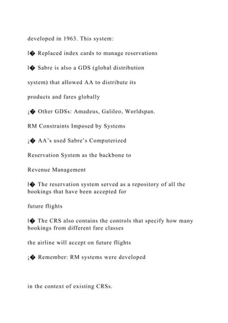
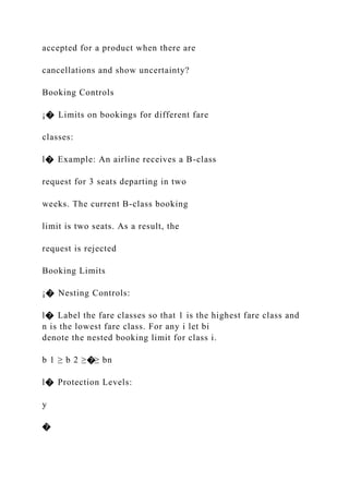
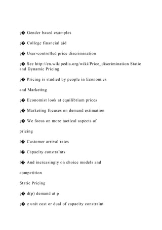
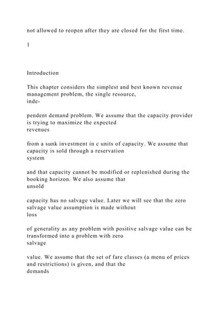
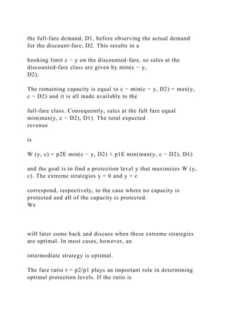
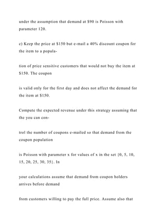
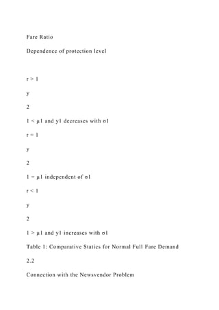
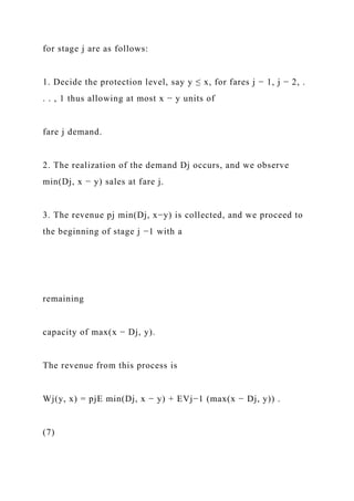
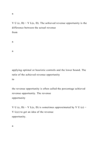
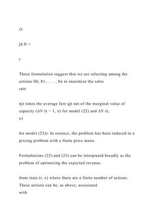
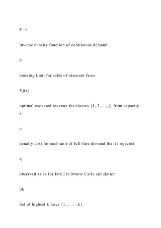
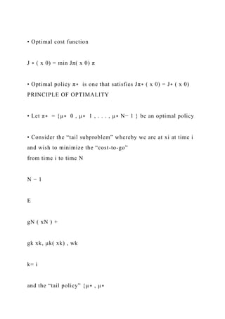
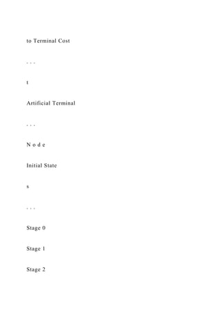
very small then we would be inclined to protect more capacity
for the full-fare demand. If the ratio is
close
to one, we would be inclined to accept nearly all discount-fare
requests since we can get almost the same
revenue, per unit of capacity, without risk. The distribution of
full-fare demand is also important in
deciding
how many units to protect for that fare. If, P (D1 ≥ c) is very
large, then it makes sense to protect the
entire
capacity for full-fare sales as it is likely that the provider can
sell all of the capacity at the full-fare.
However,
if P (D1 ≥ c) is very low then it is unlikely that all the capacity
can be sold at the full-fare, so fewer units
should be protected. It turns out that the demand distribution of
the discount-fare D2 has no influence on
the
optimal protection level under our assumption that D2 and D1
are independent. A formula for the optimal
protection level, involving only P (D1 ≥ y) and r, was first
proposed by Littlewood [14] in 1972. His
arguments
were not formal; however, they were later justified by Bhatia
and Prakesh [1] in 1973, and Richter [17]
in 1982.

2
One can obtain Littlewood’s formula intuitively by using
marginal analysis. The advantage of marginal
analysis is that it allows us to quickly derive the solution for the
two fare class problem. The marginal
analysis
argument goes as follows: Suppose we have y > 0 units of
capacity, and that we receive a request for the
discounted-fare. Consider the marginal revenue associated with
accepting and rejecting this request. If we
accept, we obtain p2. If we close down the discount-fare then
we will be able to sell the yth unit at p1
only
if the full-fare demand D1 is at least as large as y, so it is
intuitively optimal to reject the discount fare if
p1P (D1 ≥ y) > p2. This suggests that an optimal protection
level y1 should be given by:
y1 = max{y ∈ N : P (D1 ≥ y) > r},
(1)
where N = {0, 1, . . . , } is the set of non-negative integers.
Equation (1) is known as Littlewood’s rule.
Example 1. Suppose D1 is Poisson with parameter 80, the full

fare is p1 = $100 and the discounted fare
is
p2 = $60, so r = 60/100 = 0.6. We are interested in the
cumulative tail distribution P (D1 ≥ y) = 1 − P
(D1 ≤
y − 1). Since most statistical software packages return the value
of P (D1 ≤ y), we see that y1 satisfies
P (D1 ≤ y1 − 1) < 1 − r ≤ P (D1 ≤ y1). Since P (D1 ≤ 77) =< 0.4
≤ P (D1 ≤ 78) we conclude that y1 = 78.
Consequently, if c = 200 then the booking limit for the discount
fare is 122. However, if c < y1, then all
units
should be protected for the full-fare resulting in a booking limit
of zero.
Remarks:
• y(c) = min(y1, c) is also an optimal protection level. If y(c) =
c, or equivalently if y1 ≥ c, then all the
capacity should be reserved for sale at the full-fare.
• The quantity b2 = max(c − y1, 0) is known as the optimal
booking limit for the discount fare. It is the
maximum number of discount-fare customers that we will book.
• y1 is independent of the distribution of D2.
• If P (D1 ≥ y1 + 1) = r, then y1 + 1 is also optimal protection
level, so both y1 and y1 + 1 result in the

same expected revenue. Protecting the y1 + 1 unit of capacity
increases the variance of the revenue, but
it reduces the probability of rejecting requests from full-fare
customers.
From Littlewood’s rule (1), we see that the extreme strategy y =
0 is optimal when P (D1 ≥ 1) ≤ r and
the extreme strategy y = c is optimal when P (D1 ≥ c) > r.
2.1
Continuous Demand Model
Although revenue management demands are actually discrete,
continuous distributions can be easier to
work
with and are often employed in practice. If we model D1 as a
continuous random variable with
cumulative
distribution function F1(y) = P (D1 ≤ y), then
y1 = F −1(1 − r)
1
where F −1 denotes the inverse of F . In particular, if D
1

1 is Normal with mean µ1 and standard deviation σ1
then
y1 = µ1 + σ1Φ−1(1 − r)
(2)
where Φ denotes the cumulative distribution function of the
standard Normal random variable.
This formula allows for comparative statics as given in Table 1:
Example 2. Suppose that D1 is Normal with mean 80 and
standard deviation 9, the full-fare is p1 = $100
and the discount-fare is p2 = $60. Then y1 = F −1(1 − 0.6) =
77.72 < 80 since r > 1/2. Notice that the
1
solution is quite close to that of Example 1. This is because a
Poisson random variable with mean 80 can
be
√
well approximated by a normal with mean 80 and standard
deviation
80
9.
3

Fare Ratio
Dependence of protection level
r > 1
y
2
1 < µ1 and y1 decreases with σ1
r = 1
y
2
1 = µ1 independent of σ1
r < 1
y
2
1 > µ1 and y1 increases with σ1
Table 1: Comparative Statics for Normal Full Fare Demand
2.2
Connection with the Newsvendor Problem

There is a close connection between the classical Newsvendor
Problem and the two-fare Revenue
Management
Problem that we will briefly explore here. In the classical
Newsvendor Problem a manager must decide
how
many units, say y, to stock for random sales D1 at p1 assuming
a unit cost p2 < p1. The solution is to stock
y1
units where y1 is the largest integer such that P (D1 ≥ y) > r =
p2/p1. We can think of the two-fare
Revenue
Management Problem as a situation where capacity c is pre-
decided, at a possible sub-optimal level,
there is
random demand D1 at ”salvage value” p1 > p2 that arrives after
demand D2 at p2. The revenue
management
problem is to determine how many units to allow to be sold at
p2. We know that the solution is to allow
(c − y1)+ units to book at p2, reserving max(y1, c − D2) units
for sale at p1.
2.3
Two Fare Classes: Dynamic Programming

In this section we formulate and analyze the two fare class
problem using dynamic programming and
present
a formal proof of the optimality of Littlewood’s rule. We will
from now on refer to the full-fare class as
fare
class 1 and to the discounted fare class as fare class 2. Dynamic
programming starts by solving the
problem
at the last stage, just before demand for fare class 1. Let V1(y)
be the optimal expected revenue that can
be
obtained from fare class 1 when capacity is y. Since it is
optimal to allow fare class 1 customers to book
all
of the available capacity, sales are equal to min(D1, y) and the
optimal expected revenue is
V1(y) = p1E min(D1, y).
Our next task is to find V2(c), the optimal expected revenue
that can be obtained from c units of ca-
pacity. Suppose that y ∈ {0, 1, . . . , c} units are protected for
fare class 1 demand. This results in
revenues
p2 min(D2, c − y) from sales to fare class 2 and remaining
inventory max(c − D2, y) available for fare
class

1. Notice that we can obtain expected revenue EV1(max(c − D2,
y)) from this inventory from fare class 1
customers. Then
W (y, c)
=
p2E min(c − y, D2) + p1E min(max(y, c − D2), D1)
=
E{p2 min(D2, c − y) + V1(max(c − D2, y))}
is the expected revenue associated with protecting y ∈ {0, 1, . .
. , c} units for the full-fare. V2(c) can be
obtained by maximizing W (y, c) over y. More precisely,
V2(c) =
max
E{p2 min(D2, c − y) + V1(max(c − D2, y))}.
(3)
y∈ {0,1,...,c}
The key to Dynamic Programming is that it involves a recursive
equation (3) linking the expected
revenues

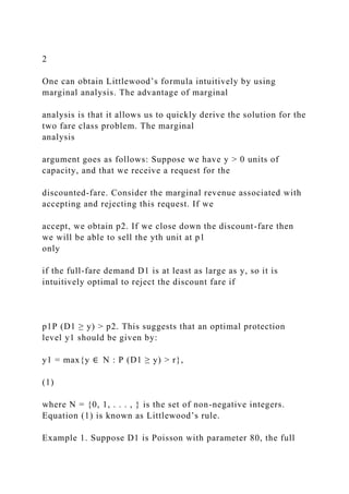
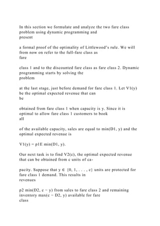
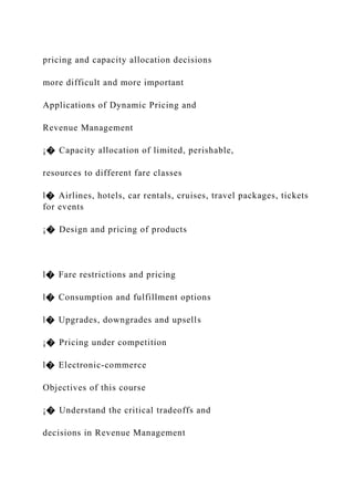
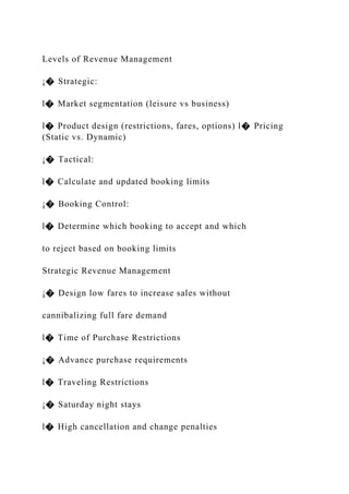
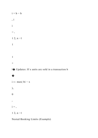
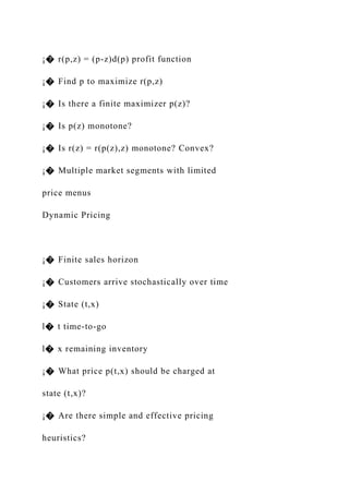
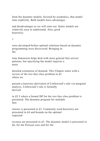
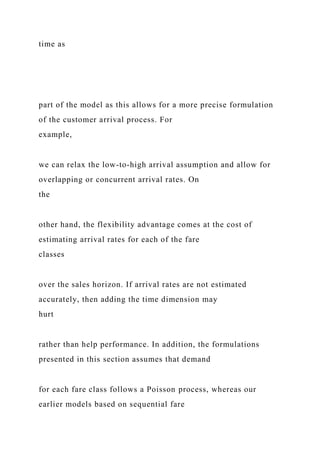
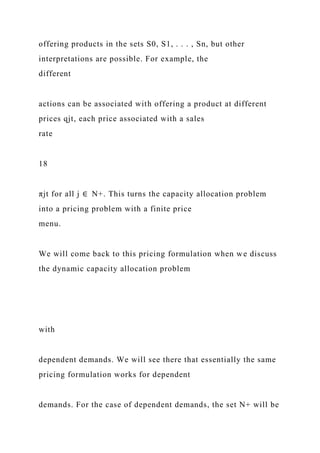
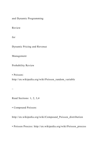
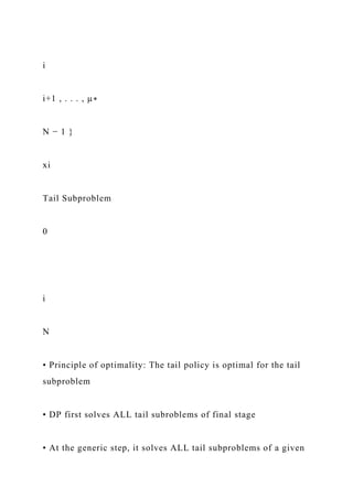
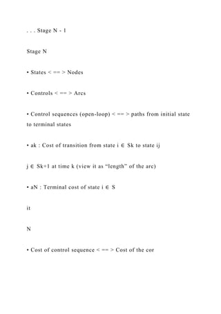
V2(c), at stage 2, to the expected revenue function V1 at stage
1. To solve for V2(c) we first need to solve
for V1(y) for y ∈ {0, 1, . . . , c}. Before moving on to the
multi-fare formulation we will provide a formal
proof of Littlewood’s rule (1), and discuss the quality of service
implications of using Littlewood’s rule
under
competition.
4
2.4
Formal Proof of Littlewood’s Rule
For any function f (y) over the integers, let ∆f (y) = f (y) − f (y
− 1). The following result will help us to
determine ∆V (y) and ∆W (y, c) = W (y, c) − W (y − 1, c).
Lemma 1 Let g(y) = EG(min(X, y)) where X is an integer
valued random variable with E[X] < ∞ and G
is an arbitrary function defined over the integers. Then
∆g(y) = ∆G(y)P (X ≥ y).
Let r(y) = ER(max(X, y)) where X is an integer valued random
variable with E[X] < ∞ and R is an
arbitrary
function defined over the integers. Then

∆r(y) = ∆R(y)P (X < y).
An application of the Lemma 1 yields the following proposition
that provides the desired formulas for
∆V1(y) and ∆W (y, c).
Proposition 1
∆V1(y) = p1P (D1 ≥ y)
y ∈ {1, . . . , }
∆W (y, c) = [∆V1(y) − p2]P (D2 > c − y)
y ∈ {1, . . . , c}.
The proof of the Lemma 1 and Proposition 1 are relegated to the
Appendix. With the help of Proposition 1
we can now formally establish the main result for the Two-Fare
Problem.
Theorem 1 The function W (y, c) is unimodal in y and is
maximized at y(c) = min(y1, c) where
y1 = max{y ∈ N : ∆V1(y) > p2}.
Moreover, V2(c) = W (y(c), c).
Proof: Consider the expression in brackets for ∆W (y, c) and
notice that the sign of ∆W (y, c) is
determined

by ∆V1(y) − p2 as P (D2 > c − y) ≥ 0.Thus W (y, c) ≥ W (y − 1,
c) as long as ∆V1(y) − p2 > 0 and W (y,
c) ≤
W (y − 1, c) as long as ∆V1(y) − p2 ≤ 0. Since ∆V1(y) = p1P
(D1 ≥ y) is decreasing1 in y, ∆V1(y) − p2
changes
signs from + to − since ∆V1(0) − p2 = p1P (D1 ≥ 0) − p2 = p1 −
p2 > 0 and limy→∞[∆V1(y) − p2] =
−p2.
This means that W (y, c) is unimodal in y. Then
y1 = max{y ∈ N : ∆V1(y) > p2}.
coincides with Littlewood’s rule (1).
When restricted to {0, 1, . . . , c}, W (y, c) is maximized at y(c)
=
min(c, y1). Consequently, V2(c) = maxy∈ {0,1,...,c} W (y, c) =
W (y(c), c), completing the proof.
2.5
Quality of Service, Spill Penalties, Callable Products and
Salvage Values
Since max(y1, c − D2) units of capacity are available for fare
class 1, at least one fare class 1 customer
will be
denied capacity when D1 > max(y1, c − D2). The probability of
this happening is a measure of the quality
of

service to fare class 1, known as the full-fare spill rate.
Brumelle et al. [4] have observed that
P (D1 > max(y1, c − D2)) ≤ P (D1 > y1) ≤ r < P (D1 ≥ y1).
(4)
They call P (D1 > y1) the maximal spill rate. Notice that if the
inequality y1 ≥ c − D2 holds with high
probability, as it typically does in practice when D2 is large
relative to c, then the spill rate approaches
the
1We use the term increasing and decreasing in the weak sense.
5
maximal flight spill rate which is, by design, close to the ratio
r. High spill rates may lead to the loss of
full-fare customers to competition. To see this, imagine two
airlines each offering a discount fare and a
full-
fare in the same market where the fare ratio r is high and
demand from fare class 2 is high. Suppose
Airline
A practices tactically optimal Revenue Management by applying
Littlewood’s rule with spill rates close
to

r. Airline B can protect more seats than recommended by
Littlewood’s rule. By doing this Airline B will
sacrifice revenues in the short run but will attract some of the
full-fare customers spilled by Airline A.
Over
time, Airline A may see a decrease in full-fare demand as a
secular change and protect even fewer seats
for
full-fare passengers. In the meantime, Airline B will see an
increase in full-fare demand at which time it
can
set tactically optimal protection levels and derive higher
revenues in the long-run. In essence, Airline B
has
(correctly) traded discount-fare customers for full-fare
customers with Airline A.
One way to cope with high spill rates and its adverse strategic
consequences is to impose a penalty cost
ρ for each unit of full-fare demand in excess of the protection
level. This penalty is suppose to measure
the
ill-will incurred when capacity is denied to a full-fare customer.
This results in a modified value function
V1(y) = p1E min(D1, y) − ρE[(D1 − y)+] = (p1 + ρ)E min(D1,
y) − ρED1. From this it is easy to see that

∆V1(y) = (p + ρ)P (D1 ≥ y), resulting in
∆W (y, c) = [(p1 + ρ)P (D1 ≥ y) − p2]P (D2 > c − y)
and
p2
y1 = max y ∈ N : P (D1 ≥ y) >
.
(5)
p1 + ρ
Notice that this is just Littlewood’s rule applied to fares p1 + ρ
and p2, resulting in fare ratio p2/(p1 + ρ)
and,
consequently, lower maximal spill rates. Obviously this
adjustment comes at the expense of having higher
protection levels and therefore lower sales at the discount-fare
and lower overall revenues.
Consequently, an
airline that wants to protect its full-fare market by imposing a
penalty on rejected full-fare demand does it
at
the expense of making less available capacity for the discount-
fare and less expected revenue. One way to
avoid

sacrificing sales at the discount-fare and improve the spill rate
at the same time is to modify the discount-
fare
by adding a restriction that allows the provider to recall or buy
back capacity when needed. This leads to
revenue management with callable products; see Gallego, Kou
and Phillips [12]. Callable products can
be
sold either by giving customers an upfront discount or by giving
them a compensation if and when
capacity
is recalled. If managed correctly, callable products can lead to
better capacity utilization, better service
to
full-fare customers and to demand induction from customers
who are attracted to either the upfront
discount
or to the compensation if their capacity is recalled.
The value function V1(y) may also be modified to account for
salvage values (also known as the
‘distressed
inventory problem’). Suppose there is a salvage value s < p2 on
excess capacity after the arrival of the
full-fare
demand (think of standby tickets or last-minute travel deals).

We can handle this case by modifying V1(y)
to
account for the salvaged units. Then V1(y) = p1E min(D1, y) +
sE(y − D1)+ = (p1 − s)E min(D1, y) + sy,
so
∆V1(y) = (p1 − s)P (D1 ≥ y) + s, resulting in
∆W (y, c) = [(p1 − s)P (D1 ≥ y) − (p2 − s)]P (D2 > c − y)
and
p2 − s
y1 = max y ∈ N : P (D1 ≥ y) >
.
(6)
p1 − s
Notice that this is just Littlewood’s rule applied to net fares p1
− s and p2 − s. This suggests that a
problem
with salvage values can be converted into a problem without
salvage values by using net fares pi ← pi −
s,
i = 1, 2 and then adding cs to the resulting optimal expected
revenue V2(c) in excess of salvage values.
3

Multiple Fare Classes: Exact
Solution
In this section we present an exact solution to the muli-fare
class problem using dynamic programming.
We
assume that the capacity provider has c units of perishable
capacity to be allocated among n fares indexed
6
so pn < . . . < p1. Lower fares typically have severe time of
purchase and traveling restrictions and may
have
restricted advanced selection that denies access to the more
desirable capacity. Given the time-of-

purchase
restriction, it is natural to assume that demands for fare classes
arrive in n stages, with fare class n
arriving
first, followed by n − 1, with fare class 1 arriving last. Let Dj
denote the random demand for fare class
j ∈ N = {1, . . . , n}. We assume that, conditional on the given
fares, the demands D1, . . . , Dn are
independent
random variables with finite means µj = E[Dj] j ∈ N . The
independent assumption is approximately
valid
in situations where fares are well spread and there are
alternative sources of capacity. Indeed, a customer
who finds his preferred fare closed is more likely to buy the
same fare for an alternative flight (perhaps
with
a competing carrier) rather than buying up to the next fare class

if the difference in fare is high. The case
of
dependent demands, where fare closures may result in demand
recapture, will be treated in a different
chapter.
The use of Dynamic Programming for the multi-fare problem
with discrete demands is due to Wollmer
[22].
Curry [6] derives optimality conditions when demands are
assumed to follow a continuos distribution.
Brumelle
and McGill [5] allow for either discrete or continuous demand
distributions and makes a connection with
the
theory of optimal stopping.
Let Vj(x) denote the maximum expected revenue that can be
obtained from x ∈ {0, 1, . . . , c} units of
capacity from fare classes {j, . . . , 1}. The sequence of events

for stage j are as follows:
1. Decide the protection level, say y ≤ x, for fares j − 1, j − 2, .
. . , 1 thus allowing at most x − y units of
fare j demand.
2. The realization of the demand Dj occurs, and we observe
min(Dj, x − y) sales at fare j.
3. The revenue pj min(Dj, x−y) is collected, and we proceed to
the beginning of stage j −1 with a
remaining
capacity of max(x − Dj, y).
The revenue from this process is
Wj(y, x) = pjE min(Dj, x − y) + EVj−1 (max(x − Dj, y)) .
(7)

We can think of Wj(y, x) as the expected revenue from x units
of capacity prior to seeing the demand for
fare
class j when up to x − y units are allowed to book at fare j and
an optimal policy is followed thereafter.
This
leads to the dynamic programming recursion
Vj(x)
=
max
Wj(y, x)
y∈ {0,1,...,x}
=
max
{pjE min(Dj, x − y) + EVj−1(max(x − Dj, y))} .

(8)
y∈ {0,1,...,x}
The dynamic program simply states that the optimal value
function is the sum of the expected revenues
from fare class j plus the expected revenues from fare classes j
− 1, . . . , 1 evaluated at the protection
level that
maximizes this sum. Notice that once we are at the beginning of
stage j − 1 we face a similar problem
over the
remaining j − 1 fare classes. Vj(x) is then the maximum
expected revenue that can be obtained from x units
of
capacity for the j-fare problem. Consequently Vn(c) is the
maximum expected revenue for the n-fare

problem
with capacity c. The recursion can be started with V0(x) = 0 if
there are no salvage values or penalties
for
spill. Alternatively, the recursion can start with V1(x) = p1E
min(D1, x) + sE[(x − D1)+] − ρE[(D1 −
x)+] for
x ≥ 0 if there is a salvage value s per unit of excess capacity
and a penalty ρ per unit of fare class 1
demand
that is denied.
3.1
Structure of the Optimal Policy
In order to analyze the structure of the optimal policy, we begin
by describing a few properties of the
value
function.

As a convention we set V0 ≡ 0. A function V (y) defined on y ∈
N is concave if ∆V (y) =
V (y) − V (y − 1) is decreasing in y ∈ N+.
7
Lemma 2 For any j ≥ 1,
a) ∆Vj(y) = Vj(y) − Vj(y − 1) is decreasing in y ∈ N+, so the
marginal value of capacity is diminishing.
b) ∆Vj(y) is increasing in j ∈ {1, . . . , n} so the marginal value
of capacity increases when we have more
stages to go.
The proof of Lemma 2 is in the Appendix. Using the Lemma we
can characterize an optimal policy as
stated in the following theorem. For the purpose of simplifying
notation we will extend the definition of
∆Vj(y)

to y = 0 by setting ∆Vj(0) = ∆V1(0) = p1 just as we did for j =
1.
Theorem 2 The function Wj(y, x) is unimodal in y and it is
maximized at min(yj−1, c), where the nested
protection levels 0 = y0 ≤ y1 ≤ y2 ≤ · · · ≤ yn−1 are given by
yj = max{y ∈ N : ∆Vj(y) > pj+1} j = 1, . . . , n − 1.
(9)
The optimal value functions are given by
Vj(x) = Wj(min(x, yj−1), x) j = 1, . . . , n, x ∈ N .
(10)
Moreover, Vj(x) is concave in x ∈ N for each j = 1, . . . , n.
Proof: An algebraic argument similar to that used to justify
Littlewood’s rule for n = 2, reveals that for

y ∈ {1, . . . , x}
∆Wj(y, x) = Wj(y, x) − Wj(y − 1, x) = [∆Vj−1(y) − pj] P (Dj > x
− y).
Let yj−1 = max{y ∈ N : ∆Vj−1(y) > pj}. By part a) of Lemma 2,
∆Vj−1(y) is decreasing in y so ∆Vj−1(y)
−
pj > 0 for all y ≤ yj−1 and ∆Vj−1(y) − pj ≤ 0 for all y > yj−1.
Consequently, if x ≤ yj−1 then ∆Wj(y, x) ≥
0
for all y ∈ {1, . . . , x} implying that Vj(x) = Wj(x, x).
Alternatively, if x > yj−1 then ∆Wj(y, x) ≥ 0
for y ∈ {1, . . . , yj} and ∆Wj(y, x) ≤ 0 for y ∈ {yj−1 + 1, . . . ,
x} implying Vj(x) = Wj(yj−1, x). Since
∆Vj(x) = ∆Vj−1(x) on x ≤ yj−1, it follows that ∆Vj(yj−1) =
∆Vj−1(yj−1) > pj > pj+1, so yj ≥ yj−1. The
concavity of Vj(x) is is equivalent to ∆Vj(x) decreasing in x,
and this follows directly from part a) of
Lemma 2.

Remarks:
1. Notice that the unconstrained protection level yj−1 is
independent of the demands Dk, k ≥ j as observed
before in the two fare setting (Littlewood’s Rule).
2. We can think of yj, j = 1, . . . , n − 1 as the unconstrained
protection levels. If we start stage j with xj
units of capacity, the constrained protection level for fares {j −
1, . . . , 1} is min(xj, yj−1). Thus capacity
is made available to fare j only if xj > yj−1.
3. The policy is implemented as follows. At stage n we start
with xn = c units of inventory, and we protect
yn−1(xn) = min(xn, yn−1) units of capacity for fares {n − 1, . . .
, 1} by allowing up to (xn − yn−1)+ units
to be sold at fare pn. Since min(Dn, (xn −yn−1)+) units are sold
during stage n, we start stage n−1 with

xn−1 = xn − min(Dn, (xn − yn−1)+). We protect yn−2(xn−1) =
min(xn−1, yn−2) units of capacity for
fares {n − 2, . . . , 1} and thus allow up to (xn−1 −yn−2)+ units
of capacity to be sold at pn−1. The
process
continues until we reach stage one with x1 units of capacity and
allow (x1 − y0)+ = (x1 − 0)+ = x1
to be sold at p1. Assuming discrete distributions, the
computational requirement to solve the dynamic
program for the n stages has been estimated by Talluri and van
Ryzin [20] to be of order O(nc2).
4. The concavity of Vn(c) is helpful if capacity can be procured
at a linear or convex cost because in this
case the problem of finding an optimal capacity level is a
concave problem in c.

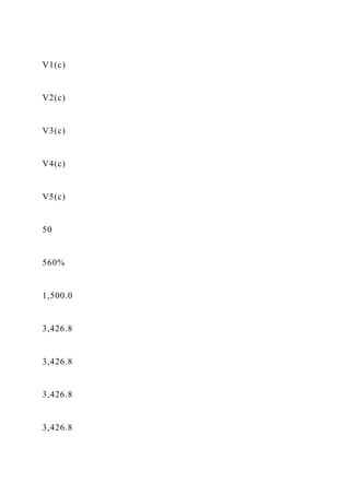
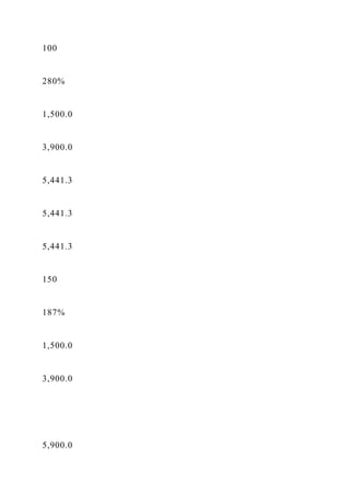
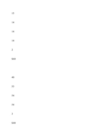
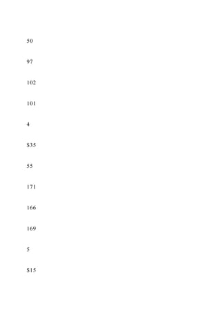
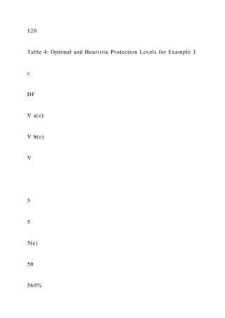
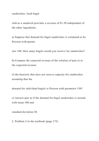
Example 3. Suppose there are five different fare classes. We
assume the demand for each of the fares is
Poisson. The fares and the expected demands are given in the
first two columns of Table 2. The third
column
includes the optimal protection levels for fares 1, 2, 3 and 4.
j
pj
E[Dj]
yj
1
$100
15

14
2
$60
40
54
3
$40
50
101
4
$35
55

169
5
$15
120
Table 2: Five Fare Example with Poisson Demands: Data and
Optimal Protection Levels
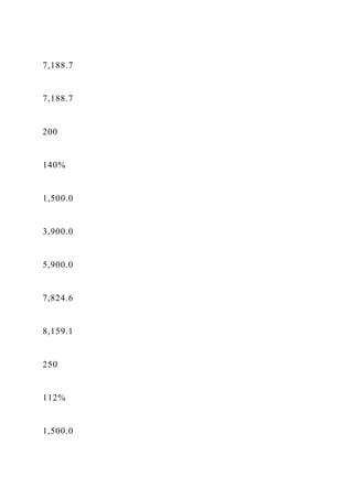
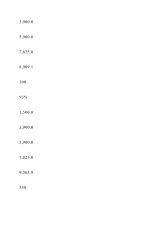
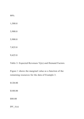
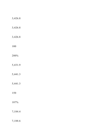
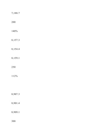
Table 3 provides the expected revenues for different capacity
levels as well as the corresponding demand
factors (
5
E[D
j=1
j ])/c = 280/c.

These results should be intuitive. Greater revenue potential is
seen as
capacity increases (since potentially more demand can be
accepted). Further, the effect of restrictions on
discounted fares is apparent in the pattern of revenue across
classes; e.g. revenue V2(50) through V5(50)
is
$3,426.8 because fare classes 3,4, and 5 are rationed since y2 =
54 > c = 50 units are protected for fare 1
and
2. However, V1(350) through V5(350) vary from $1,500 to
$9,625 because there is sufficient capacity to
accept
sales in all fare classes.
c
DF

V1(c)
V2(c)
V3(c)
V4(c)
V5(c)
50
560%
1,500.0
3,426.8
3,426.8
3,426.8
3,426.8

100
280%
1,500.0
3,900.0
5,441.3
5,441.3
5,441.3
150
187%
1,500.0
3,900.0
5,900.0

7,188.7
7,188.7
200
140%
1,500.0
3,900.0
5,900.0
7,824.6
8,159.1
250
112%
1,500.0

3,900.0
5,900.0
7,825.0
8,909.1
300
93%
1,500.0
3,900.0
5,900.0
7,825.0
9,563.9
350

80%
1,500.0
3,900.0
5,900.0
7,825.0
9,625.0
Table 3: Expected Revenues Vj(c) and Demand Factors
Figure 1 shows the marginal value as a function of the
remaining resources for the data of Example 3.
$120.00
$100.00
$80.00
DV_1(x)

DV_2(x)
$60.00
DV_3(x)
DV_4(x)
DV_5(x)
$40.00
$20.00
$-‐
0
20
40
60

80
100
120
140
160
Figure 1: ∆Vj(x), x = 1, . . . , 350, j = 1, 2, 3, 4, 5 for Example
3
9
3.2
Speeding up the Computation of the Value Function
While the value functions Vj(x), j ∈ {1, . . . , n}, x ∈ {1, . . .
c}, can be computed recursively there are
some

tricks to speed up the computations. Here we focus on how to
efficiently update ∆Vj+1(x) from ∆Vj(x).
The
key idea is to express ∆Vj+1(x) for x > yj in terms of previously
computed values of ∆Vj(x). The proof of
Proposition 2 is in the Appendix.
Proposition 2
∆V
∆V
j (x)
if x = 1, . . . , yj
j+1(x) =
E min(∆Vj(x − Dj+1), pj+1)
if x = yj + 1, . . ..

Since ∆Vj+1(x) = ∆Vj(x) for x ≤ yj, we only need to worry
about ∆Vj+1(x) for x > yj. The following
corollary to Proposition 2 makes the formula for ∆Vj+1(x), x >
yj more explicit.
Corollary 1
k−1
∆Vj+1(yj + k) = pj+1P (Dj+1 ≥ k) +
∆Vj(yj + k − i)P (Dj+1 = i)
k ∈ {1, . . . , c − yj}.
i=0
3.3
Linear and Convex Procurement Costs
Suppose that capacity c can be procured at a linear cost kc

before observing demands for the n fares: pn <
pn−1 < . . . < p1. How much capacity should be procured? The
objective is to find c to maximize Πn(c, k)
=
Vn(c) − kc. Let c(k) be the smallest optimizer of Πn(c, k) as a
function of the marginal cost k. The
following
Proposition characterizes c(k), shows that c(k) is decreasing in
k and relates c(pj+1) to protection level
yj for
j < n.
Proposition 3 The optimal procurement quantity at linear cost
kc is given by
c(k) = max{c ∈ N : ∆Vn(c) > k}.
Moreover, c(k) is decreasing in k, and yj = c(pj+1) for all j ∈
{1, . . . , n − 1}.
Clearly c(0) = ∞ since ∆Vn(c) ≥ ∆V1(c) = p1P (D1 ≥ c) > 0 for

all c ∈ N . At the other extreme,
c(p1) = y0 = 0 since ∆Vn(1) = p1P (D1 ≥ 1) < p1 = ∆Vn(0), so
no capacity would be purchased if k ≥ p1.
If the cost of capacity k(c) is increasing convex then Π(c, k(c))
is concave in c and
c(k) = max{c ∈ N : ∆Vn(c) − ∆k(c) > 0}.
Consider the convex cost function k(c) = K if c ≤ ¯
c and k(c) = ∞ for k > ¯
c. This may reflect the situation
where there is a fixed cost to leasing a resource with capacity ¯
c. The optimal choice is then to lease the
resource if Vn(¯
c) > K and not lease it otherwise.

3.4
Relaxing the Monotonicity of Fares
We continue to assume that demands arrive in the order Dn,
Dn−1, . . . , D1 but will relax the assumption
that
the fares are monotone p1 > p2 > . . . > pn. All of the results
work as stated, except the monotonicity of the
protection levels, if we redefine ∆Vj(0) = max{p1, . . . , pj}. It
is also possible to skip some of the
optimization
10
optimal capacity
450
400
350

300
ity 250
acap 200
C 150
100
50
0
0
10
20
30
40
50

60
70
80
90
100
cost
Figure 2: Optimal Capacity as a Function of Cost for the Data
of Example 3
steps as it is clear that yj−1 = 0 whenever pj > max(p1, . . . ,
pj−1) since it is optimal to allow all
bookings at
fare pj. The reader is referred to Robinson [18] for more details.
As an example, suppose that p3 < p2 >
p1.

Then V1(x) = p1E min(D1, x) and at stage 2 the decision is y1 =
0, so
V2(x) = p2E min(D2, x) + p1E min(D1, (x − D2)+).
Notice that
∆V2(x) = p2P (D2 ≥ x) + p1P (D2 < x ≤ D[1, 2])
so
y2 = max{y ∈ N : ∆V2(y) > p3}.
Notice that the capacity protected for fare 2 is higher than it
would be if there was no demand at fare 1.
4
Multiple Fare Classes: Commonly Used Heuristics
Several heuristics, essentially extensions of Littlewood’s rule,
were developed in the 1980’s. The most
important

heuristics are known as EMSR-a and EMSR-b, where EMSR
stands for expected marginal seat revenue.
Credit
for these heuristics is sometimes given to the American Airlines
team working on revenue management
problems
shortly after deregulation. The first published account of these
heuristics appear in Simpson [19] and
Belobaba
[2], [3]. For a while, some of these heuristics were even thought
to be optimal by their proponents until
optimal
policies based on dynamic programming were discovered in the
1990’s. By then heuristics were already
part of
implemented systems, and industry practitioners were reluctant
to replace them with the solutions
provided

by dynamic programming algorithms. There are several reasons
for this. First, people feel more
comfortable
with something they understand. Also, the performance gap
between the heuristics and the optimal
dynamic
program tends to be small. Finally, there is a feeling among
some users that the heuristics may be more
robust
to estimates of the mean and variance of demand.
Version a of the heuristic, EMSR-a, is based on the idea of
adding protection levels produced by applying
Littlewood’s rule to successive pairs of classes. At state j, we
need to decide how much capacity to
protect
for fares j − 1, . . . , 1. We can use Littlewood’s rule to decide
how much capacity to protect for fare k
demand

against fare j for k = j − 1, . . . , 1 and then add the protection
levels. More precisely, let rk,j = pj/pk and
set
yk,j = max{y ∈ N : P (Dk ≥ y) > rk,j}.
11
Then the EMSR-a heuristic will protect
j−1
ya
=
y
j−1
k,j
k=1

units of capacity for fares j − 1, . . . , 1 against fare j.
In particular, if Dk is Normal with mean µk and standard
deviation σk, then
j−1
ya
= µ[1, j − 1] +
σ
j−1
k Φ−1(1 − rk,j ),
k=1
where for any j, µ[1, j − 1] =
j−1 µ

k=1
k and sums over empty sets are zero.
Notice that the EMSR-a heuristic involves j − 1 calls to
Littlewood’s rule to find the protection level for
fares j − 1, . . . , 1. In contrast, the EMSR-b heuristic is based
on a single call to Littlewood’s rule for
each
protection level. However, using the EMSR-b heuristic requires
the distribution of D[1, j − 1] =
j−1 D
k=1
k .
This typically requires computing a convolution but in some
cases, such as the Normal or the Poisson, the
distribution of D[1, j − 1] can be easily obtained (because sums
of independent Normal or Poisson

random
variables are, respectively, Normal or Poisson). The distribution
of D[1, j − 1] is used together with the
weighted average fare
j−1
µk
¯
pj−1 =
pk µ[1, j − 1]
k=1
and calls on Littlewood’s rule to obtain protection level
yb

= max{y ∈ N : P (D[1, j − 1] ≥ y) > rb
}
j−1
j−1,j
where rb
= p
j−1,j
j / ¯
pj−1. Notice that the weighted average fare assumes that a
proportion µk/µ[1, j − 1] of the
protected capacity will be sold at fare pk, k = 1, . . . , j − 1. In
the special case when demands are Normal
we
obtain

yb
= µ[1, j − 1] + σ[1, j − 1]Φ−1(1 − rb
).
j−1
j−1,j
Recall that for the Normal, variances are additive, so the
standard deviation σ[1, j − 1] =
j−1 σ2.
k=1
k
4.1
Evaluating the Performance of Heuristics

While heuristic protection levels are easy to compute,
evaluating them is as hard as solving for the
optimal
policy. The expected return of a heuristic policy based on
protection levels 0 = yh ≤ yh ≤ . . . ≤ yh
can be
0
1
n−1
computed exactly or via simulation. To compute the expected
revenues exactly, let V h(x) be the expected
profit
j
from x units of capacity from fares {j, . . . , 1} under the
heuristic policy h. Then V h(x) = W h(min(x, yh
), x)

j
j
j−1
where for all y ≤ x we define W h(y, x) = p
(max(y, x − D
j
j E min(x − y, Dj ) + EV h
j−1
j )). The following result
is a direct consequence of Proposition 2 and its corollary.
Proposition 4

∆V h(x)
if x = 1, . . . , yh
j
j
∆V h (x) =
j+1
x−yh−1
= p
j
j+1P (Dj+1 ≥ x − yh) +
∆V h(x − i)P (D
j
i=0

j
j+1 = i)
if x > yh
j
Thus, if V h(x) has already been computed then V h (x) = V
h(x) for x = 1, . . . , yh. For x > yh we can
j
j+1
j
j
j
use the recursion V h (x) = V h (x − 1) + ∆V h (x) starting with
x = yh + 1 in conjunction with the second

j+1
j+1
j+1
j
part of Proposition 4.
12
To estimate the expected revenue and other measures of
performance, such as the variance, we can also
use Monte Carlo simulation. Suppose we generate many random
copies of simulated demands (D1, . . . ,
Dn).
For each copy we compute sales (sh, . . . , sh) and revenues Rh
=
n

p
under heuristic h. Averaging
1
n
i=1
ish
i
over all the values of Rh gives an estimate of V h(c). Simulated
sales can be generated sequentially via sh
=
n
j
min(Dj, (xj −yh

)+) starting with j = n and x
.
n−1
n = c and using the capacity update formula xj = xj+1 − sh
j+1
Example 3 (continued) We have applied the EMSR-a and
EMSR-b heuristics to the data of Example 3.
Table
4 repeats the data and reports the heuristic protection levels ya,
yb as well as the optimal protection
levels.
Table 5 reports V a(c) and V b(c) as well as V
5
5

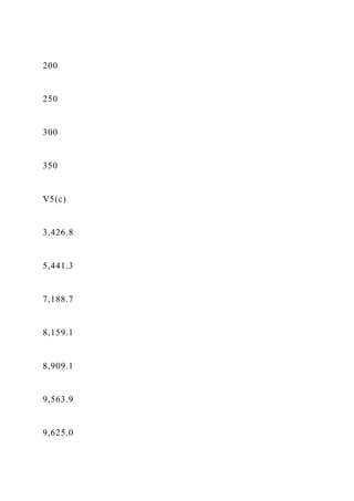
5(c) for values of c ∈ {50, 100, 150, 200, 250, 300, 350}.
j
pj
E[Dj]
ya
yb
y
j
j
j
1
$100

15
14
14
14
2
$60
40
53
54
54
3
$40

50
97
102
101
4
$35
55
171
166
169
5
$15

120
Table 4: Optimal and Heuristic Protection Levels for Example 3
c
DF
V a(c)
V b(c)
V
5
5
5(c)
50
560%

3,426.8
3,426.8
3,426.8
100
280%
5,431.9
5,441.3
5,441.3
150
187%
7,184.4
7,188.6

7,188.7
200
140%
8,157.3
8,154.4
8,159.1
250
112%
8,907.3
8,901.4
8,909.1
300

93%
9,536.5
9,536.0
9,563.9
350
80%
9,625.0
9,625.0
9,625.0
Table 5: Performance of Heuristics for Example 3
As seen in Table 5, both the EMSR-a and the EMSR-b heuristic
perform very well against Poisson
demands

under a low-to-high arrival pattern. The heuristics continue to
perform well if demands are compound
Poisson
and aggregate demands are approximated by the use of a
Gamma distribution.
However, EMSR based
heuristics can significantly underperform relative to models that
allow more general fare arrival rates.
We will
have an opportunity to revisit this issue in Section 7.
5
Bounds, Revenue Opportunity Model, and New Heuristics
In this section we develop bounds on Vn(c) which may be
useful in evaluating the potential of applying
revenue

management solutions. To obtain an upper bound, consider the
perfect foresight problem where the
demand
vector D = (D1, . . . , Dn) is known in advance. This demand
knowledge allows us to optimally allocate
capacity
by solving the following knapsack type problem
n
V U (c, D)
=
max
p
n
k xk
(11)

k=1
s.t.
xk
≤
Dk
∀
k = 1, . . . , n
n
xk
≤
c
k=1

xk
≥
0
∀
k = 1, . . . , n.
13
Clearly, for each realization of D, advance knowledge results in
revenues that are at least as high as the
optimal
dynamic policy that does not have perfect foresight. As a result,
Vn(c) ≤ EV U (c, D). For convenience,
we
n
will denote this upper bound as V U (c) = EV U (c, D).

n
n
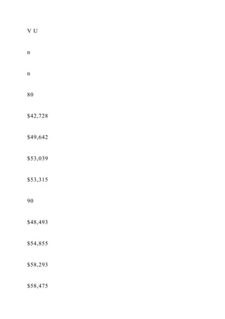
The solution to (11) can be written explicitly as xk = min(Dk, (c
− D[1, k − 1])+), k = 1, . . . , n where
for convenience we define D[1, 0] = 0. The intuition here is that
we give priority to higher fares so fare
k ∈ {1, . . . , n} gets the residual capacity (c − D[1, k − 1])+.
The expected revenue can be written more
succinctly after a few algebraic calculations:
n
V U (c)
=
p
n

k E min(Dk , (c − D[1, k − 1])+)
(12)
k=1
n
=
pk (E min(D[1, k], c) − E min(D[1, k − 1], c))
k=1
n
=
(pk − pk+1)E min(D[1, k], c)
(13)

k=1
where for convenience we define pn+1 = 0. Moreover, since V
U (c, D) is concave in D, it follows from
Jensen’s
n
inequality that V U (c) = EV U (c, D) ≤ V U (c, µ) where V U
(c, µ) is the solution to formulation (11)
with
n
n
n
n
µ = E[D] instead of D. More precisely,
n
V U (c, µ)

=
max
p
n
k xk
(14)
k=1
s.t.
xk
≤
µk

∀
k = 1, . . . , n
n
xk
≤
c
k=1
xk
≥
0
∀
k = 1, . . . , n.
The linear program (14) is known as the fluid model or the

deterministic capacity allocation problem. It
is
essentially a knapsack problem whose solution can be given in
closed form xk = min(µk, (c − µ[1, k −
1])+) for
all k = 1, . . . , n. Consequently, V U (c) ≤ V U (c, µ) =
n
(p
n
n
k=1
k − pk+1) min(µ[1, k], c).
A lower bound can be obtained by assuming a low to high
arrival pattern with zero protection levels.

This gives rise to sales min(Dk, (c − D[k + 1, n])+) at fare k =
1, . . . , n and revenue lower bound V L(c,
D) =
n
p
k=1
k E min(Dk , (c − D[k + 1, n])+).
Taking expectations we obtain
n
V L(c)
=
p
n

k E min(Dk , (c − D[k + 1, n])+)
(15)
k=1
n
=
pk (E min(D[k, n], c) − E min(D[k + 1, n], c))
k=1
n
=
(pk − pk−1)E min(D[k, n], c)
(16)
k=1

where p0 = 0. Notice that all of the terms in the sum are
negative except for k = 1. Clearly V L(c) ≤ V
n
n(c)
since the expected revenue is computed under sub-optimal
protection levels. The above arguments justify
the
main result of this section.
14
Proposition 5
V L(c) ≤ V
(c) ≤ V U (c, µ)
(17)
n

n(c) ≤ V U
n
n
Of course, the bounds require the computation of E min(D[1, k],
c), k = 1, . . . , n. However, this is often
an easy computation. Indeed, if D[1, k] is any non-negative
integer random variable then E min(D[1, k], c)
=
c
P (D[1, k] ≥ j). If D[1, k] is Normal we can take advantage of
the fact that E min(Z, z) = z(1 − Φ(z)) −
j=1
φ(z) when Z is a standard Normal random variable and φ is the
standard Normal density function. If
follows

that if D[1, k] is Normal with mean µ and variance σ2, then
E min(D[1, k], c) = µ + σE min(Z, z) = µ + σ [z(1 − Φ(z)) −
φ(z)]
where z = (c − µ)/σ.
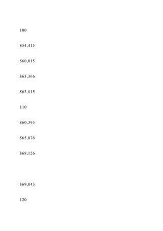
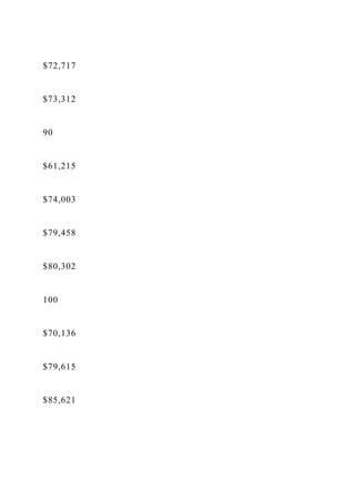
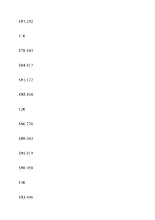
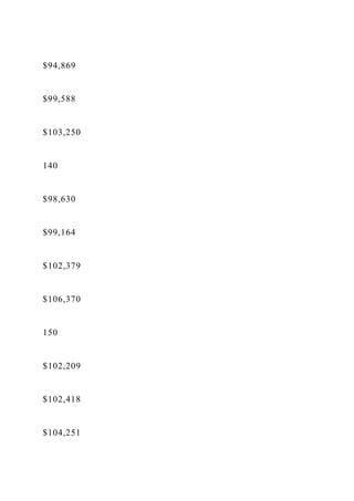
Tables 6 and 7 report V L(c), V
(c) and V
n
n(c), V U
n
n(c, µ) for the data of Examples 4 and 5, respectively.
Notice that V U (c) represents a significant improvement over
the better known bound V
n

n(c, µ), particularly
for intermediate values of capacity. The spread V U (c) − V
L(c) between the lower and upper bound is a
n
n
gauge of the potential improvements in revenues from using an
optimal or heuristic admission control
policy.
When capacity is scarce relative to the potential demand, then
the relative gap is large, and the potential
for applying revenue management solutions is also relatively
large. This is because significant
improvements
in revenues can be obtained from rationing capacity to lower
fares. As capacity increases, the relative
gap

decreases indicating that less can be gained by rationing
capacity. At very high levels of capacity it is
optimal
to accept all requests, and at this point there is nothing to be
gained from the use of an optimal admission
control policy.
c
V L(c)
V
(c)
V U (c, µ)
n
n(c)

V U
n
n
80
$42,728
$49,642
$53,039
$53,315
90
$48,493
$54,855
$58,293
$58,475

100
$54,415
$60,015
$63,366
$63,815
110
$60,393
$65,076
$68,126
$69,043
120

$66,180
$69,801
$72,380
$74,243
130
$71,398
$73,926
$75,923
$79,443
140
$75,662
$77,252
$78,618

$82,563
150
$78,751
$79,617
$80,456
$82,563
160
$80,704
$81,100
$81,564
$82,563

Table 6: Optimal Revenue and Bounds for Example 4.
c
V L(c)
V
(c)
V U n(c, µ)
n
n(c)
V U
n
80
$52,462
$67,505

$72,717
$73,312
90
$61,215
$74,003
$79,458
$80,302
100
$70,136
$79,615
$85,621

$87,292
110
$78,803
$84,817
$91,122
$92,850
120
$86,728
$89,963
$95,819
$98,050
130
$93,446

$94,869
$99,588
$103,250
140
$98,630
$99,164
$102,379
$106,370
150
$102,209
$102,418
$104,251

$106,370
160
$104,385
$104,390
$105,368
$106,370
Table 7: Optimal Revenue and Bounds for Example 5.
5.1
Revenue Opportunity Model
The bounds presented here can help with the so called Revenue
Opportunity Model (ROM). The revenue
opportunity is the spread between the optimal revenue, obtained
by hindsight using the estimated

uncensored
15
demand, and the revenue that results from not applying booking
controls. Demand uncensoring refers to a
sta-
tistical technique that attempts to estimate actual demand from
the observed sales which may be
constrained
by booking limits. The ex-post optimal revenue is a hindsight
optimization and is equivalent to our perfect
foresight model, resulting in revenue V U (c, D), where D is the
uncensored demand. On the other hand,
the
n
revenue based on not applying booking controls is just V L(c,
D), so a measure of the revenue opportunity
is

n
V U (c, D) − V L(c, D). The achieved revenue opportunity is the
difference between the actual revenue
from
n
n
applying optimal or heuristic controls and the lower bound. The
ratio of the achieved revenue opportunity
to
the revenue opportunity is often called the percentage achieved
revenue opportunity. The revenue
opportunity
V U (c, D) − V L(c, D) is sometimes approximated by V U (c) −
V L(c) to get an idea of the revenue
opportunity.
n

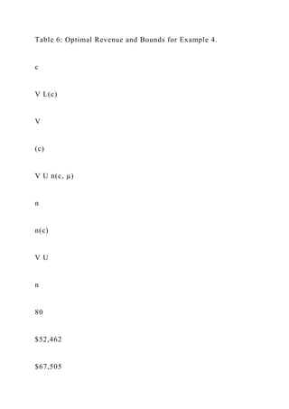
n
n
n
Table 6 and 7 shows there is significant revenue opportunity,
particularly for c ≤ 140. Thus, one use for
the
ROM is to identify situations where RM has the most potential
so that more effort can be put where is
most
needed. The ROM has also been used to show the benefits of
using leg-based control versus network-
based
controls. The reader is refer to Chandler and Ja ([8]) and to
Temath et al. ([21]) for further information on
the uses of the ROM.
5.2

Bounds Based Heuristic
It is common to use an approximation to the value function as a
heuristic. To do this, suppose that ˜
Vj(x) is
an approximation to Vj(x). Then a heuristic admission control
rule can be obtained as follows:
˜
yj = max{y ∈ N : ∆ ˜
Vj(y) > pj+1} j = 1, . . . , n − 1.
(18)
Suppose we approximate the value function Vj(x) by ˜
Vj(x) = θV L(x) + (1 − θ)V U (x) for some θ ∈ [0, 1]

j
j
and V L(x) and V U (x) are the bounds obtained in this section
applied to n = j and c = x. Notice that
j
j
∆V L(x) = p
(p
(x) =
j−1 (p
j
1P (D[1, j] ≥ x) +
j

k=2
k − pk−1)P (D[k, j] ≥ x), while ∆V U
j
k=1
k − pk+1)P (D[1, k] ≥
x) + pjP (D[1, j] ≥ x).
6
Multiple Fare Classes with Arbitrary Fare Arrival Patterns
So far we have suppressed the time dimension; the order of the
arrivals has provided us with stages that
are
a proxy for time, with the advance purchase restriction for fare j
serving as a mechanism to end stage j. In
this section we consider models where time is considered
explicitly. There are advantages of including

time as
part of the model as this allows for a more precise formulation
of the customer arrival process. For
example,
we can relax the low-to-high arrival assumption and allow for
overlapping or concurrent arrival rates. On
the
other hand, the flexibility advantage comes at the cost of
estimating arrival rates for each of the fare
classes
over the sales horizon. If arrival rates are not estimated
accurately, then adding the time dimension may
hurt
rather than help performance. In addition, the formulations
presented in this section assumes that demand
for each fare class follows a Poisson process, whereas our
earlier models based on sequential fare

arrivals do
not have this restriction. We will extend the formulation in this
section to the case of compound Poisson in
§7.
We assume that customers arrive to the system according to a
time heterogeneous Poisson process with
intensity λjt, 0 ≤ t ≤ T where T is the length of the horizon, t
represents the time-to-go and j ∈ {1, . . . , n}.
Then the number of customers that arrive during the last t units
of time and request product j, say Njt, is
t
Poisson with mean Λjt =
λ
0
jsds. For simplicity we will write Λj , instead of ΛjT , to denote

the expected
number of requests for fare j over the entire horizon [0, T ]. The
low-to-high arrival pattern can be
embedded
into the time varying model by dividing the selling horizon into
n sub-intervals [tj−1, tj], j = 1, . . . , n with
tj = jT /n, and setting λjt = nΛj/T over t ∈ [tj−1, tj] and λjt = 0
otherwise.
Let V (t, x) denote the maximum expected revenue that can be
attained over the last t units of the sale
horizon with x units of capacity. We will develop both discrete
and continuous time dynamic programs to
compute V (t, x). To construct a dynamic program we will need
the notion of functions that go to zero
faster
16

than their argument. More precisely, we say that a function g(x)
is o(x) if limx↓0 g(x)/x = 0. We will show
that the probability that over the interval [t − δt, t] there is
exactly one request and the request is for
product
j is of the form λjtδt + o(δt). To see this notice that the
probability that a customer arrives and requests
one
unit of product j over the interval [t − δt, t]is
λjtδ exp(−λjtδt) + o(δt) = λjtδt[1 − λjtδt] + o(δt) = λjtδt + o(δt),
while the probability that there are no requests for the other
products over the same interval is
exp(−
λktδt) + o(δt) = 1 −
λktδt + o(δt).

k=j
k=j
Multiplying the two terms and collecting terms we obtain λjtδt
+ o(δt) as claimed.
Recall that some fares have embedded time-of-purchase
restrictions. Let Nt ⊂ N = {1, . . . , n} to be the
set of allowable fares at time-to-go t. Usually Nt = N for large t,
but low fares are dropped from Nt as the
time-of-purchase restrictions become binding.
We can now write
V (t, x)
=
λjtδt max(pj + V (t − δt, x − 1), V (t − δt, x)) + (1 −
λjtδt)V (t − δt, x) + o(δt)

j∈ Nt
j∈ Nt
=
V (t − δt, x) + δt
λjt[pj − ∆V (t − δt, x)]+ + o(δt)
(19)
j∈ Nt
with boundary conditions V (t, 0) = 0 and V (0, x) = 0 for all x
≥ 0, where ∆V (t, x) = V (t, x) − V (t, x −
1) for
x ≥ 1 and t ≥ 0.
Subtracting V (t − δt, x) from both sides of equation (19),
dividing by δt and taking the limit as δt ↓ 0, we

obtain the following equation, known as the Hamilton Jacobi
Bellman (HJB) equation:
∂V (t, x) =
λjt[pj − ∆V (t, x)]+
(20)
∂t
j∈ Nt
with the same boundary conditions. The equation tells us that
the rate at which V (t, x) grows with t is the
weighted sum of the positive part of the fares net of the
marginal value of capacity ∆V (t, x) at state (t, x).
While the value function can be computed by solving and
pasting the differential equation (20), in practice
it is easier to understand and compute V (t, x) using a discrete
time dynamic programming formulation. A

discrete time dynamic programming formulation emerges from
(19) by rescaling time, setting δt = 1, and
dropping the o(δt) term. This can be done by selecting a > 1, so
that T ← aT is an integer, and setting
λjt ← 1 λ
λ
a
j,t/a, for t ∈ [0, aT ]. The scale factor a should be selected so
that, after scaling,
j∈ N
jt << 1,
t
e.g.,

λ
j∈ N
jt ≤ .01 for all t. The resulting dynamic program, after rescaling
time, is given by
t
V (t, x) = V (t − 1, x) +
λjt[pj − ∆V (t − 1, x)]+.
(21)
j∈ Nt
with the same boundary conditions. Computing V (t, x) via (21)
is quite easy and fairly accurate if time is
scaled appropriately. For each t, the complexity is order O(n)
for each x ∈ {1 . . . , c} so the complexity
per
period is O(nc), and the overall computational complexity is

O(ncT ).
A formulation equivalent to (21) was first proposed by Lee and
Hersh [13], who also show that ∆V (t, x)
is
increasing in t and decreasing in x. The intuition is that the
marginal value of capacity goes up if we have
more
time to sell and goes down when we have more units available
for sale. From the dynamic program (21),
it is
optimal to accept a request for product j when pj ≥ ∆V (t − 1, x)
or equivalently, when pj + V (t − 1, x −
1) ≥
V (t − 1, x), i.e., when the expecte revenue from accepting the
request exceeds the expected revenue of
denying
the request. Notice that if it is optimal to accept a request for
fare j, then it is also optimal to accept a
request

17
for any higher fare. Indeed, if pk ≥ pj and pj ≥ ∆V (t − 1, x),
then pk ≥ ∆V (t − 1, x). Assuming that the
fares
are ordered: p1 ≥ p2 ≥ . . . ≥ pn, then it is optimal to accept all
fares in the active set A(t, x) = {1, . . . ,
a(t, x)}, where
a(t, x) = max{j ∈ Nt : pj ≥ ∆V (t − 1, x)}
t ≥ 1, x ≥ 1},
and to reject all fares in the complement R(t, x) = {j ∈ {1, . . . ,
n} : j > a(t, x)}. For convenience we
define
a(t, 0) = a(0, x) = 0 and A(t, 0) = A(0, x) = ∅ . For each time-to-
go t let the protection level for fares in
{1, . . . , j} be

yj(t) = max{x : a(t, x) = j},
so if x ≤ yj(t) then fares j + 1 and higher should be closed.
Proposition 6 The active set A(t, x) is decreasing in t and
increasing in x. Moreover, yj(t) is increasing in
j and increasing in t.
Proof: Both results follow directly from the fact that ∆V (t, x) is
increasing in t and decreasing in x.
That intuition is that A(t, x) is decreasing in t because it is
optimal to open fewer fares when we have
more
time to sell capacity at higher fares. The intuition that A(t, x) is
increasing in x is that it we may need open
more fares when we have more inventory. The intuition for yj(t)
to be monotone in j is that we should
protect
at least as many units for sales of fares in {1, . . . , j + 1} than

for sales of fares in {1, . . . , j}, so yj+1(t) ≥
yj(t).
The intuition for yj(t) to be monotone in t is that with more time
to sell, say t > t, we have the potential to
sell more from set {1, . . . , j} so at least as many units should
be protected: yj(t ) ≥ yj(t).
6.1
A Pricing Formulation with Broader Interpretation
At any time t, let λt =
n
λ
λ
j=1

jt be the overall arrival rate at time t.
Define πjt =
j
k=1
kt/λt and
rjt =
j
p
k=1
k λkt/λt.
We can think of πjt and rjt as the probability of sale and the
average revenue rate,
per arriving customer, when we offer all the fares in the
consecutive set Sj = {1, . . . , j}. For

convenience,
let π0t = r0t = 0 denote, respectively, the sales rate and the
revenue rate associated with S0 = ∅ . Now let
qjt = rjt/πjt be the average fare per unit sold when the offer set
is Sj. If πjt = 0, we define qjt = 0. This
implies that πjt[qjt − ∆V (t − 1, x)] is zero whenever πjt = 0,
e.g., when j = 0.
Let N + = N
t
t ∪ {0}. With this notation, we can write formulation (21) as
V (t, x)
=
V (t − 1, x) + λt max [rjt − πjt∆V (t − 1, x)]
j∈ N +

t
=
V (t − 1, x) + λt max πjt[qjt − ∆V (t − 1, x)].
(22)
j∈ N +
t
The reason to include 0 as a choice is that for j = 0, the term
vanishes and this allow us to drop the
positive
part that was present in formulation (21). The equivalent
formulation for the continuous time model (20)
is
∂V (t, x) = λt max πjt[qjt − ∆V (t, x)].
(23)

∂t
j∈ N +
t
These formulation suggest that we are selecting among the
actions S0, S1, . . . , Sn to maximize the sales
rate
πjt times the average fare qjt net of the marginal value of
capacity (∆V (t − 1, x) for model (22) and ∆V (t,
x)
for model (23)). In essence, the problem has been reduced to a
pricing problem with a finite price menu.
Formulations (22) and (23) can be interpreted broadly as the
problem of optimizing the expected revenue
from state (t, x) where there are a finite number of actions.
These actions can be, as above, associated
with

offering products in the sets S0, S1, . . . , Sn, but other
interpretations are possible. For example, the
different
actions can be associated with offering a product at different
prices qjt, each price associated with a sales
rate
18
πjt for all j ∈ N+. This turns the capacity allocation problem
into a pricing problem with a finite price
menu.
We will come back to this pricing formulation when we discuss
the dynamic capacity allocation problem
with
dependent demands. We will see there that essentially the same
pricing formulation works for dependent
demands. For the case of dependent demands, the set N+ will be

the index corresponding to a collection
of
sets that is efficient in a sense that will be made precise later.
7
Compound Poisson Demands
The formulations of the dynamic programs (20) and (21),
implicitly assume that each request is for a
single
unit. Suppose instead, that each arrival is for a random number
of units. More specifically, suppose that
request for fare j are of random size Zj, and that the probability
mass function Pj(z) = P (Zj = z), z ≥ 1 is
known for each j. As before, we assume independent demands
for the different fare classes j ∈ N . We
seek
to generalize the dynamic programs (20) and (21) so that at each
state (t, x) we can decide whether or not

to
accept a fare pj request of size Zj = z. The expected revenue
from accepting the request is zpj + V (t − 1, x
− z)
and the expected revenue from rejecting the request is V (t − 1,
x). Let ∆zV (t, x) = V (t, x) − V (t, x − z)
for
all z ≤ x and ∆zV (t, x) = ∞ if z > x. We can think of ∆zV (t, x)
as a the sum of the the z marginal values
∆V (t, x) + ∆V (t, x − 1) + . . . + ∆V (t, x − z + 1).
The dynamic program (20) with compound Poisson demands is
given by
∞
∂V (t, x) =
λjt
Pj(z)[zpj − ∆zV (t, x)]+,

(24)
∂t
j∈ Nt
z=1
while the dynamic program (21) with compound Poisson
demands is given by
∞
V (t, x) = V (t − 1, x) +
λjt
Pj(z)[zpj − ∆zV (t − 1, x)]+,
(25)
j∈ Nt

z=1
with boundary conditions V (t, 0) = V (0, x) = 0. Notice that the
sums in (24) and (25) can be changed to
x
z=1
∞
instead of
as the terms z > x do not contribute to the sum given our
convention that ∆
z=1
z V (t, x) = ∞ for
x > z. The optimal policies for the two programs are,
respectively, to accept a size z request fare pj, j ∈
Nt,

if zpj ≥ ∆zV (t, x), and to accept a z request fare pj, j ∈ Nt, if
zpj ≥ ∆zV (t − 1, x). The two policies
should
largely coincide time is scaled correctly so that
λ
j∈ N
jt << 1 for all t ∈ [0, T ].
t
For compound Poisson demands, we can no longer claim that
the marginal value of capacity ∆V (t, x) is
decreasing in x, although it is still true that ∆V (t, x) is
increasing in t. To see why ∆V (t, x) is not
monotone in
x, consider a problem where the majority of the requests are for
two units and request are seldom for one

unit.
Then the marginal value of capacity for even values of x may be
larger than the marginal value of capacity
for
odd values of x. Consequently, some of the structure may be
lost. For example, it may be optimal to
accept a
request of a single unit of capacity when x is odd, but not if x is
even, violating the monotonicity of ∆V (t,
x).
However, even if some of the structure is lost, the computations
involved to solve (25) are
straightforward as
long as the distribution of Zj is known. Airlines, for example,
have a very good idea of the distribution of
Zj
for different fare classes that may depend on the market served.
Example 4. Consider again the data of Examples 3 with fares p1

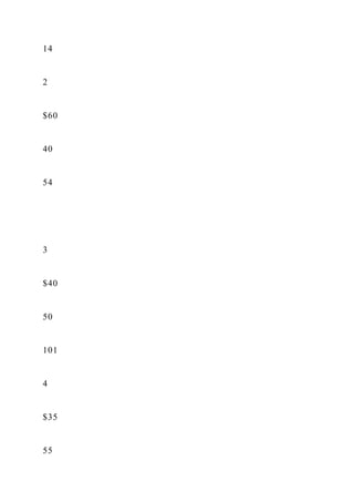
= $100, p2 = $60, p3 = $40, p4 = $35
and
p5 = $15 with independent compound Poisson demands, with
uniform arrival rates λ1 = 15, λ2 = 40, λ3 =
50, λ4 = 55, λ5 = 120 over the horizon [0, 1]. We will assume
that Nt = N for all t ∈ [0, 1]. The aggregate
arrival rates are given by Λj = λjT = λj for all j. We will assume
that the distribution of the demand sizes
is
given by P (Z = 1) = 0.65, P (Z = 2) = 0.25, P (Z = 3) = 0.05
and P (Z = 4) = .05 for all fare classes.
Notice
that E[Z] = 1.5 and E[Z2] = 2.90, so the variance to mean ratio
is 1.933. We used the dynamic program
(25) with a rescaled time horizon T ← aT = 2, 800, and rescaled
arrival rates λj ← λj/a for all j. Table 8
provides the values V (T, c) for c ∈ {50, 100, 150, 200, 250,
300, 350}. Table 8 also provides the

values ∆V (t, x)
19
for t = 207 in the rescaled horizon for x ∈ {1, . . . , 6} to
illustrate the behavior of the policy. The reader
can
verify that at state (t, x) = (208, 3) it is optimal to accept a
request for one unit at fare p2, and to reject the
request if it is for two units. Conversely, if the state is (t, x) =
(208, 4) then it is optimal to reject a request
for one unit at fare p2, and to accept the request if it is for two
units. The reason for this is that the value
of
∆V (t, x) is not monotone decreasing at x = 4.
c
50

100
150
200
250
300
V (T, c)
$3,837
$6,463
$8,451
$10,241
$11,724
$12,559

x
1
2
3
4
5
6
∆V (t, x)
70.05
66.48
59.66
60.14

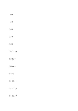
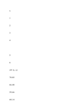
54.62
50.41
Table 8: Value function V (T, c) and marginal revenues ∆V (t,
c) for Example 4: Compound Poisson
7.1
Static vs Dynamic Policies
Let Nj be the random number of request arrivals for fare j over
the horizon [0, T ], Then Nj is Poisson
with
T
parameter Λj =
λ
0
jtdt. Suppose each arrival is of random size Zj . Then the

aggregate demand, say Dj , for
fare j is equal to
Nj
Dj =
Zjk,
(26)
k=1
where Zjk is the size of the kth request. It is well known that
E[Dj] = E[Nj]E[Zj] = ΛjE[Zj] and that
Var[Dj] = E[Nj]E[Z2] = Λ
], where E[Z2] is the second moment of Z
j

j E[Z 2
j
j
j . Notice that Jensen’s inequality
implies that the the variance to mean ratio E[Z2]/E[Z
j
j ] ≥ E[Zj ] ≥ 1.
In practice, demands D1, . . . , Dn are fed, under the low-to-
high arrival assumption, into static policies to
compute Vj(c), j = 1, . . . , n and protection levels yj, j = 1, . . .
, n − 1 using the dynamic program (8), or
to
the EMSR-b heuristic to compute protection levels yb, . . . , yb
. Since the compound Poisson demands are

1
n−1
difficult to deal with numerically, practitioners often
approximate the aggregate demands Dj by a Gamma
distribution with parameters αj and βj, such that αjβj =
E[Nj]E[Zj] and αjβ2 = E[N
], yielding
j
j ]E[Z 2
j
αj = ΛjE[Zj]2/E[Z2], and β
]/E[Z
j

j = E[Z 2
j
j ].
We are interested in comparing the expected revenues obtained
from static policies to those of dynamic
policies. More precisely, suppose that that demands are
compound poisson and Dj is given by (26) for
every
j = 1, . . . , n. Suppose that protection levels y1, y2, . . . , yn−1
are computed using the low-to-high static
dynamic program (8) and let yb, yb, . . . , yb
be the protection levels computed using the EMSR-b heuristic.
Protection
1
2

n−1
levels like these are often used in practice in situations where
the arrival rates λjt, t ∈ [0, T ], j = 1, . . . ,
n, are not necessarily low-to-high. Two possible
implementations are common. Under theft nesting a size
z request
for fare class j as state (t, x) is accepted if x − z ≥ yj−1. This
method is called theft nesting because the
remaining inventory x at time-to-go t is x = c − b[1, n] includes
all bookings up to time-to-go t, including
bookings b[1, j − 1]. Standard nesting counts only bookings for
lower fare classes and is implemented by
accepting a size z request for fare j at state (t, x) if x − z ≥
(yj−1 − b[1, j − 1])+, where b[1, j − 1] are the
observed bookings of fares [1, j − 1] up to state (t, x). When c >
yj−1 > b[1, j − 1], this is equivalent to
accepting a request for z units for fare j if c − b[j, n] − z ≥ yj−1,
or equivalently if b[j, n] + z ≤ c − yj−1,

so
only bookings of low fares count. In practice, standard nesting
works much better than theft nesting when
the arrival pattern is not low-to-high.
Notice that the expected revenue, say V s(T, c), resulting from
applying the static protection levels y1, . . .
, yn−1
with theft nesting is not, in general, equal to Vn(c), the optimal
expected revenue when the arrivals are
low-
to-high. Similarly, the expected revenue, say V b(T, c),
resulting from applying the EMSR-b protection
levels
yb, . . . , yb
with theft nesting is not, in general, equal to V b(c), the

expected revenue when the arrivals are
1
n−1
n
low-to-high.
The next proposition shows that V s(T, x) ≤ V (T, x), where V
(T, x) is the optimal expected revenue for
the
compound Poisson Dynamic Program. The same simple proof
can be used to show that V b(T, x) ≤ V (T,
x).
20
In fact, a proof is hardly needed as we are comparing heuristics
to optimal dynamic policies.
Proposition 7

V s(T, x) ≤ V (T, x) ∀ x ∈ {0, 1, . . . , c}.
Proof: Clearly for V s(0, x) = V (0, x) = 0 so the result holds for
t = 0, for all x ∈ {0, 1, . . . , c}. Suppose
the result holds for time-to-go t − 1, so V s(t − 1, x) ≤ V (t − 1,
x) for all x ∈ {0, 1, . . . , c}. We will show
that it also holds for time-to-go t. If a request of size z arrives
for fare class j, at state (t, x), the policy
based on
protection levels y1, . . . , yn−1 will accept the request if x − z
≥ (yj−1 − b[1, j − 1])+ and will rejected
otherwise.
In the following equations, we will use Qj(z) to denote P (Zj >
z). We have
x−(yj−1−b[1,j−1])+
V s(t, x)
=
λjt[

Pj(z)(zpj + V s(t − 1, x − z))
j∈ Nt
z=1
+
Qj(x − (yj−1 − b[1, j − 1])+)V s(t − 1, x)] + (1 −
λjt)V s(t − 1, x)
j∈ Nt
x−(yj−1−b[1,j−1])+
≤
λjt[
Pj(z)(zpj + V (t − 1, x − z))

j∈ Nt
z=1
+
Qj(x − (yj−1 − b[1, j − 1])+)V (t − 1, x)] + (1 −
λjt)V (t − 1, x)
j∈ Nt
x−(yj−1−b[1,j−1])+
=
V (t − 1, x) +
λjt
Pj(z)(zpj − ∆zV (t − 1, x))
j∈ Nt
z=1

∞
≤
V (t − 1, x) +
λjt
Pj(z)(zpj − ∆zV (t − 1, x))+
j∈ Nt
z=1
=
V (t, x),
where the first equation follows from the application of the
protection level policy, the first inequality
follows

from the inductive hypothesis V s(t − 1, x) ≤ V (t − 1, x). The
second equality collects terms, the second
inequality follows because we are taking positive parts, and the
last equality from the definition of V (t,
x).
While we have shown that V s(T, c) ≤ V (T, c), one may wonder
whether there are conditions where
equality
holds. The following results answers this question.
Corollary 2 If the Dj’s are independent Poisson random
variables and the arrivals are low-to-high then
Vn(c) = V s(T, c) = V (T, c).
Proof: Notice that if the Djs are Poisson and the arrivals are
low-to-high, then we can stage the arrivals
so that λjt = nE[Dj]/T over t ∈ (tj−1, tj] where tj = jT /n for j =
1, . . . , n. We will show by induction in
j that Vj(x) = V (tj, x). Clearly y0 = 0 and V1(x) = p1E min(D1,

x) = V (t1, x) assuming a sufficiently
large
rescale factor. Suppose, by induction, that Vj−1(x) = V (tj−1,
x). Consider now an arrival at state (t, x)
with
t ∈ (tj−1, tj]. This means that an arrival, if any, will be for one
unit of fare j. The static policy will accept
this
request if x − 1 ≥ yj−1, or equivalently if x > yj−1. However, if
x > yj−1, then ∆(t − 1, x) ≥ ∆V (tj−1, x) ≥
pj, because ∆V (t, x) is increasing in t and because yj−1 =
max{y : ∆Vj−1(y) > pj} = max{y : ∆V (tj−1, x)
> pj},
by the inductive hypothesis. Conversely, if the dynamic
program accepts a request, then pj ≥ ∆V (t, x) and
therefore x > yj−1 on account of ∆V (t, x) ≥ ∆V (tj−1, x).
We have come a long way in this chapter and have surveyed

most of the models for the independent
demand case. Practitioners and proponents of static models,
have numerically compared the performance
of
static vs dynamic policies. Diwan [7], for example, compares
the performance of the EMSR-b heuristic
against
the performance of the dynamic formulation for Poisson
demands (21) even for cases where the aggregate
21
demands Dj, j = 1, . . . , n are not Poisson. Not surprisingly, this
heuristic use of (21) can underperform
relative
to the EMSR-b heuristic. However, as seen in Proposition 7, the
expected revenue under the optimal
dynamic
program (25) is always at least as large as the expected revenue
generated by any heuristic, including the

EMSR-b. In addition, the dynamic program does not require
assumptions about the arrival being low-to-
high
as the EMSR-b does. Even so, the EMSR-b heuristic performs
very well when the low-to-high
assumptions
hold. However, when the low-to-high assumptions are relaxed,
then the performance of the EMSR-b
heuristic
suffers relative to that of the dynamic program as illustrated by
the following example.
Example 5. Consider again the data of Example 4 with uniform
arrival rates. Table 9 compares the
perfor-
mance V (T, c) of the compound poisson formulation (25) to the
performance of the EMSR-b under
standard
nesting. Part of the gap between V b(T, c) and V (T, c) can be

reduced by frequently recomputing the
booking
limits applying the EMSR-b heuristic during the sales horizon.
c
50
100
150
200
250
300
V b(T, c)
$3,653

$6,177
$8,187
$9,942
$11,511
$12,266
V (T, c)
$3,837
$6,463
$8,451
$10,241
$11,724
$12,559
Gap

4.8%
4.4%
3.1%
2.9%
1.8%
2.3%
Table 9: Sub-Optimality of EMSR-b with Standard Nesting
7.2
Bounds on V (T, c)
We will now briefly show that the upper bound V U (c) for V
n

n(c), developed in Section 5 for the static multi-fare
model is still valid for V (T, c). The random revenue associated
with the perfect foresight model is Vn(c,
D)
and can be obtained by solving the linear program (11). Notice
that for all sample paths, this revenue is
at least as large as the revenue for the dynamic policy. Taking
expectations we obtain V (T, c) ≤ V U (c) =
n
EVn(c, D) =
n
(p
k=1
k − pk+1)E min(D[1, k], c), where for convenience pn+1 = 0.
Moreover, since dynamic

policies do at least as well as static policies, the lower bounds
obtained in Section 5 also apply to
dynamic
policies.
8
Monotonic Fare Offerings
The dynamic programs (20) and (21) and their counterparts (22)
and (23), all implicitly assume that fares
can be opened and closed at any time. To see how a closed fare
may reopen, suppose that a(t, x) = j so set
A(t, x) = {1, . . . , j} is offered at state (t, x), but an absence of
sales may trigger fare/action j + 1 to open
as
a(s, x) increases as the time-to-go s decreases. . This can lead to
the emergence of third parties that
specialize

on inter-temporal fare arbitrage. To avoid this capacity provider
may commit to a policy of never opening
fares
once they are closed. To handle monotonic fares requires
modifying the dynamic programming into
something
akin to the dynamic program (8) where time was handled
implicitly. Let Vj(t, x) be the maximum expected
revenue from state (t, x) when we can offer any consecutive
subset of open fares Sk = {1, . . . , k}, k ≤ j
and are
not allowed to reopen fares once they are closed. Let Wk(t, x)
be the expected revenue from accepting
fares
Sk at state (t, x) and then following an optimal policy. More
precisely,
k

k
Wk(t, x)
=
λit[pi + Vk(t − 1, x − 1)] + (1 −
λit)Vk(t − 1, x)
i=1
i=1
=
Vk(t − 1, x) + rkt − πkt∆Vk(t − 1, x)
=
Vk(t − 1, x) + πkt[pkt − ∆Vk(t − 1, x)],
where ∆Vk(t, x) = Vk(t, x) − Vk(t, x − 1), where πkt =

k
λ
p
i=1
it and rkt =
j
i=1
iλit and pkt = rkt/πkt when
πkt > 0 and pkt = 0 otherwise.
22
Then Vj(t, x) satisfies the dynamic program
Vj(t, x) = max Wk(t, x) = max{Wj(t, x), Vj−1(t, x)}

(27)
k≤j
with the boundary conditions Vj(t, 0) = Vj(0, x) = 0 for all t ≥ 0
and all x ∈ N for all j = 1, . . . , n. Notice
that the optimization is over consecutive subsets Sk = {1, . . . ,
k}, k ≤ j. It follows immediately that Vj(t,
x)
is monotone increasing in j. An equivalent version of (27) for
the case n = 2 can be found in Weng and
Zheng [23]. The complexity to compute Vj(t, x), x = 1, . . . , c
for each j is O(c) so the complexity to
compute
Vj(t, x), j = 1, . . . , n, x = 1, . . . , c is O(nc). Since there are T
time periods the overall complexity is
O(ncT ).
While computing Vj(t, x) numerically is fairly simple, it is
satisfying to know more about the structure of

optimal policies as this gives both managerial insights and can
simplify computations. The proof of the
structural results are intricate and subtle, but they parallel the
results for the dynamic program (8) and
(21).
The following Lemma is the counterpart to Lemma 2 and uses
sample path arguments based on ideas in
[23]
to extend their results from n = 2 to general n. The proof can be
found in the Appendix.
Lemma 3 For any j ≥ 1,
a) ∆Vj(t, x) is decreasing in x ∈ N+, so the marginal value of
capacity is diminishing.
b) ∆Vj(t, x) is increasing in j ∈ {1, . . . , n} so the marginal
value of capacity increases when we have

more
stages to go.
c) ∆Vj(t, x) is increasing in t, so the marginal value of capacity
increases as the time-to-go increases.
Let
aj(t, x) = max{k ≤ j : Wk(t, x) = Vj(t, x)}.
In words, aj(t, x) is the index of the lowest open fare that is
optimal to post at state (t, x) if we are
allowed
to use any fares in Sj. Let
Aj(t, x) = {1, . . . , aj(t, x)}.
Then Aj(t, x) is the optimal set of fares to open at state (j, t, x).
Clearly Vi(t, x) = Vj(t, x) for all i ∈
{aj(t, x), . . . , j}. The following Lemma asserts that aj(t, x) is
monotone decreasing in t (it is optimal to
have

fewer open fares with more time-to-go and the same inventory),
monotone increasing in x (it is optimal to
have more open fares with more inventory and the same time-to-
go) and monotonically increasing in j.
Lemma 4 aj(t, x) is decreasing in t and increasing in x and j.
Moreover, aj(t, x) = k < j implies ai(t, x) = k
for all i ≥ k.
It is possible to think of the policy in terms of protection levels
and in terms of stopping sets. Indeed, let
Zj = {(t, x) : Vj(t, x) = Vj−1(t, x)}. We can think of Zj as the
stopping set for fare j as it is optimal to close
down fare j upon entering set Zj. For each t let yj(t) = max{x ∈
N : (t, x) ∈ Zj+1}. We can think of yj(t) as
the protection level for fares in Sj against higher fares. The
following result is the counterpart to Theorem
2.

Theorem 3
• Aj(t, x) is decreasing in t and increasing in x and j.
• Z1 ⊂ Z2 ⊂ . . . ⊂ Zn.
• yj(t) is increasing in t and in j.
• If x ≤ yj(t) then Vi(t, x) = Vj(t, x) for all i > j.
Proof: The properties of Aj(t, x) follow from the properties of
aj(t, x) established in Lemma 4. Zj = {(t, x)
:
aj(t, x) < j}. From Lemma 4, aj(t, x) < j implies that ai(t, x) < i
for all i > j, so Zj ⊂ Zi for all i > j. This
23
implies that yj(t) is increasing in j for any t ≥ 0. If t > t, then
aj+1(t , yj(t)) ≤ aj+1(t, yj(t)) < j + 1, so
yj(t ) ≥ yj(t). Since yj(t) ≤ yi(t) for all i > j, then x ≤ yj(t)

implies Vi+1(t, x) = Vi(t, x) for all i ≥ j and
therefore Vi(t, x) = Vj(t, x) for all i > j.
The policy is implemented as follows: The starting state is (n,
T, c) as we can use any of the fares {1, . . .
, n},
we have T units of time to go and c is the initial inventory. At
any state (j, t, x) we post fares Aj(t, x) =
{1, . . . , aj(t, x)}. If a unit is sold during period t the state is
updated to (aj(t, x), t − 1, x − 1) since all
fares in the set Aj(t, x) are allowed, the time-to-go is t − 1 and
the inventory is x − 1. If no sales occur
during period
t the state is updated to (aj(t, x), t − 1, x). The process
continues until either t = 0 or x = 0.
Example 6. Consider Example 1 again with 5 fares p1 = $100,
p2 = $60, p3 = $40, p4 = $35 and p5 =
$15
with independent Poisson demands with means Λ1 = 15, Λ2 =

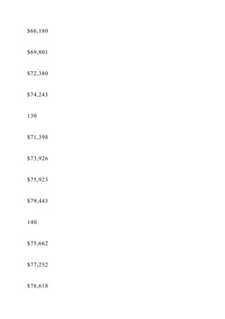
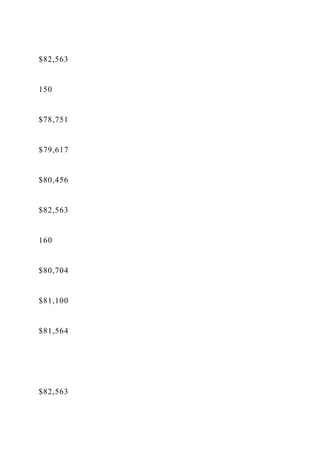
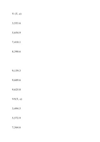
40, Λ3 = 50, Λ4 = 55 and Λ5 = 120 and
T = 1. The scaling factor was selected so that
5
Λ
i=1
i/a < .01 resulting in T ← aT = 2, 800.
We also
assume that the arrival rates are uniform over the horizon [0, T
], i.e., λj = Λj/T . In Table 10 we present
the expected revenues Vj(T, c), j = 1, . . . , 5 and V (T, c) for c
∈ {50, 100, 150, 200, 250}. The first row
is V5(c)
from Example 1. Notice that V5(c) ≤ V5(T, c). This is because
we here we are assuming uniform, rather
than

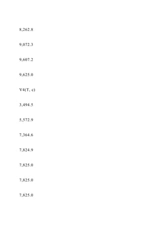
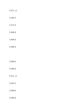
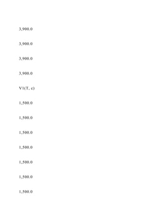
low-to-high arrivals. V (T, c) is even higher because we have
the flexibility of opening and closing fares
at
will. While the increase in expected revenues [V (T, c) − V5(T,
c)] due to the flexibility of opening and
closing
fares may be significant for some small values of c (it is 1.7%
for c = 50), attempting to go for this extra
revenue may invite strategic customers or third parties to
arbitrage the system. As such, it is not generally
recommended in practice.
c
50
100
150

200
250
300
350
V5(c)
3,426.8
5,441.3
7,188.7
8,159.1
8,909.1
9,563.9
9,625.0

V (T, c)
3,553.6
5,654.9
7,410.1
8,390.6
9,139.3
9,609.6
9,625.0
V5(T, c)
3,494.5
5,572.9
7,364.6

8,262.8
9,072.3
9,607.2
9,625.0
V4(T, c)
3,494.5
5,572.9
7,364.6
7,824.9
7,825.0
7,825.0
7,825.0

V3(T, c)
3,494.5
5,572.9
5,900.0
5,900.0
5,900.0
5,900.0
5,900.0
V2(T, c)
3,494.5
3,900.0
3,900.0

3,900.0
3,900.0
3,900.0
3,900.0
V1(T, c)
1,500.0
1,500.0
1,500.0
1,500.0
1,500.0
1,500.0
1,500.0

Table 10: Expected Revenues V (T, c) with uniform arrival rates
To obtain a continuous time formulation, we can use the same
logic that lead to (20) to obtain
∂Vj(t, x)
rjt − πjt∆Vj(t, x)
if (t, x) /
∈ Zj−1
=
(28)
∂t
∂Vj−1(t,x)
if (t, x) ∈ Z

∂t
j−1
with the same boundary conditions.
8.1
Mark-up and Mark-down Policies
We now go back to the broader pricing interpretation coupled
with the monotonic fare formulation (27).
In
many applications the price menu pjt, j = 1, . . . , n is time
invariant, but the associated sales rates πjt, j =
1, . . . , n are time varying. In addition, we will assume that
there is a price p0t such that π0t = 0 for all t.
This technicality helps with the formulation as a means of
turning off demand when the system runs out of
inventory. The case p1t ≥ p2t ≥ . . . ≥ pnt and π1t ≤ π2t ≤ . . . ≤
πnt is known as the mark-up problem,

while
the case p1t ≤ p2t ≤ . . . ≤ pnt and π1t ≥ π2t ≥ . . . ≥ πnt is
known as the mark-down problem. The former
model is relevant in Revenue Management while the second is
relevant in Retailing.
For the RM formulation, the problem can be viewed as
determining when to mark-up (switch from action
j to j − 1). The optimal mark-up times are random as they
depend on the evolution of sales under the
optimal policy. Suppose that the current state is (j, t, x), so the
last action was j, the time-to-go is t and the
inventory is x. We want to determine whether we should
continue using action j or switch to action j − 1.
We know that if x > yj−1(t), then we should keep action j and if
x ≤ yj−1(t) then we should close action
24

j. Let Zj = {(t, x) : x ≤ yj−1(t)}, then it is optimal to stop action
j upon first entering set Zj. Notice
that a mark-up occurs when the current inventory falls below a
curve, so low inventories trigger mark-
ups,
and mark-ups are triggered by sales. The retailing formulation
also has a threshold structure, but this time
a
mark-down is triggered by inventories that are high relative to a
curve, so the optimal timing of a mark-
down
is triggered by the absence of sales. Both the mark-up and the
mark-down problems can be studied from
the
point of view of stopping times. We refer the reader to Feng and
Gallego [9], [10], and Feng and Xiao
[11] and

reference therein for more on the markup and markdown
problems.
9
Acknowledgments
I acknowledge the feedback from my students and collaborators.
In particular, I would like to recognize
the
contributions and feedback from Anran Li, Lin Li, and Richard
Ratliff.
25
10
Appendix
Proof of Lemma 1. Notice that g(y) = G(y)P (X ≥ y) +
G(j)P (X = j), while g(y − 1) = G(y −
j≤y−1

1)P (X ≥ y) +
G(j)P (X = j). Taking the difference yields ∆g(y) = G(y)P (X ≥
y). Notice that
j≤y−1
r(y) = R(y)P (X < y) +
R(j)P (X = j) while r(y − 1) = R(y − 1)P (X < y) +
R(j)P (X = j).
j≥y
j≥y
Taking the difference we see that ∆r(y) = ∆R(y)P (X < y).
Proof of Proposition 1. Let G(y) = p1y, then V1(y) = g(y) =
EG(min(D1, y)), so ∆V1(y) = ∆g(y) =

p1P (D1 ≥ y). This establishes the first part of the Proposition.
To establish the second part of the
Proposition
we use the first part of Lemma 1 to show that p2E min(D2, c −
y) − p2E min(D2, c − y + 1) = −p2P (D2 >
c − y)
and the second part of the Lemma 1 to show that EV1(max(x −
D2, y)) − EV1(max(x − D2, y − 1)) =
∆V1(y)P (D2 > c−y). The second part of the Proposition then
follows from putting the two parts together.
To
see the first part, let r(y) = p2c−p2E max(c−D2, y), then ∆r(y) =
p2E min(D2, c−y)−p2E min(D2, c−y+1)
=
∆R(y)P (c − D2 < y) where R(y) = −p2y, so ∆r(y) = −p2P (c −
D2 < y) = −p2P (D2 > c − y). Now let
R(y) = V1(y), then ∆r(y) = ∆V1(y)P (c − D2 < y) = ∆V1(y)P
(D2 > c − y) completing the proof.

Proof of Lemma 2: We will prove the above result by induction
on j. The result is true for j = 1 since
∆V1(y) = p1P (D1 ≥ y) is decreasing in y and clearly ∆V1(y) =
p1P (D1 ≥ y) ≥ ∆V0(y) = 0. Assume that
the
result is true for Vj−1. It follows from the dynamic
programming equation (8) that
Vj(x) = max {Wj (y, x))} ,
y≤x
where for any y ≤ x,
Wj(y, x) = E [pj min {Dj, x − y}] + E [Vj−1 (max {x − Dj, y})]
A little work reveals that for y ∈ {1, . . . , x}
∆Wj(y, x) = Wj(y, x) − Wj(y − 1, x) = [∆Vj−1(y) − pj] P (Dj > x
− y).
Since ∆Vj−1(y) is decreasing in y (this is the inductive
hypothesis), we see that Wj(y, x) ≥ Wj(y − 1, x)

if ∆Vj−1(y) > pj and Wj(y, x) ≤ Wj(y − 1, x) if ∆Vj−1(y) ≤ pj.
Consider the expression
yj−1 = max{y ∈ N : ∆Vj−1(y) > pj}
(29)
where the definition of ∆Vj(y) is extend to y = 0 for all j by
setting ∆Vj(0) = p1. If yj−1 ≤ x then
Vj(x) = max Wj(y, x) = Wj(yj−1, x)
y≤x
On the other hand, if x < yj−1 then
Vj(x) = max Wj(y, x) = Wj(x, x).
y≤x
In summary,

Vj(x)
=
Wj(min(x, yj−1), x)
V
=
j−1(x),
if x ≤ yj−1
E [pj min {Dj, x − yj−1}] + E [Vj−1 (max {x − Dj, yj−1})]
if x > yj−1
26
Computing ∆Vj(x) = Vj(x) − Vj(x − 1) for x ∈ N results in:
∆V

∆V
j−1(x),
if x ≤ yj−1
j (x)
=
(30)
E min(pj, ∆Vj−1(x − Dj))
if x > yj−1
We will now use this result to show that ∆Vj(x) is itself
decreasing in x. Since ∆Vj(x) = ∆Vj−1(x) for
x ≤ yj−1 and ∆Vj−1(x) is decreasing in x we only need to worry
about the case x > yj−1.
However, in this case

∆Vj(x) = E min(pj, ∆Vj−1(x − Dj))
is decreasing in x since ∆Vj−1(x) is itself decreasing in x.
We now show that ∆Vj(x) ≥ ∆Vj−1(x). For x > yj−1 we have
min(pj, ∆Vj−1(x−Dj)) ≥ min(pj, ∆Vj−1(x))
=
∆Vj−1(x) where the inequality follows since ∆Vj−1(x) is
decreasing in x and the equality since x > yj−1.
Tak-
ing expectations we see that ∆Vj(x) ≥ ∆Vj−1(x) on x > yj−1
while ∆Vj(x) = ∆Vj−1(x) on x ≤ yj−1.
Proof of Proposition 2. We first show that ∆Vj+1(x) = ∆Vj(x)
for x = 1, . . . , yj. This follows since
Vj+1(x) = Wj+1(x, x) = Vj(x) in this range as no capacity is
made available for fare pj+1 when x ≤ yj.
For
x > yj

Vj+1(x)
=
pj+1E min(x − yj, Dj+1) + EVj(max(x − Dj+1, yj)
x−yj
=
pj+1
P r(Dj+1 ≥ k) + Vj(yj)P r(Dj+1 > x − yj)
k=1
x−yj
+
Vj(x − k)P r(Dj+1 = k).
k=0

Consequently, for x > yj
x−yj −1
∆Vj+1(x) = pj+1P r(Dj+1 ≥ x − yj) +
∆Vj(x − k)P r(Dj+1 = k)
(31)
k=0
follows from Vj(x − 1) = Vj(yk) for x = yj + 1. Since pj+1 <
∆Vj(y) for y ≤ yj, we can write ∆Vj+1(x) =
∞
min(p
k=0
j+1, ∆Vj (x − k))P (Dj+1 = k) = E min(pj+1, ∆Vj (x − Dj+1)).
Proof of Proposition 3. Since Πn(c, k) is the difference of a

concave and a linear function, Πn(c, k) it is
itself concave. The marginal value of adding the cth unit of
capacity is ∆Vn(c) − k so the cth unit increase
profits as long as ∆Vn(c) > k. Therefore, the smallest optimal
capacity is given by c(k). (Notice that c(k)
+ 1
may be also optimal if ∆Vn(c(k) + 1) = k.) c(k) is decreasing in
k since ∆Vn(c) is decreasing in c.
Suppose
that k = pj+1. To establish c(pj+1) = yj it is enough to show that
that ∆Vn(yj) > pj+1 ≥ ∆Vn(yj + 1). By
definition yj = max{y ∈ N : ∆Vj(y) > pj+1} so ∆Vj(yj) > pj+1 ≥
∆Vj(yj + 1). Since it is optimal to
protect
up to yj units of capacity for sale at fares j, j − 1, . . . , 1, it
follows that Vn(c) = Vj(c) for all c ≤ yj, and
consequently ∆Vn(yj) = ∆Vj(yj) > pj+1. Now ∆Vn(yj + 1) can
be written as a convex combination of

pj+1
and ∆Vj(yj + 1) ≤ pj+1 which implies that ∆Vn(yj + 1) ≤ pj+1,
completing the proof.
Proof of Lemma 3: We will first show part that ∆Vj(t, x) is
decreasing in x which is equivalent to
showing
that 2Vj(t, x) ≥ Vj(t, x + 1) + Vj(t, x − 1)] for all x ≥ 1. Let A
be an optimal admission control rule starting
from state (t, x + 1) and let B be an optimal admission control
rule starting from (t, x − 1). These
admission
control rules are mappings from the state space to subsets Sk =
{1, . . . , k}, k = 0, 1, . . . , j where S0 = ∅
is
the optimal control whenever a system runs out of inventory.
Consider four systems: two starting from
state

(t, x), using control rules A and B , respectively, and one each
starting from (t, x + 1) and (t, x − 1), using
control rule A and B, respectively. Our goal is to specify
heuristic control rules A and B that together
make
the expected revenues of the two systems starting with (t, x) at
least as large as the expected revenues
from
the systems starting at (t, x + 1) and (t, x − 1). This will imply
that 2Vj(t, x) ≥ Vj(t, x + 1) + Vj(t, x − 1).
27
We will use the control rules A = A ∩ B and B = A ∪ B until
the first time, if ever, the remaining
inventory of the system (t, x) controlled by A is equal to the
remaining inventory of the system (t, x + 1)
controlled by A. This will happen the first time, if ever, there is
a sale under A and not under A , i.e., a

sale
under A but not under B. Let t be the first time this happens, if
it happens before the end of the horizon,
and set t = 0 otherwise. If t > 0 then we apply policy A = A and
B = B over s ∈ [0, t ). We claim that the
expected revenue from the two systems starting with (t, x) is the
same as the expected revenue from the
other
two systems. This is because the sales and revenues up to, but
before t , are the same in the two systems.
At t sales occur only for the system (t, x) controlled by B and
the system (t, x + 1) controlled by A and the
revenues from the two sales are identical. After the sales at t ,
the inventory of the system (t, x) controlled
by
A becomes identical to the inventory of the system (t, x + 1)
controlled by A while the inventory of the
system

(t, x) controlled by B becomes identical to the inventory of the
system (t, x − 1) controlled by B. Since the
policy switches to A = A and B = B then sales and revenues are
the same over [0, t ). If t = 0 then the
sales of the two systems are the same during the entire horizon.
It remains to verify that inventories don’t become negative.
Prior to time t the systems remain balance
in the sense that system (t, x) governed by A always has one
unit of inventory less than system (t, x + 1)
governed by A and system (t, x) governed by B has one more
unit of inventory than system (t, x − 1)
governed
by B. Thus the only two systems that could potential run out of
inventory before t are A and B.
Since sales under A = A∩B are more restricted than sales under

B, the inventory of system (t, x) governed
by A will always be at least one unit since at most x − 1 units of
sale are allowed under B. Therefore the
only way the system can run out of inventory is if system (t, x −
1) runs out of inventory under B before t .
However, in this case sales would stop under systems A and B,
while sales will continue under B = A
and A
so revenues will continue to be the same until the first sale
under A at which point we reached t . This
shows
that even if the system (t, x − 1) runs out of inventory under B
the two systems continue to have the same
revenues over the entire horizon. Consequently 2∆Vj(t, x) ≥
Vj(t, x + 1) + Vj(t, x − 1) for all x ≥ 1.
To show that ∆Vj(t, x) is increasing in j it is enough to show
that

Vj(t, x) + Vj−1(t, x − 1) ≥ Vj(t, x − 1) + Vj−1(t, x).
To do this we again use a sample path argument. Let A be an
optimal admission control rule for the
system
(j, t, x − 1) and B be an admission control rule for the system (j
− 1, t, x) Let A and B be heuristic
admission
rules applied, respectively, to the systems (j, t, x) and (j −1, t,
x−1). Our goal is to exhibit heuristics A
and B
such that when applied to the systems (j, t, x) and (j −1, t, x−1)
they generate as much revenue as the
applying
A to (j, t, x − 1) and B to (j − 1, t, x). This will imply that Vj(t,
x) + Vj−1(t, x − 1) ≥ Vj(t, x − 1) + Vj−1(t,
x).
Let A = A ∪ B and B = A ∩ B and let t be the first time there is
a sale under A ∪ B without a

corresponding sale in A, so there is a sale under B but not under
A. If t = 0 then the revenues of the sets
of two systems are equal. If t > 0 switch at that point to the
policy A = A and B = B. Then sales and
revenues under both sets of two systems are equal up to t . At t
there are sales for the system (j, t, x) and
(j − 1, t, x − 1) that generate the same revenues. Moreover, the
inventories of the two sets of two systems
have
the same inventories immediately after the sale at t . Since the
policy then switches to A = A and B = B
then sales and revenues are the same for the two set of systems
over s ∈ [0, t ). The only system in danger
to
run out of inventory is system (j, t, x) under A = A ∪ B, but
that system has the same number of sales as
the

system (j, t, x − 1) under A up to t . Therefore the system (j, t,
x) has at least one unit of inventory up to t .
To show that ∆Vj(t, x) is increasing in t it is enough to show
that
Vj(t, x) + Vj(t − 1, x − 1) ≥ Vj(t, x − 1) + Vj(t − 1, x).
To do this we again use a sample path argument. Let A be an
optimal admission control rule for the
system
(t, x − 1) and B be an optimal admission control rule for the
system (t − 1, x) Let A and B be heuristic
admission rules applied, respectively, to the systems (t, x) and
(t − 1, x − 1). Our goal is to exhibit
heuristics
A and B such that when applied to the systems (t, x) and (t − 1,
x − 1) they generate as much revenue as
the
applying A to (t, x−1) and B to (t−1, x). This will imply that

Vj(t, x)+Vj(t−1, x−1) ≥ Vj(t, x−1)+Vj(t−1,
x).
Let A = A ∪ B and B = A ∩ B and let t be the first time there is
a sale under A without a corresponding
28
sale in A, so there is a sale under B but not under A. If t = 0
then the revenues of the sets of two systems
are
equal. If t > 0 switch at that point to the policy A = A and B =
B. Then sales and revenues under both
sets of two systems are equal up to t . At t there are sales for the
system (t, x) and (t − 1, x) that generate
the
same revenues. Moreover, the inventories of the two sets of two
systems have the same inventories
immediately

after the sale at t . Since the policy then switches to A = A and
B = B then sales and revenues are the
same for the two set of systems over s ∈ [0, t ). The only
system in danger to run out of inventory is
system
(t − 1, x − 1) under B = A ∪ B, but that system has the same
number of sales as the system (t − 1, x) under
B up to t . Therefore the system (t − 1, x − 1) has at least one
unit of inventory up to t .
Proof of Lemma 4. We will first show that aj(t, x) can also be
characterized as aj(t, x) = max{k ≤
j : pk ≥ ∆Vk(t − 1, x)}. The result will then follow from Lemma
3. First notice that if aj(t, x) = k < j
then Vi(t, x) = Vk(t, x) for all i ∈ {k, . . . , j}. Moreover, aj(t,
x) = k < j implies that Wk(t, x) > Wk+1(t,
x).
Consequently 0 > Wk+1(t, x)−Wk(t, x) = (pk+1 −∆Vk+1(t−1,
x))λk+1, so pk+1 < ∆Vk+1(t−1, x).

Conversely,
if pk ≥ ∆Vk(t − 1, x) then Wk(t, x) − Wk−1(t, x) ≥ (pk − ∆Vk(t
− 1, x))λk ≥ 0 so Wk(t, x) ≥ Wk−1(t, x).
With
the new characterization we now turn to the monotonicity of
aj(t, x) = max{k ≤ j : pk ≥ ∆Vk(t − 1, x)}.
The monotonicity with respect to j is obvious because it
expands the set over which we are maximizing.
To see the monotonicity with respect to t, notice that ∆Vk(t, x)
≥ ∆Vk(t − 1, x) so k is excluded from
the set whenever ∆Vk(t − 1, x) ≤ pk < ∆Vk(t, x). To see the
monotonicity with respect to x, notice that
∆Vk(t − 1, x + 1) ≤ ∆Vk(t, x) ≤ pk implies that k contributes
positively at state (t − 1, x + 1) whenever it
contributes at (t − 1, x).
29

11
Terminology
Item
Description
c
capacity
p
price
s
salvage value on excess capacity after the arrival of full-fare
demand (e.g. last-
minute travel specials).

x
remaining capacity, i.e. x ∈ {0, 1, ..., c}
E
expected value operator
j
fare class identifier where price decreases with increasing class
index, i.e. p1 ≥
p2 ≥ .. ≥ pj
p
demand weighted average fare class price
j
D
fare class demand

y
protection level for a fare class
ya
protection level obtained using EM SRa heuristic
yb
protection level obtained using EM SRb heuristic
W (y, c)
revenue given protection level y and capacity c
r
ratio of discount to full-fare price
F
cumulative density function (CDF) of continuous demand

F −1
inverse density function of continuous demand
b
booking limit for sales of discount fares
Vj(x)
optimal expected revenue for classes {1, 2, ..., j} from capacity
x
ρ
penalty cost for each unit of full-fare demand that is rejected
sj
observed sales for fare j in Monte Carlo simulation
Sk
Set of highest k fares {1, . . . , k}

a(t, x)
highest opened fare class at state (t, x)
Zj
the stopping set for fare j (where it is optimal to close down
fare j upon entering
set Zj)
λjt
arrival rate of fare j demand at time-to-go t
Λjt
expected demand for fare j over [0, t].
Table 11: Summary of Terminology and Notation Used
References

[1] Bathia, A. V. and S. C. Prakesh (1973) “Optimal Allocation
of Seats by Fare,” Presentation by TWA
Airlines to AGIFORS Reservation Study Group.
[2] Belobaba, P. P. (1987) “Airline Yield Management An
Overview of Seat Inventory Control,”
Transporta-
tion Science, 21, 63–73.
[3] Belobaba, P. P. (1989) “Application of a Probabilistic
Decision Model to Airline Seat Inventory
Control,”
Operations Research, 37, 183–197.
[4] Brumelle, S. L., J. I. McGill, T. H. Oum, M. W. Tretheway
and K. Sawaki (1990) “Allocation of
Airline
Seats Between Stochastically Dependent Demands,”
Transporation Science, 24, 183-192.

[5] Brumelle, S. L. and J. I. McGill (1993) “Airline Seat
Allocation with Multiple Nested Fare Classes,”
Operations Research, 41, 127-137.
30
[6] Curry, R. E. (1990) “Optimal Airline Seat Allocation with
Fare Nested by Origins and Destinations,”
Transportation Science, 24, 193–204.
[7] Diwan, S. (2010) “Performance of Dynamic Programming
Methods in Airline Revenue Management.”
M.S. Dissertation MIT. Cambridge, MA.
[8] Chandler, S. and Ja, S. (2007) Revenue Opportunity
Modeling at American Airlines. AGIFORS
Reser-
vations and Yield Management Study Group Annual Meeting
Proceedings; Jeju, Korea.
[9] Feng, Y. and G. Gallego (1995) “Optimal Starting Times of

End-of-Season Sales and Optimal
Stopping
Times for Promotional Fares,” 41, 1371-1391.
[10] Feng, Y. and G. Gallego (2000) “Perishable asset revenue
management with Markovian time-
dependent
demand intensities,” Management Science, 46(7): 941-956.
[11] Feng, Y. and B. Xiao (2000) “Optimal policies of yield
management with multiple predetermined
prices,”
Operations Research, 48(2): 332-343.
[12] Gallego, G., S. Kou and Phillips, R. (2008) “Revenue
Management of Callable Products,”
Management
Science, 54(3): 550564.

[13] Lee. C. T. and M. Hersh. (1993) “A Model for Dynamic
Airline Seat Inventory Control with
Multiple
Seat Bookings,” Transportation Science, 27, 252–265.
[14] Littlewood, K. (1972) “Forecasting and Control of
Passenger Bookings.” 12th AGIFORS
Proceedings:
Nathanya, Israel, reprinted in Journal of Revenue and Pricing
Management, 4(2): 111-123.
[15] Pfeifer, P. E. (1989) “The Airline Discount Fare Allocation
Problem,” Decision Science, 20, 149–
157.
[16] Ratliff, R. (2005) “Revenue Management Demand
Distributions”, Presentation at AGIFORS
Reservations
and Yield Management Study Group Meeting, Cape Town,
South Africa, May 2005.
[17] Richter, H. (1982) “The Differential Revenue Method to

Determine Optimal Seat Allotments by Fare
Type,” In Proceedings 22nd AGIFORS Symposium 339-362.
[18] Robinson, L.W. (1995) “Optimal and Approximate Control
Policies for Airline Booking With
Sequential
Nonmonotonic Fare Classes,” Operations Research, 43, 252-
263.
[19] Simpson, R. (1985) “Theoretical Concepts for
Capacity/Yield Management,” In Proceedings 25th
AGI-
FORS Symposium 281-293.
[20] Talluri, K and G. van Ryzin (2004) “The Theory and
Practice of Revenue Management,” Springer
Sci-
ence+Business Media, New York, USA, pg. 42.
[21] Tematha, C., S. Polt, and and L. Suhi. (2010) “On the
robustness of the network-based revenue

oppor-
tunity model,” Journal of Revenue and Pricing Management ,
Vol. 9, 4, 341355.
[22] Wollmer, R. D. (1992) “An Airline Seat Management
Model for a Single Leg Route When Lower
Fare
Classes Book First,” Operations Research, 40, 26-37.
[23] Zhao, W. and Y-S Zheng (2001) “A Dynamic Model for
Airline Seat Allocation with Passenger
Diversion
and No-Shows,” Transportation Science,35: 80-98.
31
Probability

and Dynamic Programming
Review
for
Dynamic Pricing and Revenue
Management
Probability Review
• Poisson:
http://en.wikipedia.org/wiki/Poisson_random_variable
–
Read Sections: 1, 2, 3,4
• Compound Poisson:
http://en.wikipedia.org/wiki/Compound_Poisson_distribution
• Poisson Process: http://en.wikipedia.org/wiki/Poisson_process

• Compound Poisson Process:
http://en.wikipedia.org/wiki/Compound_Poisson_process
• Normal: http://en.wikipedia.org/wiki/Normal_random_variable
–
Read Sections 1,2.1,2.2,3,1,3.2,3.3
• Brownian Motion:
http://en.wikipedia.org/wiki/Wiener_process
–
Read sections 1, 2.
DP AS AN OPTIMIZATION METHODOLOGY
• Basic optimization problem
min g( u)

u∈ U
where u is the optimization/decision variable, g( u) is the cost
function, and U is the constraint set
• Categories of problems:
− Discrete ( U is finite) or continuous
− Linear ( g is linear and U is polyhedral) or nonlinear
− Stochastic or deterministic: In stochastic problems the cost
involves a stochastic parameter
w, which is averaged, i.e., it has the form g( u) = Ew G( u, w)
where w is a random parameter.
• DP can deal with complex stochastic problems where
information about w becomes available in stages,
and the decisions are also made in stages and make use of this
information.
INVENTORY CONTROL EXAMPLE

w
Demand at Period k
k
Stock at Period k
Stock at Period k + 1
Inventory
xk
S y s t e m
xk + 1 = xk + uk - wk
Stock Ordered at
Period k
Co s t o f P e rio d k
u k

c uk + r (xk + uk - wk)
• Discrete-time system
xk+1 = fk( xk, uk, wk) = xk + uk − wk
• Cost function that is additive over time N − 1
E
gN ( xN ) +
gk( xk, uk, wk)
k=0
N − 1
= E
cuk + r( xk + uk − wk) k=0

• Optimization over policies: Rules/functions uk =
µk( xk) that map states to controls BASIC STRUCTURE OF
STOCHASTIC DP
• Discrete-time system
xk+1 = fk( xk, uk, wk) , k = 0 , 1 , . . . , N − 1
− k: Discrete time
− xk: State; summarizes past information that is relevant for
future optimization
− uk: Control; decision to be selected at time k from a given set
− wk: Random parameter (also called distur-bance or noise
depending on the context)
− N: Horizon or number of times control is applied
• Cost function that is additive over time N − 1
E

gN ( xN ) +
gk( xk, uk, wk)
k=0
BASIC PROBLEM
• System xk+1 = fk( xk, uk, wk), k = 0 , . . . , N − 1
• Control constraints uk ∈ U( xk)
• Probability distribution Pk( · | xk, uk) of wk
• Policies π = {µ 0 , . . . , µN− 1 }, where µk maps states xk
into controls uk = µk( xk) and is such that
µk( xk) ∈ Uk( xk) for all xk
• Expected cost of π starting at x 0 is N − 1
Jπ( x 0) = E gN ( xN ) +
gk( xk, µk( xk) , wk) k=0

• Optimal cost function
J ∗ ( x 0) = min Jπ( x 0) π
• Optimal policy π∗ is one that satisfies Jπ∗ ( x 0) = J∗ ( x 0)
PRINCIPLE OF OPTIMALITY
• Let π∗ = {µ∗ 0 , µ∗ 1 , . . . , µ∗ N− 1 } be an optimal policy
• Consider the “tail subproblem” whereby we are at xi at time i
and wish to minimize the “cost-to-go”
from time i to time N
N − 1
E
gN ( xN ) +
gk xk, µk( xk) , wk
k= i
and the “tail policy” {µ∗ , µ∗

i
i+1 , . . . , µ∗
N − 1 }
xi
Tail Subproblem
0
i
N
• Principle of optimality: The tail policy is optimal for the tail
subproblem
• DP first solves ALL tail subroblems of final stage
• At the generic step, it solves ALL tail subproblems of a given

time length, using the solution of the tail
subproblems of shorter time length
DP ALGORITHM
• Start with
JN ( xN ) = gN ( xN ) , and go backwards using
Jk( xk) =
min
E gk( xk, uk, wk)
uk∈ Uk( xk) wk
+ Jk+1 fk( xk, uk, wk) , k = 0 , 1 , . . . , N − 1 .
• Then J 0( x 0), generated at the last step, is equal to the
optimal cost J ∗ ( x 0). Also, the policy π∗ =
{µ∗ 0 , . . . , µ∗ N− 1 }
where µ∗ ( x

k
k) minimizes in the right side above for
each xk and k, is optimal.
• Justification: Proof by induction that Jk( xk) is equal to J ∗ ( x
k
k), defined as the optimal cost of
the tail subproblem that starts at time k at state xk.
• Note that ALL the tail subproblems are solved in addition to
the original problem, and the inten-sive
computational requirements.
DETERMINISTIC FINITE-STATE PROBLEM
Terminal Arcs
with Cost Equal

to Terminal Cost
. . .
t
Artificial Terminal
. . .
N o d e
Initial State
s
. . .
Stage 0
Stage 1
Stage 2

. . . Stage N - 1
Stage N
• States < == > Nodes
• Controls < == > Arcs
• Control sequences (open-loop) < == > paths from initial state
to terminal states
• ak : Cost of transition from state i ∈ Sk to state ij
j ∈ Sk+1 at time k (view it as “length” of the arc)
• aN : Terminal cost of state i ∈ S
it
N
• Cost of control sequence < == > Cost of the cor

responding path (view it as “length” of the path) BACKWARD
AND FORWARD DP ALGORITHMS
• DP algorithm:
JN ( i) = aN , i ∈ S
it
N ,
Jk( i) = min ak + Jk+1( j) , i ∈ Sk, k = 0 , . . . , N − 1 .
j∈ S
ij
k+1
The optimal cost is J 0( s) and is equal to the length of the
shortest path from s to t.
• Observation: An optimal path s → t is also an optimal path t
→ s in a “reverse” shortest path problem
where the direction of each arc is reversed and its length is left

unchanged.
• Forward DP algorithm (= backward DP algorithm for the
reverse problem):
˜
JN ( j) = a 0 , j ∈ S
sj
1 ,
˜
Jk( j) = min aN−k + ˜
Jk+1( i) , j ∈ SN−k+1
i∈ S
ij
N−k

The optimal cost is ˜
J 0( t) = min i∈ S
aN + ˜
J
N
it
1( i) .
• View ˜
Jk( j) as optimal cost-to-arrive to state j from initial state s.
A NOTE ON FORWARD DP ALGORITHMS
• There is no forward DP algorithm for stochastic problems.
• Mathematically, for stochastic problems, we cannot restrict

ourselves to open-loop sequences, so the
shortest path viewpoint fails.
• Conceptually, in the presence of uncertainty, the concept of
“optimal-cost-to-arrive” at a state xk does
not make sense. The reason is that it may be impossible to
guarantee (with prob. 1) that any given state
can be reached.
• By contrast, even in stochastic problems, the concept of
“optimal cost-to-go” from any state xk makes
clear sense.
GENERIC SHORTEST PATH PROBLEMS
• { 1 , 2 , . . . , N, t}: nodes of a graph ( t: the desti-nation)
• aij: cost of moving from node i to node j
• Find a shortest (minimum cost) path from each node i to node
t
• Assumption: All cycles have nonnegative length.
Then an optimal path need not take more than N

moves
• We formulate the problem as one where we require exactly N
moves but allow degenerate moves from a
node i to itself with cost aii = 0.
Jk( i) = optimal cost of getting from i to t in N −k moves.
J 0( i): Cost of the optimal path from i to t.
• DP algorithm:
Jk( i) = min
aij+ Jk+1( j) ,
k = 0 , 1 , . . . , N − 2 , j=1 ,...,N
with JN− 1( i) = ait, i = 1 , 2 , . . . , N.
EXAMPLE

State i
Destination
5
5
3
3
3
3
2
3
4
7
5

0 . 5
0
1
2
3
4
Stage k
(a)
(b)
JN− 1( i) = ait,
i = 1 , 2 , . . . , N,

Jk( i) = min
aij+ Jk+1( j) ,
k = 0 , 1 , . . . , N − 2 .
j=1 ,...,N
Document Outline
Probability and Dynamic ProgrammingReview
Probability Review
Probability and Dynamic ProgrammingReviewProbability
Review
IEOR 4601 Homework 1: Due Wednesday, February 6
1. A coffee shop gets a daily allocation of 100 bagels.
The bagels can be either sold
individually at $0.90 each or can be used later in the day for

sandwiches. Each bagel
sold as a sandwich provides a revenue of $1.50 independent of
the other ingredients.
a) Suppose that demand for bagel sandwiches is estimated to be
Poisson with param-
eter 100. How many bagels would you reserve for sandwiches?
b) Compare the expected revenue of the solution of part a) to
the expected revenue
of the heuristic that does not reserve capacity for sandwiches
assuming that the
demand for individual bagels is Poisson with parameter 150?
c) Answer part a) if the demand for bagel sandwiches is normal
with mean 100 and
standard deviation 20.
2. Problem 2 in the textbook (page 173)

3. Problem 3 in the textbook (page 173)
[Hint: For problem 2 and 3, you might want to consider the
NORMINV() function in
Excel.]
4. Suppose capacity is 120 seats and there are four fares. The
demand distributions for
the different fares are given in the the following table.
Class
Fare
Demand Distribution
1
$200
Poisson(25)
2

$175
Poisson(30)
3
$165
Poisson(29)
4
$130
Poisson(30)
Determine the optimal protection levels. [Hints: The sum of
independent Poisson ran-
dom variables is Poisson with the obvious choice of parameter
to make the means match.

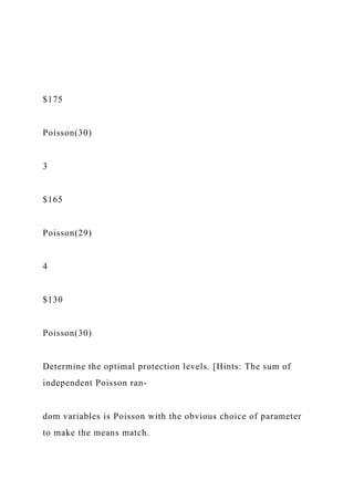
If D is Poisson with parameter λ then P (D = k + 1) = P (D =
k)λ/(k + 1) for any non-
negative integer k. You might want to investigate the
POISSON() function in Excel.]
5. Consider a parking lot in a community near Manhattan. The
parking lot has 100 parking
spaces. The parking lot attracts both commuters and daily
parkers. The parking lot
manager knows that he can fill the lot with commuters at a
monthly fee of $180 each. The
parking lot manager has conducted a study and has found that
the expected monthly
revenue from x parking spaces dedicated to daily parkers is
approximated well by the
quadratic function R(x) = 300x − 1.5x2 over the range x ∈ {0,
1, . . . , 100}.
Note:

Assume for the purpose of the analysis that parking slots rented
to commuters cannot
be used for daily parkers even if some commuter do not always
use their slots.
a) What would the expected monthly revenue of the parking lot
be if all the capacity
is allocated to commuters?
1
b) What would the expected monthly revenue of the parking lot
be if all the capacity
is allocated to daily parkers?
c) How many units should the parking manager allocate to daily
parkers and how
many to commuters?

d) What is the expected revenue under the optimal allocation
policy?
6. A fashion retailer has decided to remove a certain item of
clothing from the racks in
one week to make room for a new item. There are currently 80
units of the item and
the current sale price is $150 per unit. Consider the following
three strategies assuming
that any units remaining at the end of the week can be sold to a
jobber at $30 per unit.
a) Keep the current price. Find the expected revenue under this
strategy under the
assumption that demand at the current price is Poisson with
parameter 50.
b) Lower the price to $90 per unit. Find the expected revenue
under this strategy

under the assumption that demand at $90 is Poisson with
parameter 120.
c) Keep the price at $150 but e-mail a 40% discount coupon for
the item to a popula-
tion of price sensitive customers that would not buy the item at
$150. The coupon
is valid only for the first day and does not affect the demand for
the item at $150.
Compute the expected revenue under this strategy assuming that
the you can con-
trol the number of coupons e-mailed so that demand from the
coupon population
is Poisson with parameter x for values of x in the set {0, 5, 10,
15, 20, 25, 30, 35}. In
your calculations assume that demand from coupon holders
arrives before demand
from customers willing to pay the full price. Assume also that

you cannot deny
capacity to a coupon holder as long as capacity is available (so
capacity cannot be
protected for customers willing to pay the full price). What
value of x would you
select? You can assume, as in parts a) and b) that any leftover
units are sold to
the jobber at $30 per unit.
2

Dynamic Pricing andRevenue ManagementIEOR 4601 Spring .docx

More Related Content

Similar to Dynamic Pricing andRevenue ManagementIEOR 4601 Spring .docx

More from jacksnathalie

Recently uploaded

Dynamic Pricing andRevenue ManagementIEOR 4601 Spring .docx