Download to read offline
![M. Rezaee Manesh et al./ Journal of Soft Computing in Civil Engineering 4-4 (2020) 98-111 99
1. Introduction
Swarm intelligence (SI) is the collective behavior of decentralized systems consisting of many
individuals who coordinate their activities using self-organization [1]. The SI systems are
inspired by biological systems that are usually composed of a population of simple agents
interacting with each other and globally with their environment. Ant colonies [2], bird flocks
[3,4], honey bee colonies [5,6], and fish schools [7,8] are examples of natural SI systems. Based
on the systems, several optimization algorithms such as ant colony, artificial honey bee colony,
and particle swarm optimization (PSO) algorithms have been developed. PSO is a computational
method based on a powerful population that is capable of solving the problem using the
population of candidate solutions. To improve the candidate solution, PSO frequently moves the
candidates using simple mathematical equations in a search space [9]. Since the introduction by
Kennedy and Eberhart (1995) [10] and Eberhart and Kennedy (1995) [11], the PSO algorithm
has been successfully used in various fields of civil engineering.
The optimization methods and algorithms are divided into two categories: exact algorithms and
approximate algorithms. Exact algorithms can accurately find the optimal solution, but they do
not work in hard optimization problems, and the solving time in these problems increases
exponentially. Approximate algorithms can find good (quasi-optimal) solutions to difficult
optimization problems in the short solving time. Approximate algorithms are also divided into
two categories: heuristic and meta-heuristic algorithms. The two major problems with heuristic
algorithms are (1) falling in local optima, and (2) inability to be applied to different problems.
The meta-heuristic algorithms have been proposed to solve the problems of heuristic algorithms.
The meta-heuristic algorithms are one of the approximate optimization algorithms that have the
mechanism to exit local optima and can be used in a wide range of problems. In recent decades,
various categories of this type of algorithm have been developed. Over the past few years, PSO
has been widely used in various aspects of geotechnical engineering such as slope stability
analysis, pile and foundation engineering, rock and soil mechanics, tunneling, and underground
space design [12].
2. Particle swarm optimization algorithm
In many optimization problems, especially the big ones, choosing the best solution through the
global search, though not being impossible, is very difficult. The goal of the optimization
problem is to reduce the search time. Heuristic methods are good solutions for finding the
optimal solution, but they do not guarantee to find the optimal solution. Today, however, as the
problems become bigger, the popularity of heuristic and meta-heuristic methods has considerably
grown.
Particle swarm optimization (PSO) is one of the meta-heuristic optimization techniques that
work based on the population. The original idea for the method was first proposed in 1995 by
Kennedy and Eberhart [10] which was inspired by the collective behavior of fish and birds for
finding the food. A group of birds and fish look for food in random space, and there is only one
piece of food, and none of the birds knows the location of the food and only knows the distance](https://image.slidesharecdn.com/sccevolume4issue4pages98-111-250515104151-99302d6c/85/Dual-Target-Optimization-of-Two-Dimensional-Truss-Using-Cost-Efficiency-and-Structural-Reliability-Sufficiency-2-320.jpg)
![100 M. Rezaee Manesh et al./ Journal of Soft Computing in Civil Engineering 4-4 (2020) 98-111
to the food. One of the best strategies is to follow a bird that is closest to the food. This view is
the main strategy of the algorithm.
In this method, each bird has a possible solution in the problem space called a particle. Each
particle has a fitness value that is calculated by the problem. The particle that is closest to the
solution has the highest fitness. This algorithm has a continuous nature and has been proven to
be efficient in numerous applications [13].
This algorithm is one of the population-based parallel search algorithms that start with a group of
random solutions (particles) and then continues to search for finding the optimal solution in the
problem space by updating the position of the particles. Each particle is denoted in the
multidimensional mode (depending on the type of problem) by two vectors Xid and Vid, which
represent the position and velocity in dimension d of particle i, respectively. At each stage of the
population movement, the position of each particle is updated by two best values. The first value
is the best experience ever gained by a particle and is represented by p_best. The second value is
the best experience gained among all the particles and is shown by g_best. In each iteration, after
finding these two values, the algorithm updates the new velocity and position of the particle-
based on Equations (1) and (2).
𝑣𝑖𝑑(𝑡 + 1) = 𝑤. 𝑣𝑖𝑑(𝑡) + 𝑐1. 𝑟𝑎𝑛𝑑1(𝑝_𝑏𝑒𝑠𝑡𝑖𝑑 (𝑡) − 𝑥𝑖𝑑(𝑡)) + 𝑐2. 𝑟𝑎𝑛𝑑2 (𝑔 _𝑏𝑒𝑠𝑡𝑖𝑑(𝑡) – 𝑥𝑖𝑑(𝑡)) (1)
xid(t + 1) = xid(t) + vid(t + 1) (2)
In Equation (1), w is the inertia weight factor, which is usually in the range [0-1]. C1 and C2 are
the learning or acceleration factors, which are selected in the range [0-2], which, in most cases,
are set to 1.49 or 2. rand1 and rand2 are also two random numbers in the range [0-1]. Also, the
final value of each particle's velocity to prevent algorithm divergence is limited to one range.
𝑣𝑖𝑑 ∈ [−𝑣𝑚𝑎𝑥 . 𝑣𝑚𝑎𝑥] is the termination condition of the convergence algorithm to a certain
extent or to stop after a certain number of iterations. Equation (2) also updates the current
position vector of the particle according to its new velocity.
The right side of Equation (1) consists of three parts; the first part is a factor of the current
velocity of the particle, the second part is used for changing the velocity and rotation of the
particle towards the best personal experience, and the third part is used for changing the velocity
and rotation of the particle towards the best group experience.
The optimization of the particle swarm without the first part of Equation (1) will be a process in
which the search space is gradually reduced and the local search is formed around the best
particle. In contrast, the first part of Equation (1) will cause the particles to move in their normal
direction to reach the wall of the search area and perform some sort of global search. By
combining the two factors, it was attempted to strike a balance between local and global search.
To better strike such balance, w was first proposed in [14], which specifies the movement factor
in the global search. The parameters c1 and c2 also specify the movement factor in local search.](https://image.slidesharecdn.com/sccevolume4issue4pages98-111-250515104151-99302d6c/85/Dual-Target-Optimization-of-Two-Dimensional-Truss-Using-Cost-Efficiency-and-Structural-Reliability-Sufficiency-3-320.jpg)
![M. Rezaee Manesh et al./ Journal of Soft Computing in Civil Engineering 4-4 (2020) 98-111 101
Start
Initialize
PSO parameters
Genetate first Swarm
Evaluate the fitness
of all particles
Recorded personal best
fitness of all particles
Find global best
particle
Swarm met
the termination
criteria?
Output the global
best particle
Updated the position
of particles
Updated the velocity
of particles
No
Yes
Fig. 1. PSO flowchart [15].
Fig. 2. Movement of a particle in PSO.](https://image.slidesharecdn.com/sccevolume4issue4pages98-111-250515104151-99302d6c/85/Dual-Target-Optimization-of-Two-Dimensional-Truss-Using-Cost-Efficiency-and-Structural-Reliability-Sufficiency-4-320.jpg)
![102 M. Rezaee Manesh et al./ Journal of Soft Computing in Civil Engineering 4-4 (2020) 98-111
Fig. 3. Schematic structure of particle in PSO [16].
2.1. PSO algorithm in unconstrained problems
The unconstrained PSO algorithm can be expressed as the figure below.
Fig. 4. Flowchart of particle swarm optimization algorithm in unconstrained problems [13].
2.2. PSO algorithm in constrained problems [13]
In the constrained problems, the particles should satisfy the constraint, which is the case with the
truss problems.](https://image.slidesharecdn.com/sccevolume4issue4pages98-111-250515104151-99302d6c/85/Dual-Target-Optimization-of-Two-Dimensional-Truss-Using-Cost-Efficiency-and-Structural-Reliability-Sufficiency-5-320.jpg)
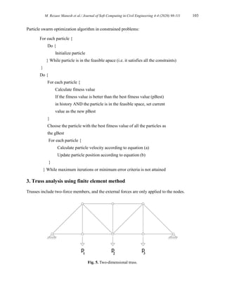
![104 M. Rezaee Manesh et al./ Journal of Soft Computing in Civil Engineering 4-4 (2020) 98-111
3.1. Local and global coordinates
Figure 6 shows a truss member and the equations for transforming two local and global
coordinates are derived:
Fig. 6. A member of truss and equations for transforming two local and global coordinates.
Local coordinate system
𝑞′
= [𝑞1
′
. 𝑞2
′
]𝑇
(3)
Global coordinate system
𝑄 = [𝑄1. 𝑄2. … . 𝑄𝑁]𝑇
(4)
The relationship between q and q' is as follows:
𝑞1
′
= 𝑞1 𝑐𝑜𝑠𝜃 + 𝑞2𝑠𝑖𝑛𝜃 (5)
𝑞2
′
= 𝑞3 𝑐𝑜𝑠𝜃 + 𝑞4𝑠𝑖𝑛𝜃 (6)
𝑞′
= 𝐿𝑞 (7)
Transformation matrix
𝐿 = [
𝑙 𝑚 0 0
0 0 𝑙 𝑚
] (8)
Calculation of m and l
𝑙 = 𝑐𝑜𝑠𝜃 =
𝑥2−𝑥1
𝑙𝑒
(9)
𝑚 = 𝑐𝑜𝑠𝜑 = 𝑠𝑖𝑛𝜃 =
𝑦2−𝑦1
𝑙𝑒
(10)](https://image.slidesharecdn.com/sccevolume4issue4pages98-111-250515104151-99302d6c/85/Dual-Target-Optimization-of-Two-Dimensional-Truss-Using-Cost-Efficiency-and-Structural-Reliability-Sufficiency-7-320.jpg)
![M. Rezaee Manesh et al./ Journal of Soft Computing in Civil Engineering 4-4 (2020) 98-111 105
𝑙𝑒 = √(𝑥2 − 𝑥1)2 + (𝑦2 − 𝑦1)2 (11)
Element stiffness matrix
Element stiffness matrix in the local coordinate system
𝑘′
=
𝐸𝑒𝐴𝑒
𝑙𝑒
[
1 − 1
−1 1
] (12)
Element stiffness matrix in the global coordinate system
The formula to calculate the strain energy in the local coordinates can be expressed as follows:
Ue =
1
2
q′T
k′
q′
(13)
𝑞′
= 𝐿𝑞 → 𝑈𝑒 =
1
2
𝑞𝑇
[𝐿𝑇
𝑘′𝐿]q (14)
The formula for calculating the strain energy in the global coordinates is as follows:
Ue =
1
2
qT
kq (15)
Element stiffness matrix in the global coordinate system
k = LT
k′
L (16)
L = [
l m 0 0
0 0 l m
] → (17)
𝑘 =
𝐸𝑒𝐴𝑒
𝑙𝑒
[
𝑙2
𝑙𝑚 − 𝑙2
− 𝑙𝑚
𝑙𝑚 𝑚2
− 𝑙𝑚 − 𝑚2
−𝑙2
− 𝑙𝑚 𝑙2
𝑙𝑚
−𝑙𝑚 − 𝑚2
𝑙𝑚 𝑚2
] (18)
The stiffness matrices of the elements combine to form the stiffness matrix of the structure.
Stress calculations
𝜎 = 𝐸𝑒𝜀 = 𝐸𝑒𝐵𝑞′
(19)
𝜎 =
𝐸𝑒
𝑙𝑒
[−1 1] {
𝑞1
′
𝑞2
′ } = 𝐸𝑒
𝑞2
′ −𝑞1
′
𝑙𝑒
(20)
𝑞′
= 𝐿𝑞 → 𝜎 =
𝐸𝑒
𝑙𝑒
[−1 1]𝐿𝑞 (21)
𝐿 = [
𝑙 𝑚 0 0
0 0 𝑙 𝑚
] → (22)
𝜎 =
𝐸𝑒
𝑙𝑒
[−𝑙 − 𝑚 𝑙 𝑚 ] (23)](https://image.slidesharecdn.com/sccevolume4issue4pages98-111-250515104151-99302d6c/85/Dual-Target-Optimization-of-Two-Dimensional-Truss-Using-Cost-Efficiency-and-Structural-Reliability-Sufficiency-8-320.jpg)
![106 M. Rezaee Manesh et al./ Journal of Soft Computing in Civil Engineering 4-4 (2020) 98-111
4. Numerical example of single-objective truss optimization
4.1. Particle swarm optimization
In the example of the optimization of a conventional truss [17], which was analyzed by various
methods so far, it is optimized by particle swarm optimization (PSO) algorithm method and the
final result is compared with other methods. For this purpose, the total number of particles is
considered to be 60, and the constant values of w, c1, and c2 are selected as 0.5, 1.5, and 1.5,
respectively. The algorithm code is written in the MATLAB software and the structure is
analyzed using the stiffness matrix (finite element) method.
Fig. 7. 10-bar truss from [17].
Table 1
Parameters related to Fig. 7.
Parameter Value Unit
E 104 𝑘𝑠𝑖
𝜌 0.1 𝑙𝑏𝑚 𝑖𝑛3
⁄
𝜎𝑎𝑙𝑙𝑜𝑤 25000 psi
𝑑𝑚𝑎𝑥 2 in
L 360 in
P 100 kip
Consider the 10-bar truss in Figure 1 which was studied to compare and verify the algorithm.
The purpose of the problem is to minimize the weight of the structure f(x):
𝑓(𝑥) = ∑ (𝜌 𝐴𝑖 𝐿𝑖 )
10
𝑛=1 (24)
x is the solution to the problem, Ai is the cross-sectional area of bar i, Li is the length of bar i, and
ρ is the weight density:
𝜌 = 0.10 𝐼𝑏
𝑖𝑛3
⁄ (2770
𝑘𝑔
𝑚3
⁄ ) (25)](https://image.slidesharecdn.com/sccevolume4issue4pages98-111-250515104151-99302d6c/85/Dual-Target-Optimization-of-Two-Dimensional-Truss-Using-Cost-Efficiency-and-Structural-Reliability-Sufficiency-9-320.jpg)
![M. Rezaee Manesh et al./ Journal of Soft Computing in Civil Engineering 4-4 (2020) 98-111 107
The elastic modulus 𝐸 = 1 × 10⁴
𝑘𝑠𝑖 (6.89 × 10⁴
𝑀𝑝𝑎) and downward external force
100 𝑘𝑖𝑝𝑠 (445.374 𝐾𝑁) are applied to nodes 2 and 4.
The truss constraints are:
𝜎𝑖 ≤ 𝜎𝑎𝑙𝑙 𝑖 = 1: 10 (26)
𝑢𝑖 ≤ 𝑢𝑎 (27)
where σi is the stress in bar i and σall is the maximum allowable stress for all bars, ui is the
displacement of each node (horizontal and vertical), and ua is the maximum allowable
displacement for all nodes.
𝑢𝑎 = 2 𝑖𝑛 (50.8 𝑚𝑚) (28)
𝜎𝑎𝑙𝑙 = ±25 𝐾𝑠𝑖 (172.25 𝑀𝑝𝑎) (29)
This problem is optimized using the PSO algorithm, and the results are summarized in Table 2;
To compare with the results of Table 3, the problem is optimized twice (the cross-sectional area
of the bars is considered in two different ranges):
Table 2
Results from the optimization of 10-bar truss size using PSO algorithm method, first run.
𝟎. 𝟏 ≤ 𝑨𝒊 (𝒊𝒏𝟐) ≤ 𝟑𝟑. 𝟓, Iteration: 50
A10
A9
A8
A7
A6
A5
A4
A3
A2
A1
Weight (lb)
Method
0.1
21.03
20.85
7.28
0.1
0.1
16.80
26.16
0.1
31.18
5187.4
PSO
(obtained Results)
Table 3
Results from the optimization of 10-bar truss size using PSO algorithm method, second run.
𝟏. 𝟔𝟐 ≤ 𝑨𝒊 (𝒊𝒏𝟐
) ≤ 𝟑𝟑. 𝟓, Iteration: 50
A10
A9
A8
A7
A6
A5
A4
A3
A2
A1
Weight (lb)
Method
1.62
21.52
22.56
8.37
1.62
1.62
17.08
25.89
1.62
32.2
5636.2
PSO
(obtained Results)
Table 4
Results from the optimization of 10-bar truss size from [17].
A10
(𝒊𝒏𝟐
)
A9
(𝒊𝒏𝟐
)
A8
(𝒊𝒏𝟐
)
A7
(𝒊𝒏𝟐
)
A6
(𝒊𝒏𝟐
)
A5
(𝒊𝒏𝟐
)
A4
(𝒊𝒏𝟐
)
A3
(𝒊𝒏𝟐
)
A2
(𝒊𝒏𝟐
)
A1
(𝒊𝒏𝟐
)
Weight
(lb)
Method
1.14
20.74
20.32
15.40
0.10
0.10
19.39
25.11
0.10
25.70
5472.00
OPTDYN
2.51
20.98
19.73
16.67
1.75
0.10
15.83
24.87
1.89
25.20
5563.00
CONMIN
2.62
19.90
19.90
14.20
1.80
1.62
15.50
22.00
1.62
33.50
5620.08
GENETIC
2.62
19.90
19.90
14.20
1.62
1.62
15.50
22.00
1.62
33.50
5613.84
Rajeev
4.42
18.76
19.17
19.34
3.43
0.10
12.77
26.42
3.07
25.84
5719.00
M-3
4.38
18.77
19.18
19.37
3.77
0.10
12.75
26.45
2.88
25.83
5725.00
M-5
5.26
19.27
19.26
17.46
4.17
0.10
14.45
24.78
4.17
24.78
5727.00
GRP-UI
3.26
13.97
20.90
21.71
3.71
0.10
11.66
31.62
2.37
30.69
5932.00
SUMT
13.51
18.40
18.42
18.91
10.98
0.10
14.95
22.08
10.98
21.57
6249.00
LINRM](https://image.slidesharecdn.com/sccevolume4issue4pages98-111-250515104151-99302d6c/85/Dual-Target-Optimization-of-Two-Dimensional-Truss-Using-Cost-Efficiency-and-Structural-Reliability-Sufficiency-10-320.jpg)
![108 M. Rezaee Manesh et al./ Journal of Soft Computing in Civil Engineering 4-4 (2020) 98-111
The comparison of the obtained results with [17] confirms the PSO algorithm used in this
research for the truss optimization.
4.2. Structural reliability analysis
In this section, the reliability level of the truss system is determined to evaluate the difference
between the available optimization approaches. The reliability analysis process is established
based on the provided framework by Ghasemi and Nowak [18,19]. To do so, two types of the
limit state functions based on the ultimate limit state function (ULSF).
ULSF: 𝑔𝑢 = 𝜎𝑦 −
𝑃
𝐴
(30)
where 𝑔𝑢 and 𝑔𝑠 stand as the ultimate and service limit state functions, respectively. P is the
element’s load; A represents the optimum value of the element’s cross-section. Tables 5 shows
the reliability indices of each truss element, corresponding to the considered optimization
approaches. It is worth mentioning that the reliability index is simply taken from FORM methods
as shown in the following equation [20].
𝛽𝑒 =
𝑅𝑛.𝜆𝑅−𝑄𝑛𝜆𝑄
√𝜎𝑅
2+𝜎𝑄
2
(31)
where 𝑅𝑛 and 𝑄𝑛 are the nominal value of the structural resistance (nominal value of 𝜎𝑦for
USLF and nominal value of 𝛼𝐿for SLSF) and nominal value of loads. 𝜆𝑅and 𝜆𝑄denote the bias
factor (mean over nominal value) of resistance and load. Also, 𝜎𝑅and 𝜎𝑄are the standard
deviation of the resistance and load. The statistical parameter of both resistance and load can be
taken from Ghasemi and Lee [21].
Table 5
Reliability indices of each element corresponding to the given optimization approaches concerning ULSF.
Method Weight (lb) A1 A2 A3 A4 A5 A6 A7 A8 A9 A10
OPTDYN 5472.00 8.48 -9.10 5.12 8.62 -9.6 -9.10 2.68 10 8.15 -2.44
CONMIN 5563.00 8.45 -3.18 5.08 9.57 -8.39 -3.65 3.18 10 9.55 -3.56
GENETIC 5620.08 8.85 3.34 4.45 8.14 -3.42 3.96 2.15 10 7.94 4.13
Rajeev 5613.84 8.85 3.46 4.45 8.12 -3.47 3.46 2.15 10 7.92 4.24
M-3 5719.00 8.49 -0.47 5.37 9.68 -7.30 0.31 4.06 10 9.69 -0.34
M-5 5725.00 8.49 -0.92 5.37 9.68 -7.30 0.98 4.07 10 9.69 -0.41
GRP-UI 5727.00 8.42 1.53 5.06 9.77 -6.71 1.53 3.46 10 9.75 0.74
SUMT 5932.00 8.75 -2.08 6.14 9.58 -7.77 1.04 4.69 10 9.50 -2.27
LINRM 6249.00 8.17 6.44 4.47 9.91 -2.13 6.44 3.93 10 9.89 5.89
PSO 5636.20 8.80 4.64 5.27 8.19 -3.85 4.64 -1.53 10 7.95 2.59](https://image.slidesharecdn.com/sccevolume4issue4pages98-111-250515104151-99302d6c/85/Dual-Target-Optimization-of-Two-Dimensional-Truss-Using-Cost-Efficiency-and-Structural-Reliability-Sufficiency-11-320.jpg)
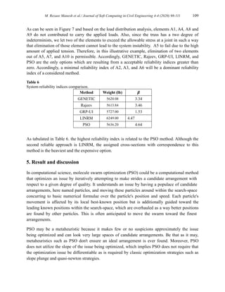
![110 M. Rezaee Manesh et al./ Journal of Soft Computing in Civil Engineering 4-4 (2020) 98-111
PSO has to been connected to multi-objective issues, in which the objective work comparison
takes Pareto dominance into consideration when moving the PSO particles and non-dominated
arrangements are put away to inexact the Pareto front. Multi-swarm optimization could be a
variation of particle swarm optimization (PSO) based on the utilize of numerous sub-swarms
rather than one (standard) swarm. The common approach in multi-swarm optimization is that
each sub-swarm centers on a particular locale whereas a particular enhancement strategy chooses
where and when to dispatch the sub-swarms. The multi-swarm system is particularly fitted for
the optimization of multi-modal issues, where numerous (local) optima exist.
6. Conclusions
In this paper, a two-dimensional truss was analyzed with the finite element method and
optimized using the PSO algorithm and then, the optimization results were compared with those
of [17]. The analysis of comparisons suggests that the PSO algorithm leads to better results in
terms of the higher convergence rate. Comparing the results with this reference shows confirms
the PSO algorithm in this paper for truss optimization. It seems that the PSO algorithm (bird
algorithm) is a good choice for the optimization of trusses and has an acceptably high rate of
convergence. This method is dependent on the values of ω, c1, and c2, and the values suggested in
this paper can be used as the initial data. The number of particles (birds) is also important in this
algorithm, but it is less important than the above factors and can be considered from 40 to 70.
By the way, this problem opens two main question in structural optimizations. The first question
is to how establish a framework to determine the reliability index of a system associated with the
different degree of indeterminacies? And the second question is how to make a decision of
optimization approach selection with consideration of both cost and reliability? The
methodologies of addressing the responses to the above-mentioned questions are expected to be
conducted in future studies. This, this paper attempts to shed more light to address the concern of
the system reliability with various possible redundancy and target reliability selection associated
with cost and reliability.
References
[1] Cui Z, Gao X. Theory and applications of swarm intelligence. Neural Comput Appl 2012;21:205–
6. doi:10.1007/s00521-011-0523-8.
[2] Dorigo M, Blum C. Ant colony optimization theory: A survey. Theor Comput Sci 2005;344:243–
78. doi:10.1016/j.tcs.2005.05.020.
[3] Antoniou P, Pitsillides A, Blackwell T, Engelbrecht A. Employing the flocking behavior of birds
for controlling congestion in autonomous decentralized networks. 2009 IEEE Congr Evol Comput,
IEEE; 2009, p. 1753–61. doi:10.1109/CEC.2009.4983153.
[4] Antoniou P, Pitsillides A, Blackwell T, Engelbrecht A, Michael L. Congestion control in wireless
sensor networks based on bird flocking behavior. Comput Networks 2013;57:1167–91.
doi:10.1016/j.comnet.2012.12.008.](https://image.slidesharecdn.com/sccevolume4issue4pages98-111-250515104151-99302d6c/85/Dual-Target-Optimization-of-Two-Dimensional-Truss-Using-Cost-Efficiency-and-Structural-Reliability-Sufficiency-13-320.jpg)
![M. Rezaee Manesh et al./ Journal of Soft Computing in Civil Engineering 4-4 (2020) 98-111 111
[5] Karaboga D, Basturk B. On the performance of artificial bee colony (ABC) algorithm. Appl Soft
Comput 2008;8:687–97. doi:10.1016/j.asoc.2007.05.007.
[6] Karaboga D, Basturk B. A powerful and efficient algorithm for numerical function optimization:
artificial bee colony (ABC) algorithm. J Glob Optim 2007;39:459–71. doi:10.1007/s10898-007-
9149-x.
[7] Li XL, Qian JX. Studies on artificial fish swarm optimization algorithm based on decomposition
and coordination techniques. J Circuits Syst 2003;1:1–6.
[8] Neshat M. FAIPSO: fuzzy adaptive informed particle swarm optimization. Neural Comput Appl
2013;23:95–116. doi:10.1007/s00521-012-1256-z.
[9] Chen D, Zhao C, Zhang H. An improved cooperative particle swarm optimization and its
application. Neural Comput Appl 2011;20:171–82. doi:10.1007/s00521-010-0503-4.
[10] Kennedy J, Eberhart R. Particle swarm optimization. Proc IEEE Int Conf Neural Netw IV, 1942–
1948, vol. 4, IEEE; 1995, p. 1942–8. doi:10.1109/ICNN.1995.488968.
[11] Eberhart R, Kennedy J. A new optimizer using particle swarm theory. MHS’95 Proc Sixth Int
Symp Micro Mach Hum Sci, IEEE; n.d., p. 39–43. doi:10.1109/MHS.1995.494215.
[12] Hajihassani M, Jahed Armaghani D, Kalatehjari R. Applications of Particle Swarm Optimization in
Geotechnical Engineering: A Comprehensive Review. Geotech Geol Eng 2018;36:705–22.
doi:10.1007/s10706-017-0356-z.
[13] Zhu H, Wang Y, Wang K, Chen Y. Particle Swarm Optimization (PSO) for the constrained
portfolio optimization problem. Expert Syst Appl 2011;38:10161–9.
[14] Shi Y, Eberhart R. A modified particle swarm optimizer. 1998 IEEE Int Conf Evol Comput
proceedings IEEE world Congr Comput Intell (Cat No 98TH8360), IEEE; 1998, p. 69–73.
[15] Poitras G, Lefrançois G, Cormier G. Optimization of steel floor systems using particle swarm
optimization. J Constr Steel Res 2011;67:1225–31.
[16] Kalatehjari R. An improvised three-dimensional slope stability analysis based on limit equilibrium
method by using particle swarm optimization 2013.
[17] Rajeev S, Krishnamoorthy CS. Discrete optimization of structures using genetic algorithms. J
Struct Eng 1992;118:1233–50.
[18] Ghasemi SH, Nowak AS. Reliability index for non-normal distributions of limit state functions.
Struct Eng Mech 2017;62:365–72. doi:10.12989/sem.2017.62.3.365.
[19] Ghasemi SH, Nowak AS. Target reliability for bridges with consideration of ultimate limit state.
Eng Struct 2017;152:226–37. doi:10.1016/j.engstruct.2017.09.012.
[20] Reliability analysis of circular tunnel with consideration of the strength limit state n.d.
doi:https://doi.org/10.12989/gae.2018.15.3.879.
[21] Ghasemi SH, Lee JY. Reliability-based indicator for post-earthquake traffic flow capacity of a
highway bridge. Struct Saf 2021;89:102039. doi:10.1016/j.strusafe.2020.102039.](https://image.slidesharecdn.com/sccevolume4issue4pages98-111-250515104151-99302d6c/85/Dual-Target-Optimization-of-Two-Dimensional-Truss-Using-Cost-Efficiency-and-Structural-Reliability-Sufficiency-14-320.jpg)
The main contribution of this study is to open a discussion regarding the structural optimization associated with the cost efficiency and structural reliability sufficiency consideration. To do so, several various optimization approaches are investigated to deliberate both cost and reliability concerns. Particularly, particle swarm optimization is highlighted as a reliable optimization approach. Accordingly, an illustrative example is rendered to compare the feasibility of the considered optimization approaches. The feasibility of the investigated approaches is evaluated using the cost and reliability analysis. For the considered example, it was observed that the PSO optimization algorithm has multiple advantages such as easy realization, fast convergence, and promising performance in nonlinear performance optimization. The PSO optimization algorithm can be successfully applied in various fields of civil engineering. This popularity is due to the understandable performance of the PSO as well as its simplicity. In this paper, first, the literature on the subject has been described by two-dimensional truss analysis using the finite element method and optimized using the PSO particle swarm algorithm. A comparison of the results with this reference indicates the accuracy of this particle swarm algorithm in truss optimization. Indeed, this study ignites two main insights in structural optimizations assessment. The first illustration is related to how to establish a framework for structural system reliability analysis associated with the different degrees of indeterminacies. And the second illustration is related to making a decision problem concerning the structural optimization while both cost and reliability metric are two main parameters for the construction point of the view.