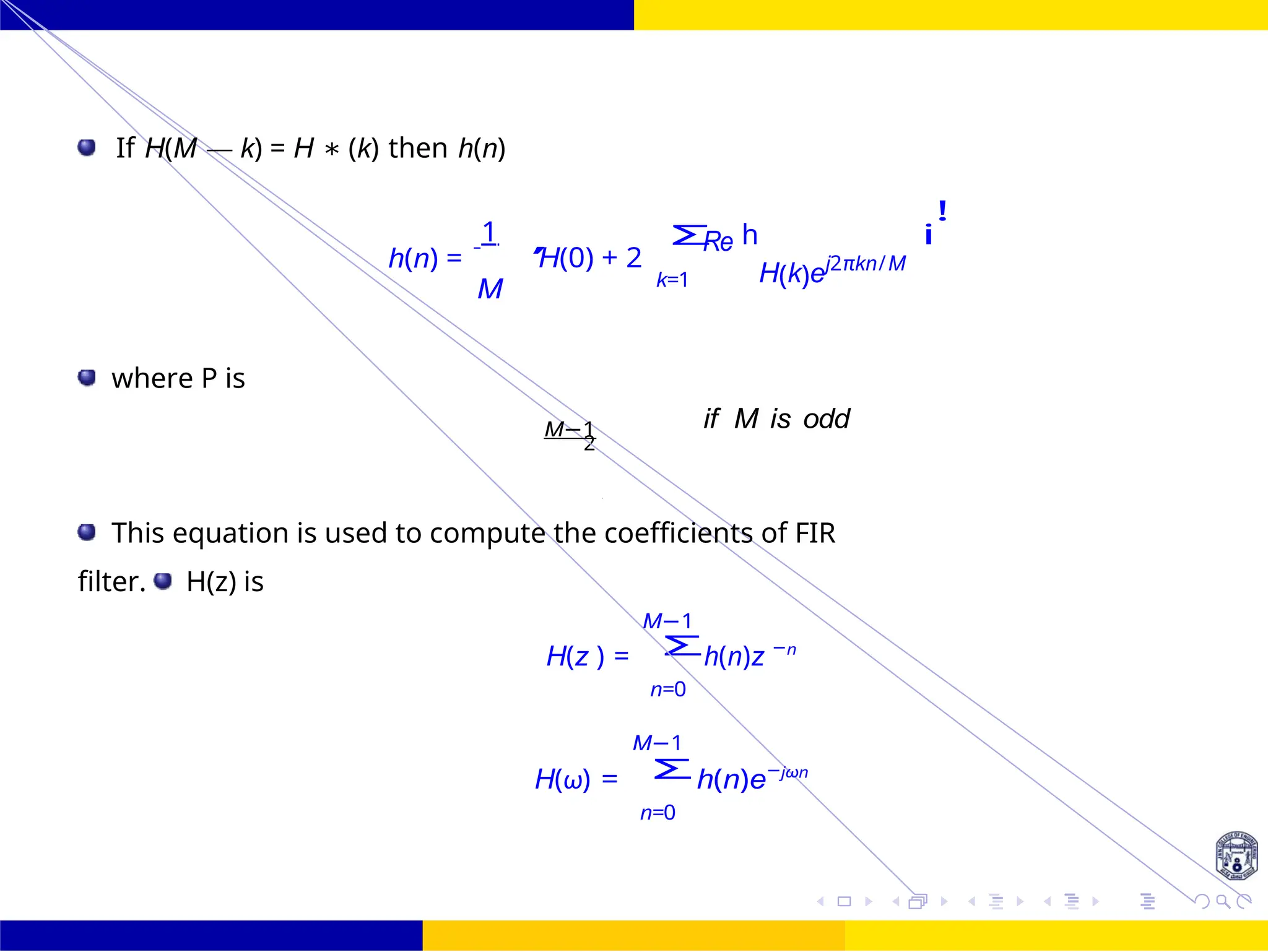
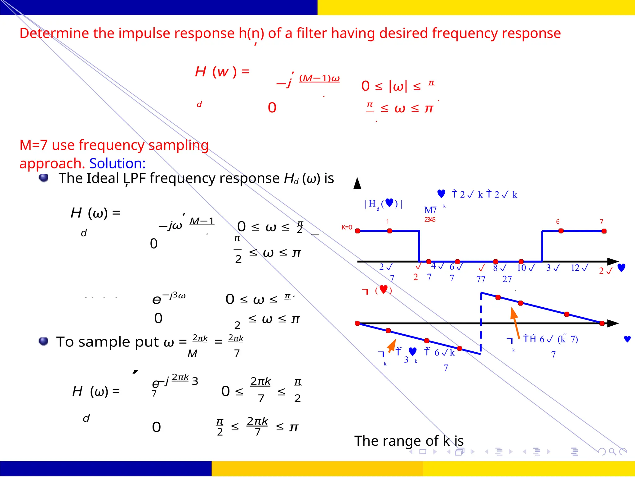
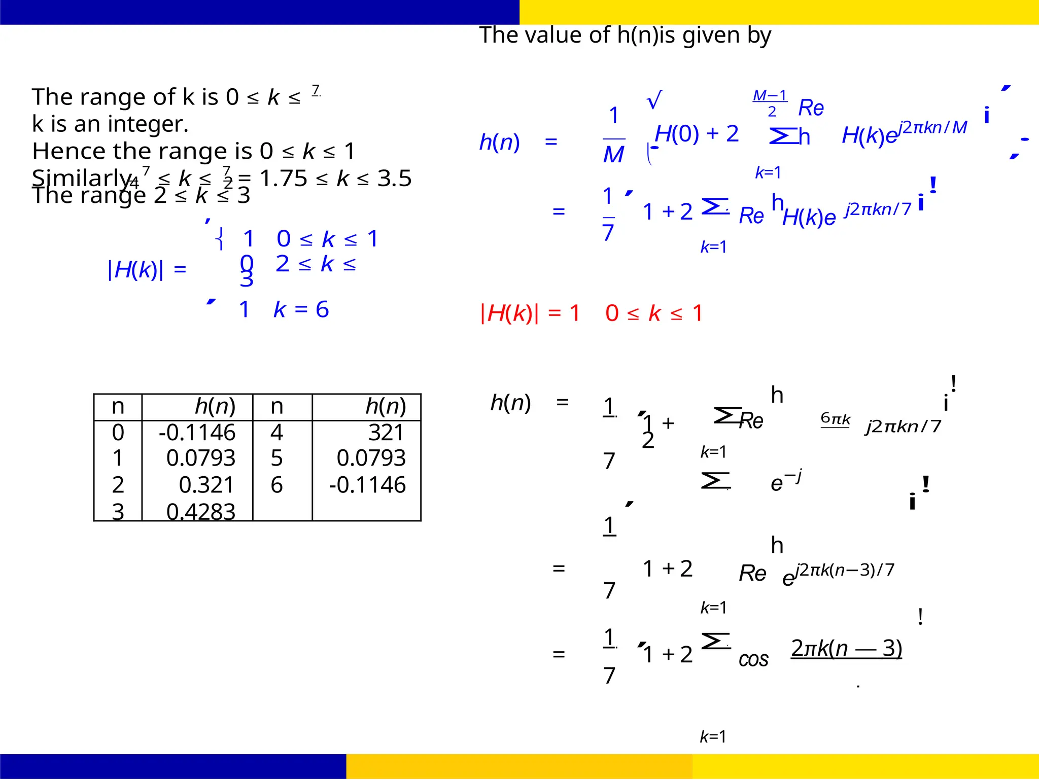
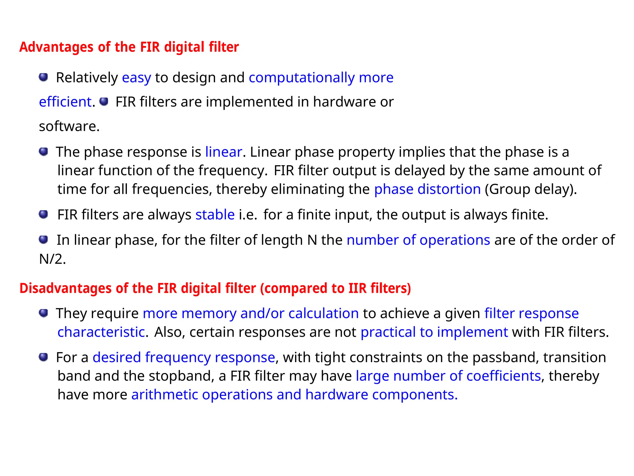
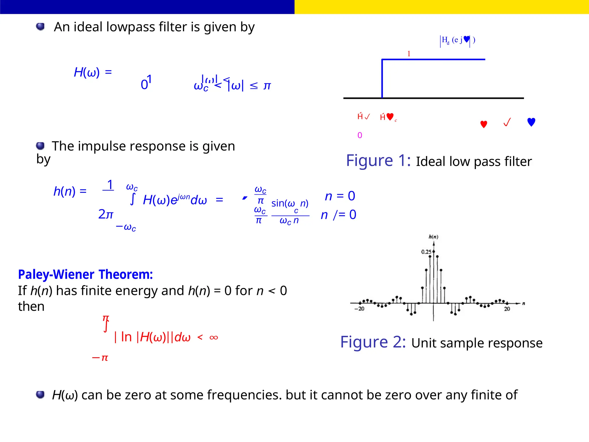
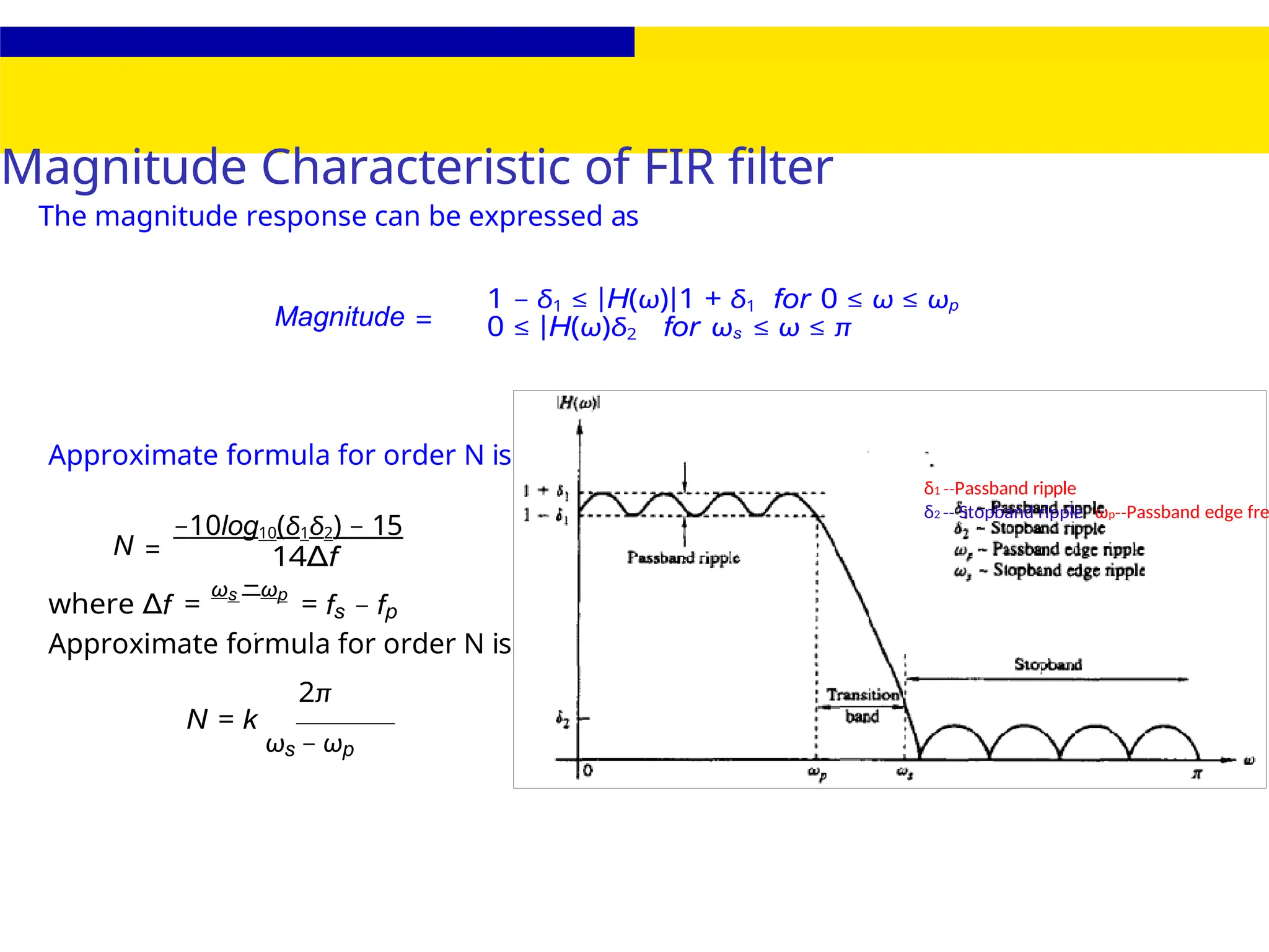
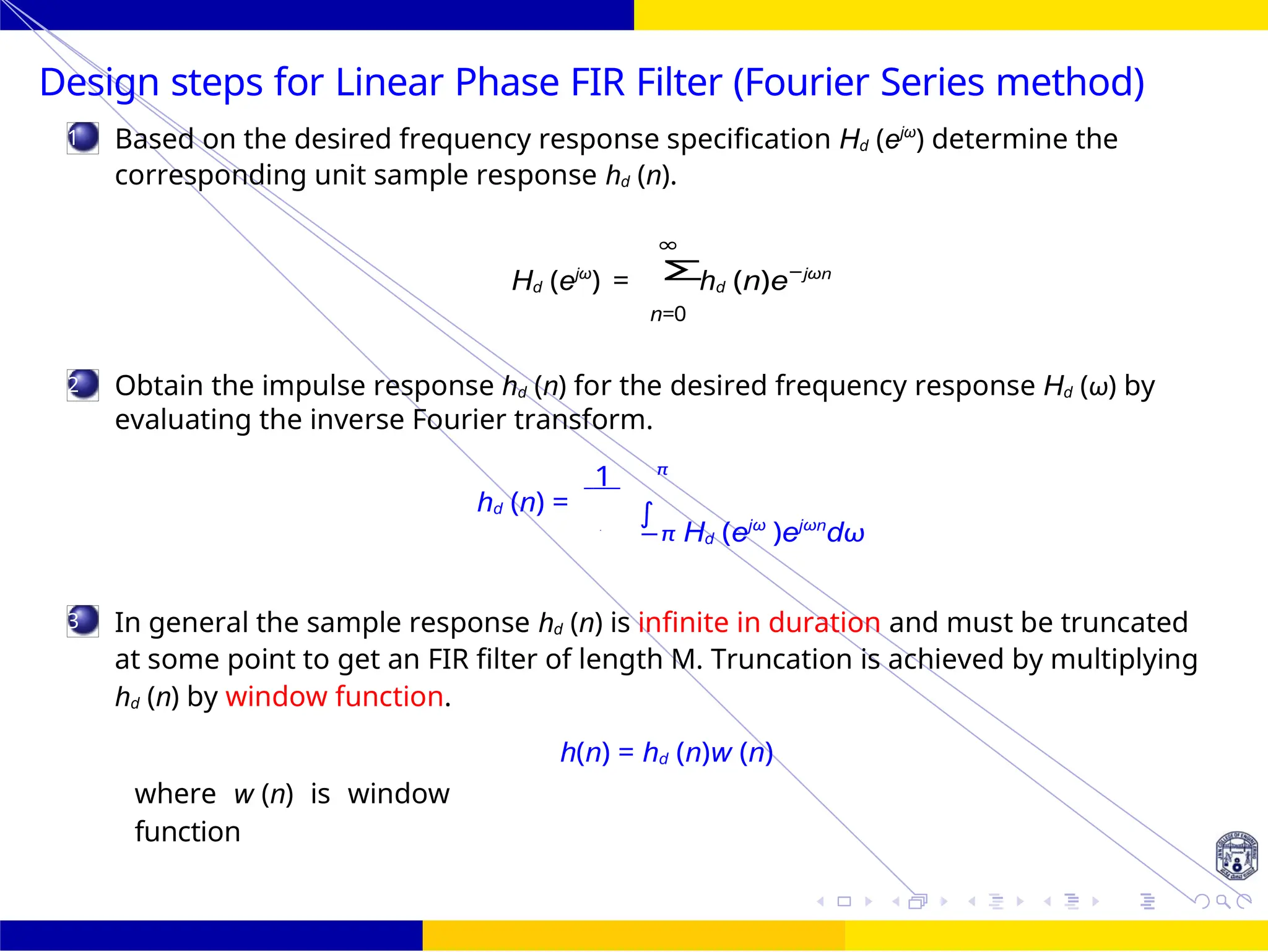
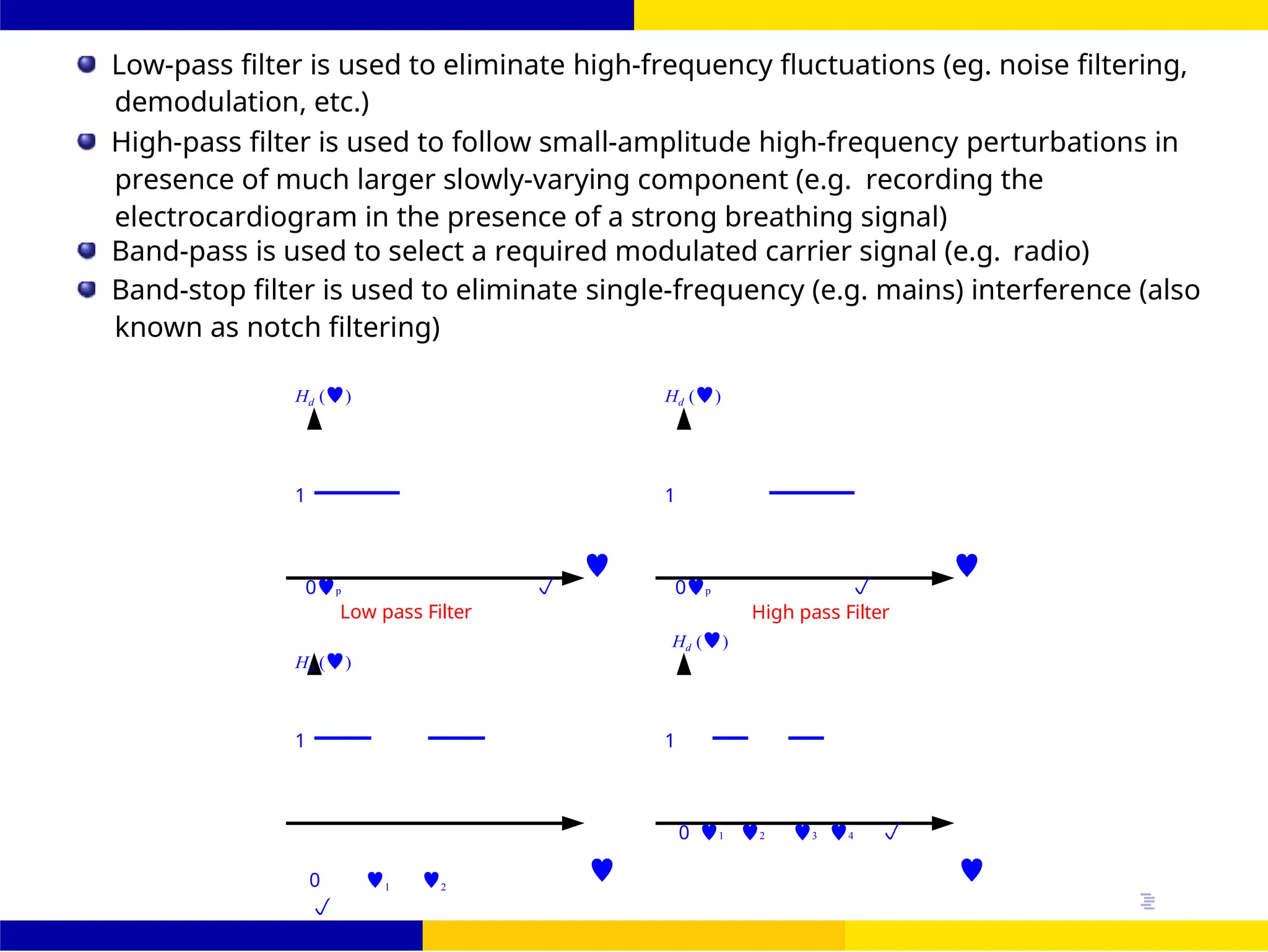
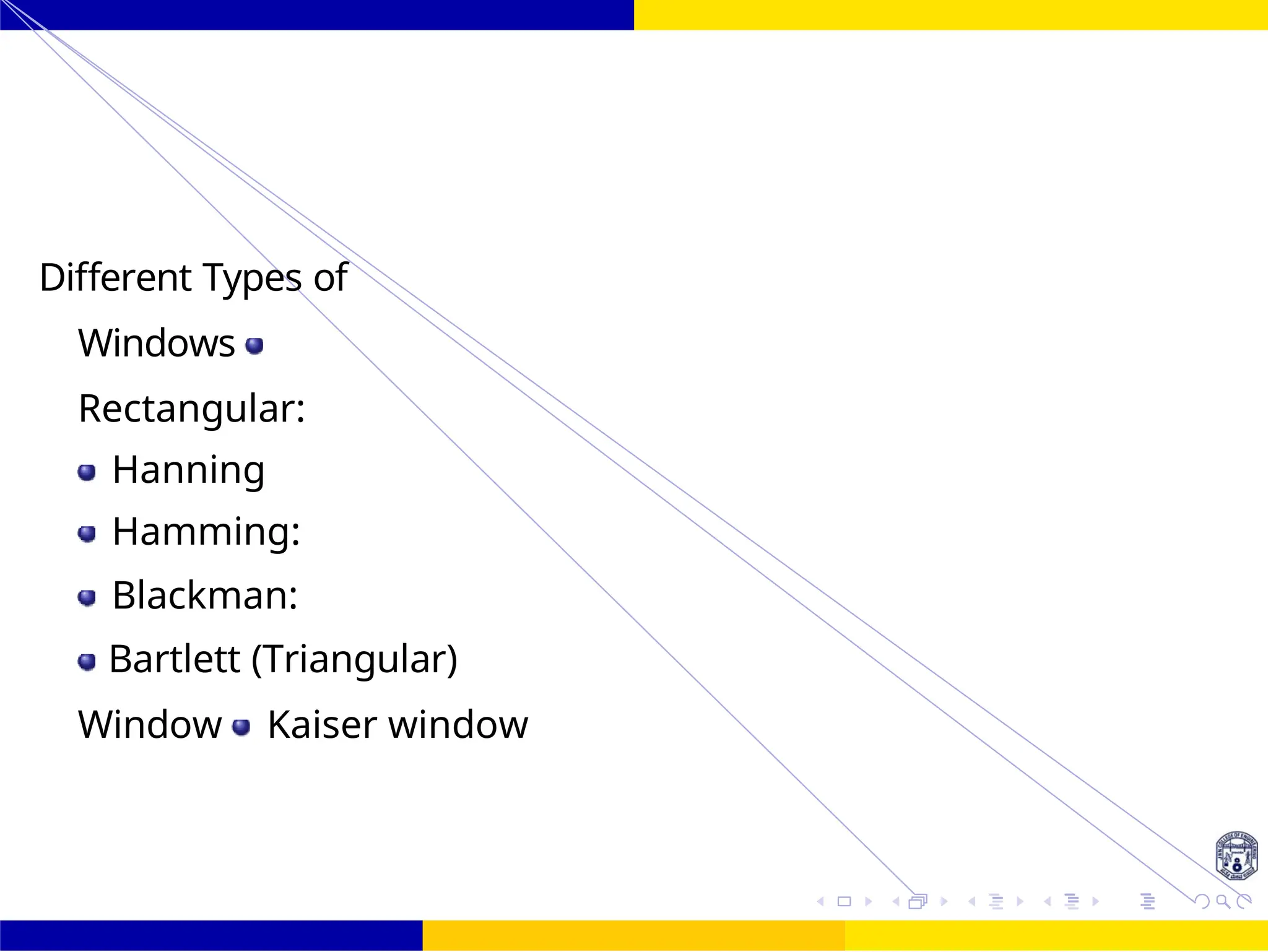
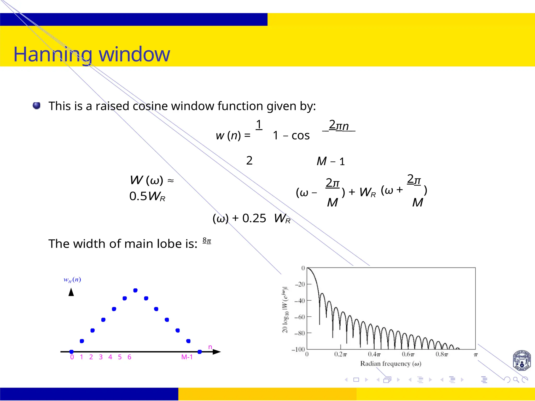
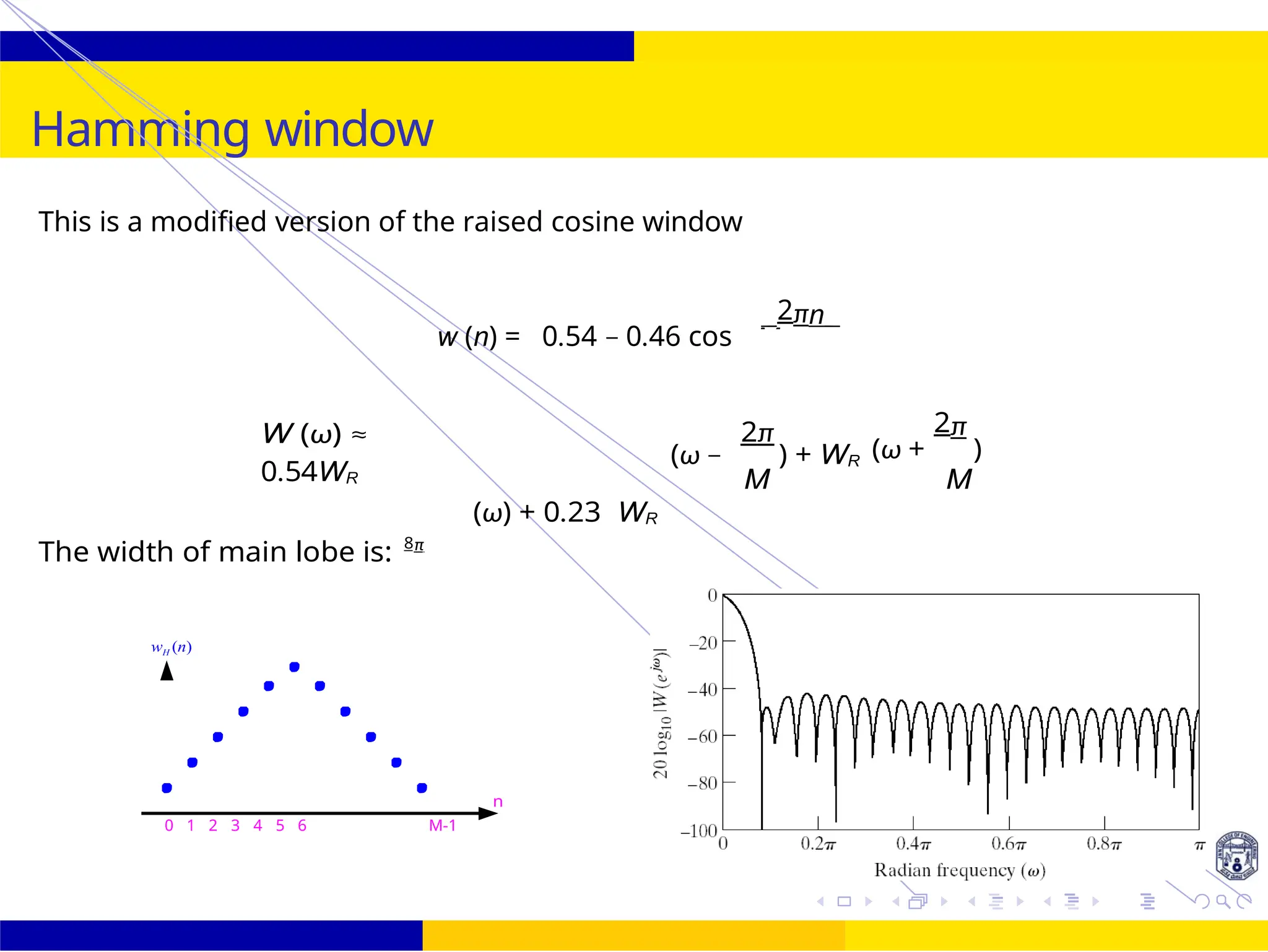
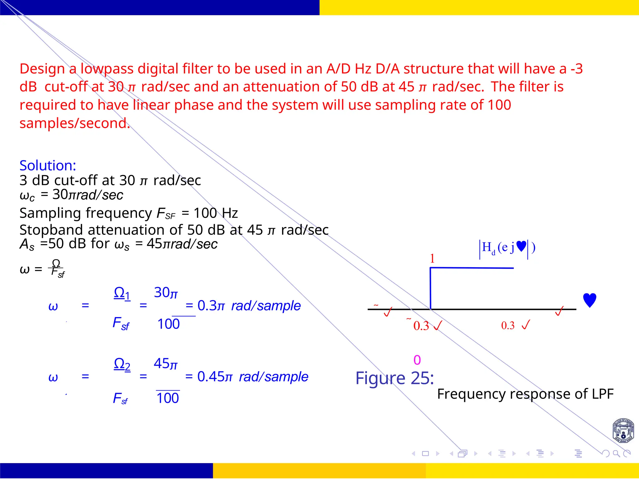
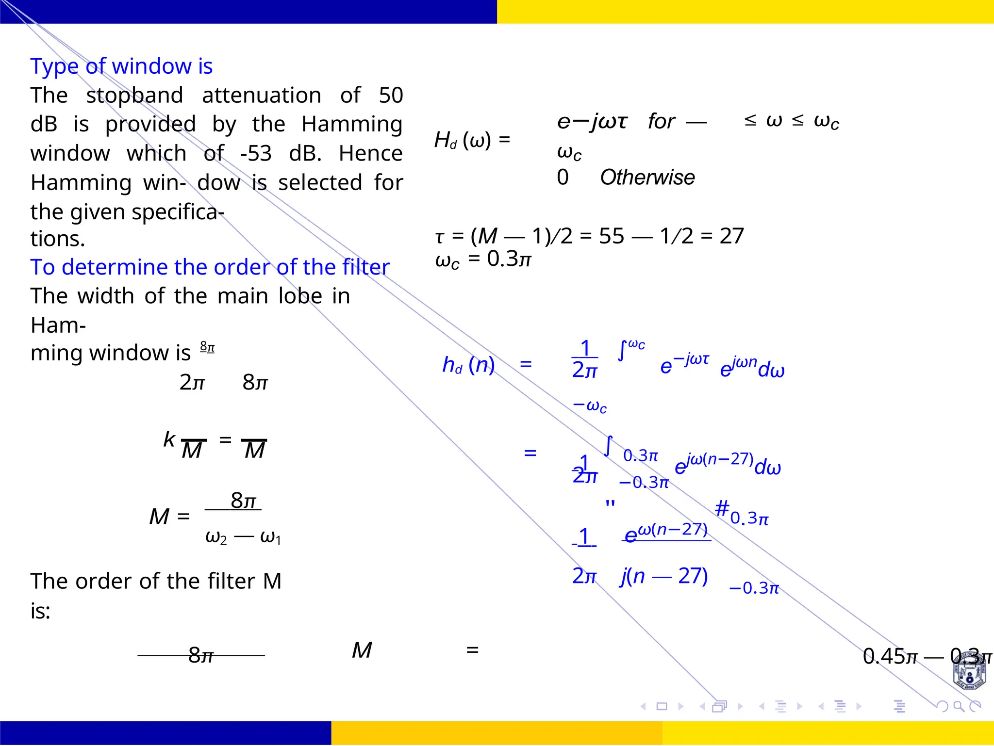
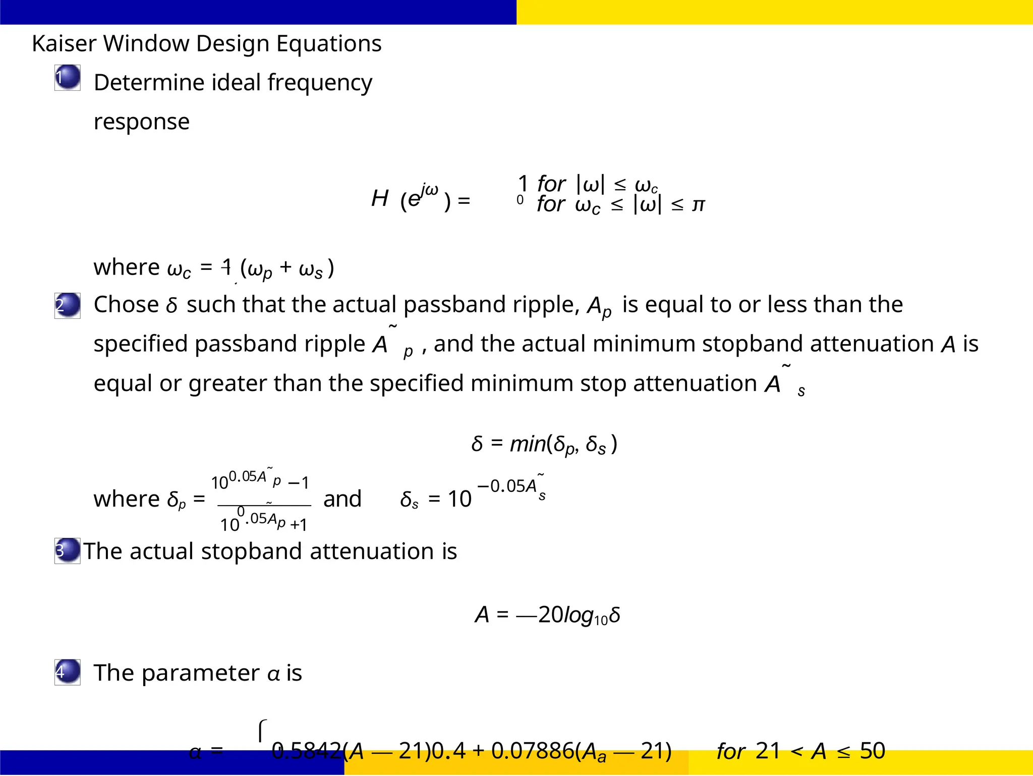
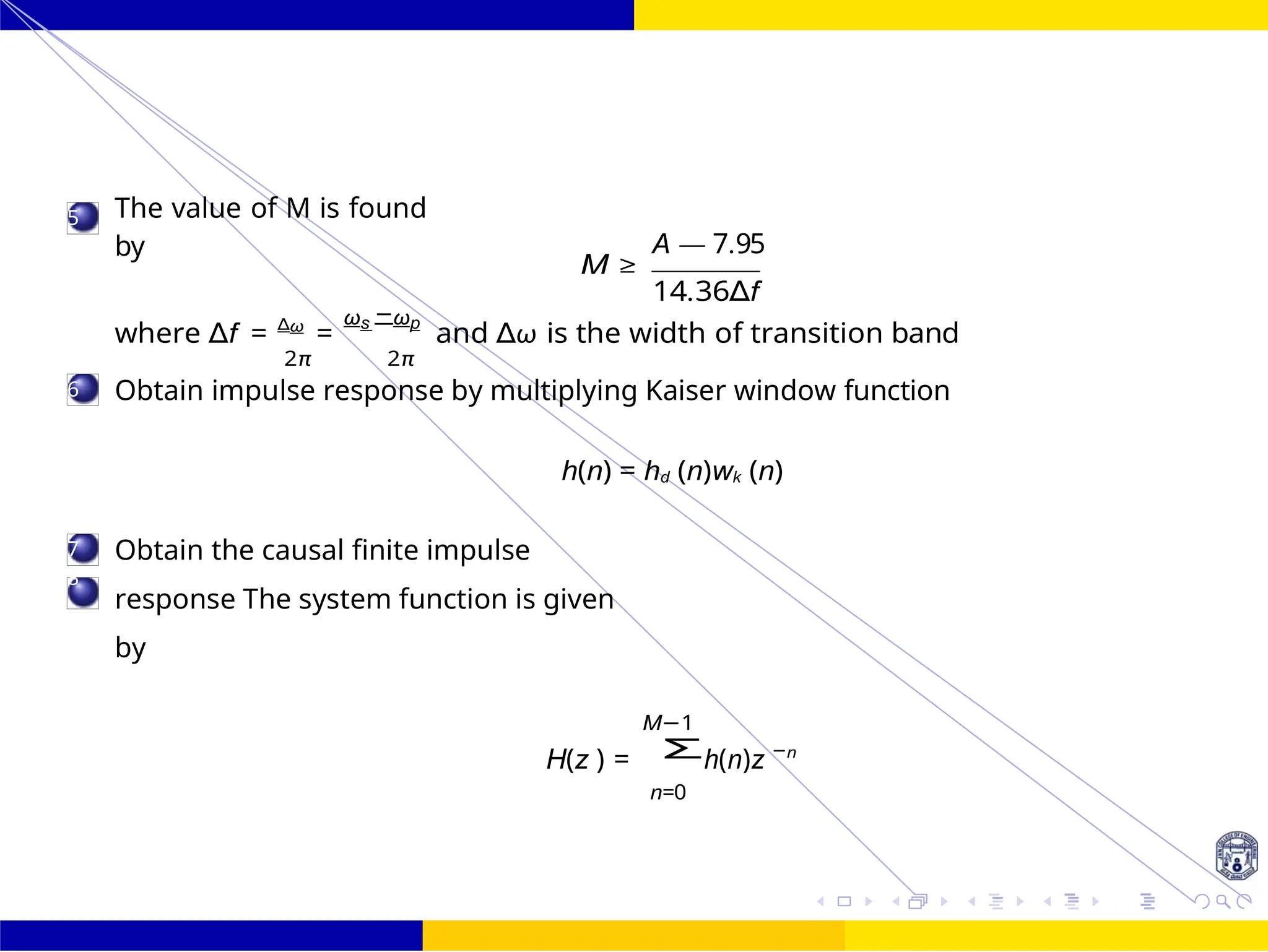
The document discusses FIR filter design, covering the advantages such as linear phase response, stability, and computational efficiency, as well as the disadvantages compared to IIR filters. It details the mathematical foundations and techniques for designing FIR filters, including methods using different window functions and frequency sampling techniques. Additionally, it addresses properties such as symmetry, phase distortion avoidance, and magnitude response characteristics relevant to various filter types.
![An LTI system is causal iff
Input/output relationship: y [n] depends only on current and past input signal
values. Impulse response: h[n] = 0 for n < 0
System function: number of finite zeros ≤ number of finite poles.](https://image.slidesharecdn.com/dspmodule4ppt-241209183808-f5b6e07b/75/dsp-module-4-pptpptrpppptxppppppppp-docx-5-2048.jpg)
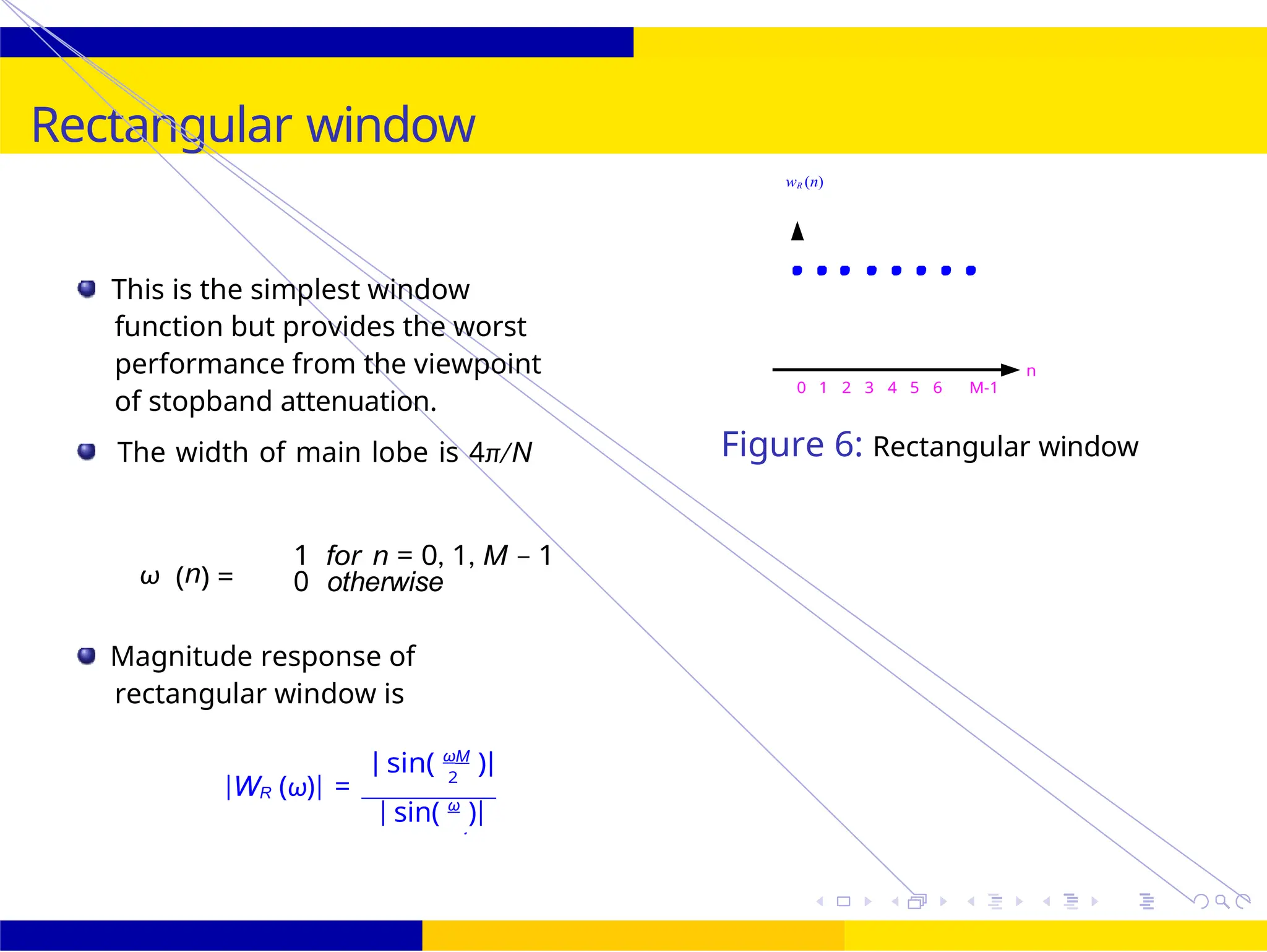
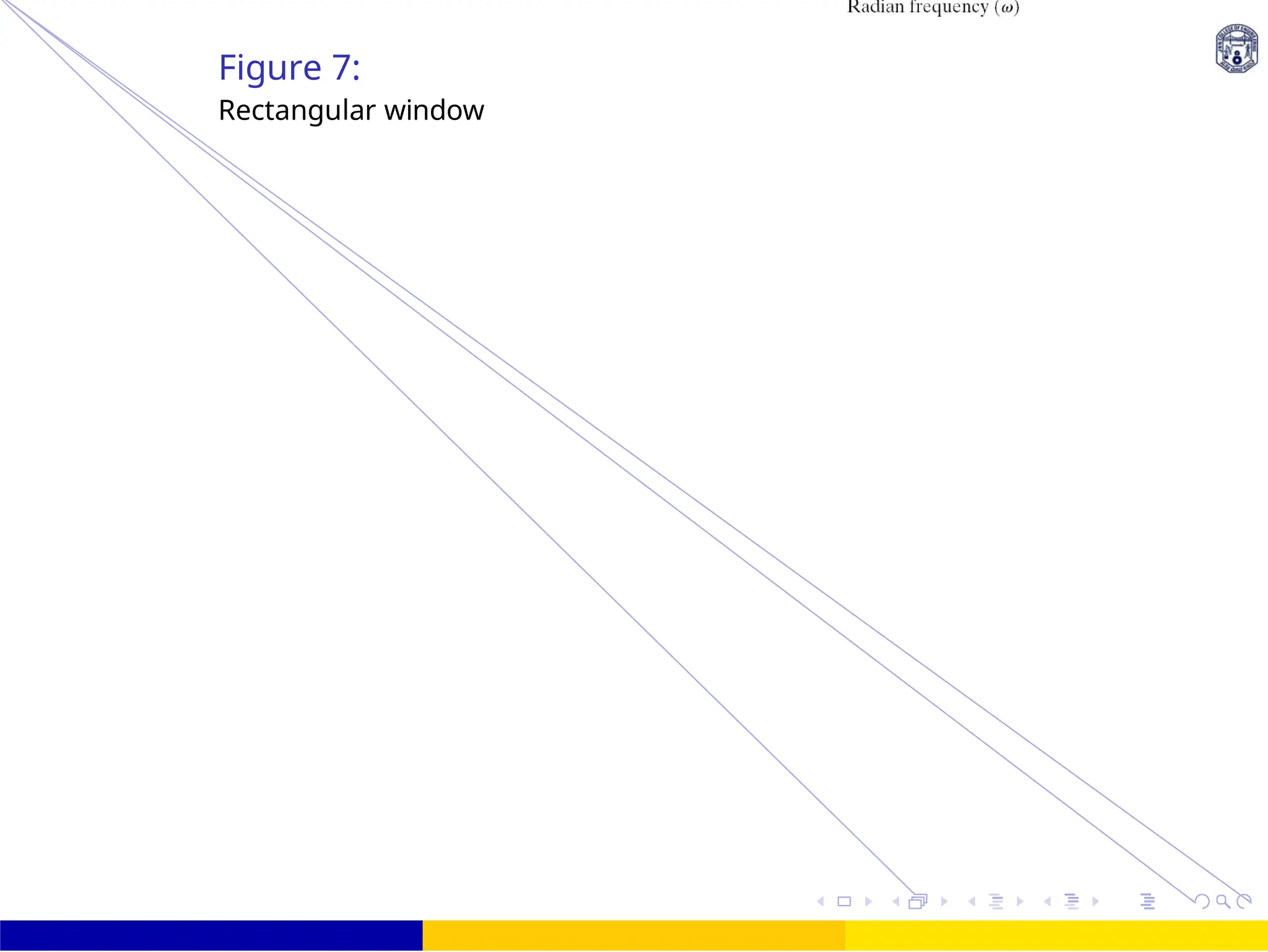
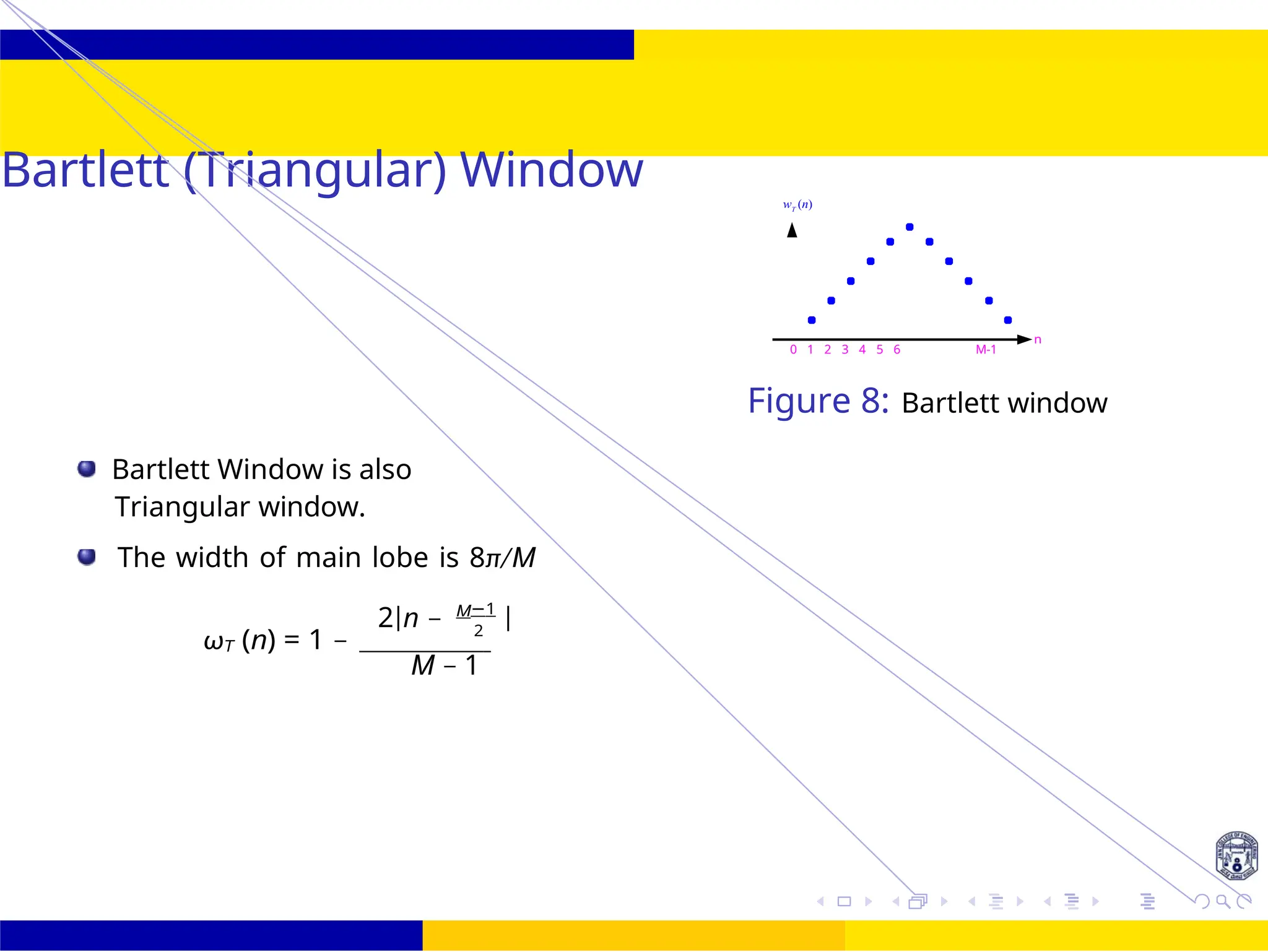
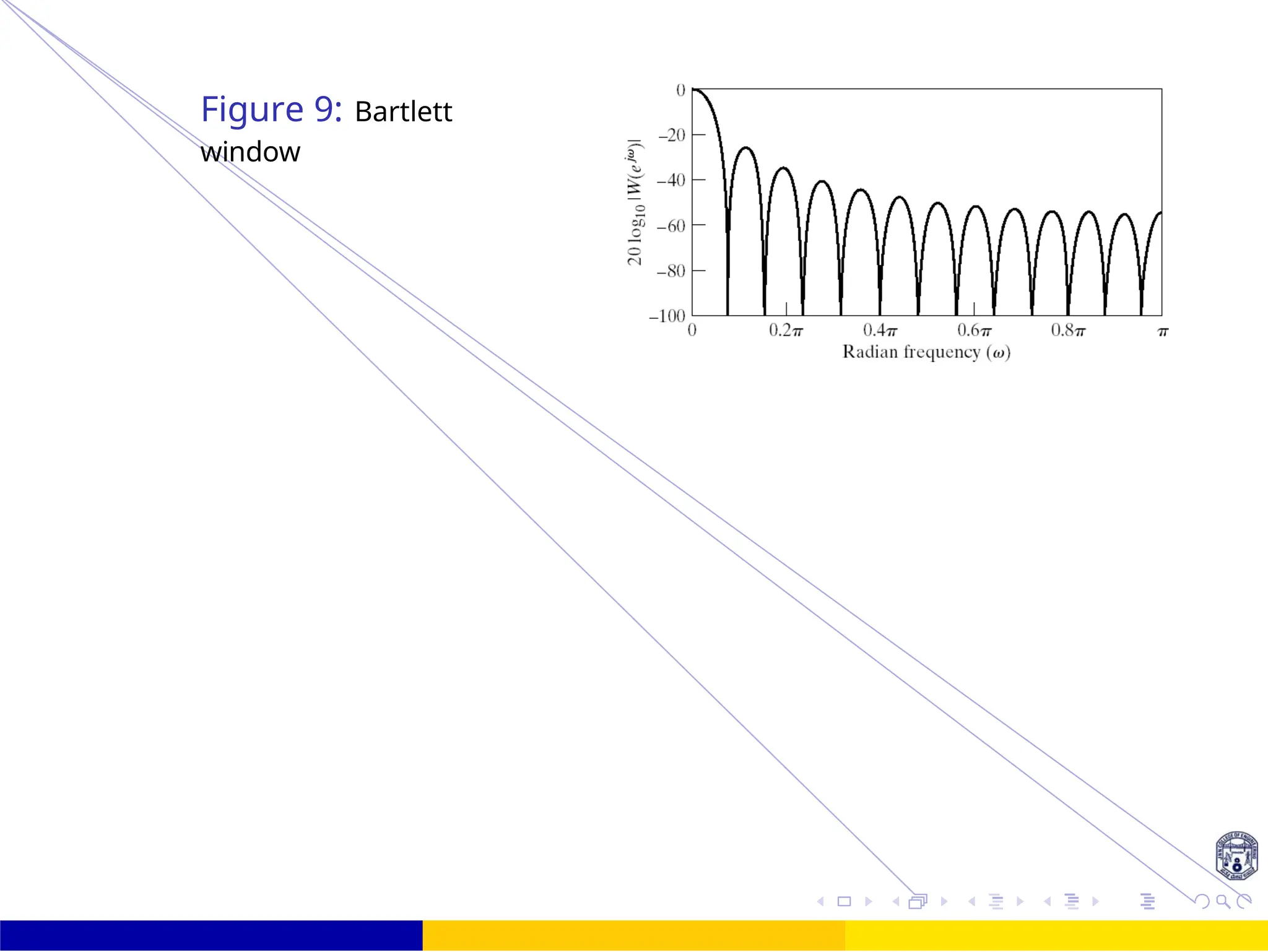
![FIR Filter Design
frequencies, since the integral then becomes infinite.
H(ω) cannot be exactly zero over any band of frequencies. (Except in the trivial case where
h[n]
= 0.) Furthermore, |H(ω)| cannot be flat (constant) over any finite band.](https://image.slidesharecdn.com/dspmodule4ppt-241209183808-f5b6e07b/75/dsp-module-4-pptpptrpppptxppppppppp-docx-7-2048.jpg)


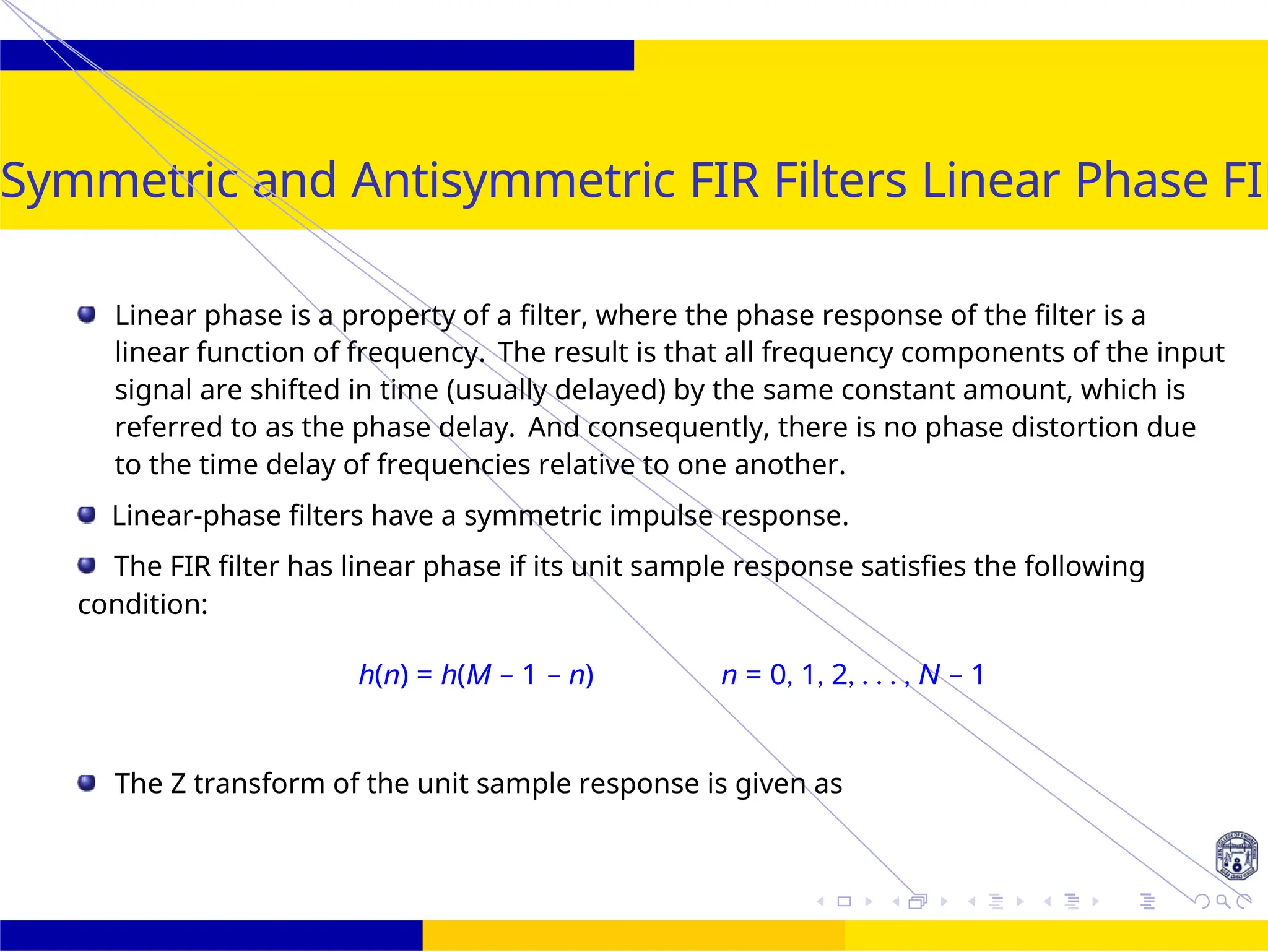
![FIR Filter Design Symmetric and Antisymmetric FIR
Filters
UNIT - 7: FIR Filter October 25, 17 /
0 1 2 3 4 5 6 7 8n
Center of Symmetry
0 1 2 3 4 5 6 7 8n
0 1 2 3 4 5 6 7 8n
Center of Symmetry
Symmetry: h(n)=h(M-1-n) Odd M Symmetry: h(n)=h(M-1-n) Even M
h[n] h[n]
0 1 2 3 4 5 6 7 8 n
Center of Symmetry
Antisymmetry: h(n)=-h(M-1-n) Odd M Antisymmetry: h(n)=-h(M-1-n) Even M
h[n] h[n]
Center of Symmetry
Figure 4: Symmetric and antisymmetric responses](https://image.slidesharecdn.com/dspmodule4ppt-241209183808-f5b6e07b/75/dsp-module-4-pptpptrpppptxppppppppp-docx-17-2048.jpg)
![Σ
Σ
2
Σ
2 2 e 2 .e
FIR Filter Design Symmetric and Antisymmetric FIR
Filters
UNIT - 7: FIR Filter October 25, 19 /
2
2
0 1 2 3 4 5 6 7 8n
Center of Symmetry
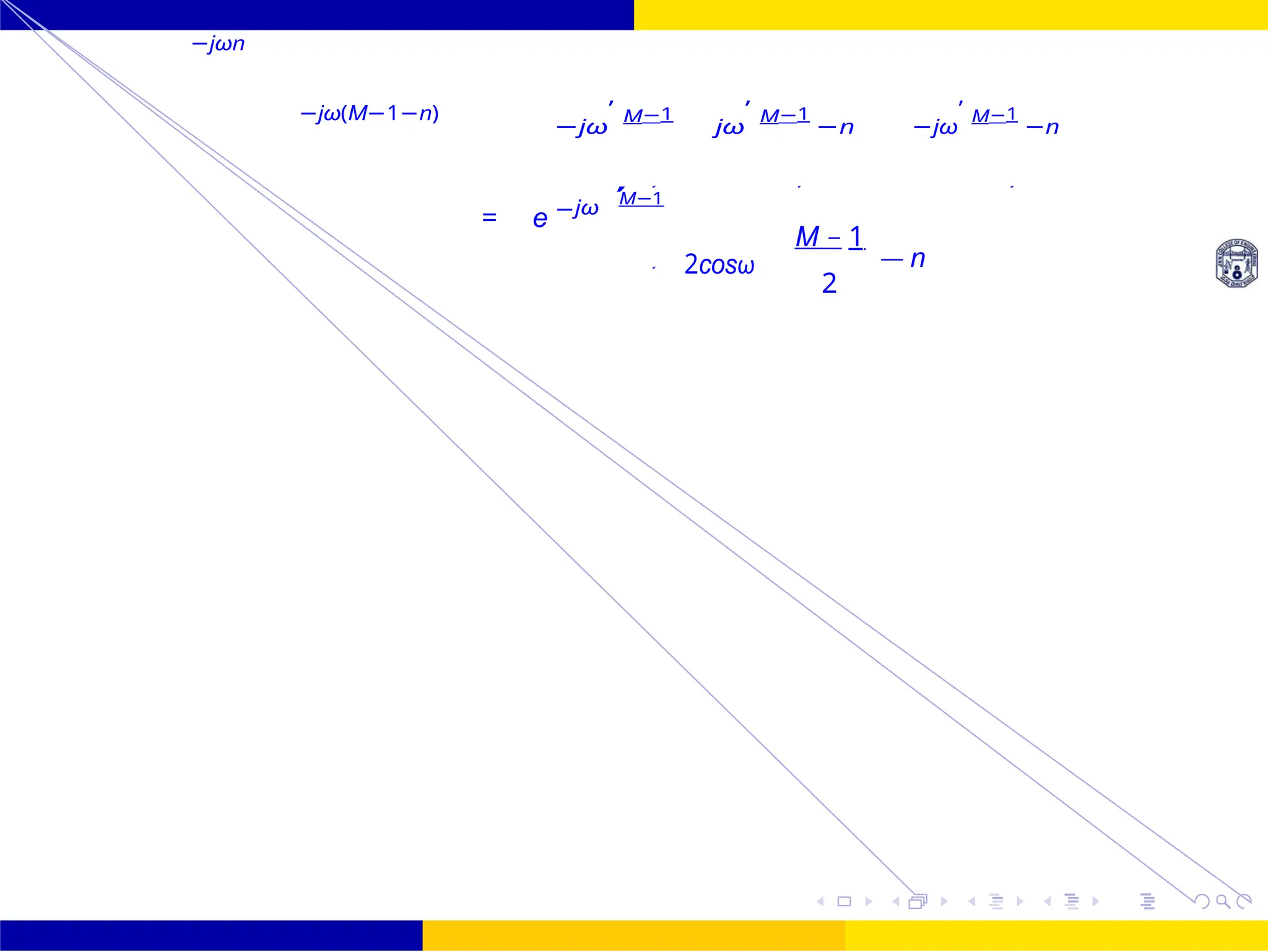
Frequency response of Linear Phase FIR Filter: Symmetric with M=odd
M−1
H(z ) = h(n)z −n
n=0
Symmetry: h(n)=h(M-1-n) Odd M
h[n]
Symmetric impulse response with M=odd Then
h(n) = h(M − 1 − n) and (z = ejω
)
H(z ) = h
M − 1
,
M−1
(M−3)/2
+
n=0
h(n)
h
z −n
+ z −(M−1−n)
i
H(ejω
) = h
M − 1
−jω
,
M−1
M−3
2
n=0
h(n)
h
e−jωn
+ e−jω(M−1−n)
i
−jωn
−jωn jω(
M−1
) −jω(
M−1
) jω(
M−1
−n) −jω(
M−1
)
e = e e 2
e
2 = e 2 .e 2
e−jω(M−1−n)
= e −jω(M−1)
ejωn
= e
−jω(
M−1
)
.e −jω(
M−1
) jωn −jω(
M−1
) −jω(
M−1
−n)
-2
-1
0
1
2
3
e +
z
2](https://image.slidesharecdn.com/dspmodule4ppt-241209183808-f5b6e07b/75/dsp-module-4-pptpptrpppptxppppppppp-docx-19-2048.jpg)
![2
Σ
2
2
Σ
2
Σ
2
Σ
∠H(ω) =
−ω + π for |H(ω)|
< 0
FIR Filter Design Symmetric and Antisymmetric FIR
Filters
21 /
October 25,
UNIT - 7: FIR Filter
H(ejω
) = h( M − 1
2
)e−jω( M−1
)
+
M−3
2
n=0
h(n)[e−jωn
+ e−jω(M−1−n)
]
= h
M − 1
−jω
,
M−1
M−3
2
n=0
h(n)e −jω
,
M−1
2cosω
M − 1
— n
2
= e
−jω
,
M−1
2
h
M − 1
2
M−3
2
+ 2
n=0
h(n)cos ω
M − 1
2
— n
H(ω) = |H(ω)|ej∠H(ω)
|H(ω)| = h
M − 1
+ 2
M−3
2
n=0
h(n)cos ω
M − 1
— n
2
e
+](https://image.slidesharecdn.com/dspmodule4ppt-241209183808-f5b6e07b/75/dsp-module-4-pptpptrpppptxppppppppp-docx-21-2048.jpg)
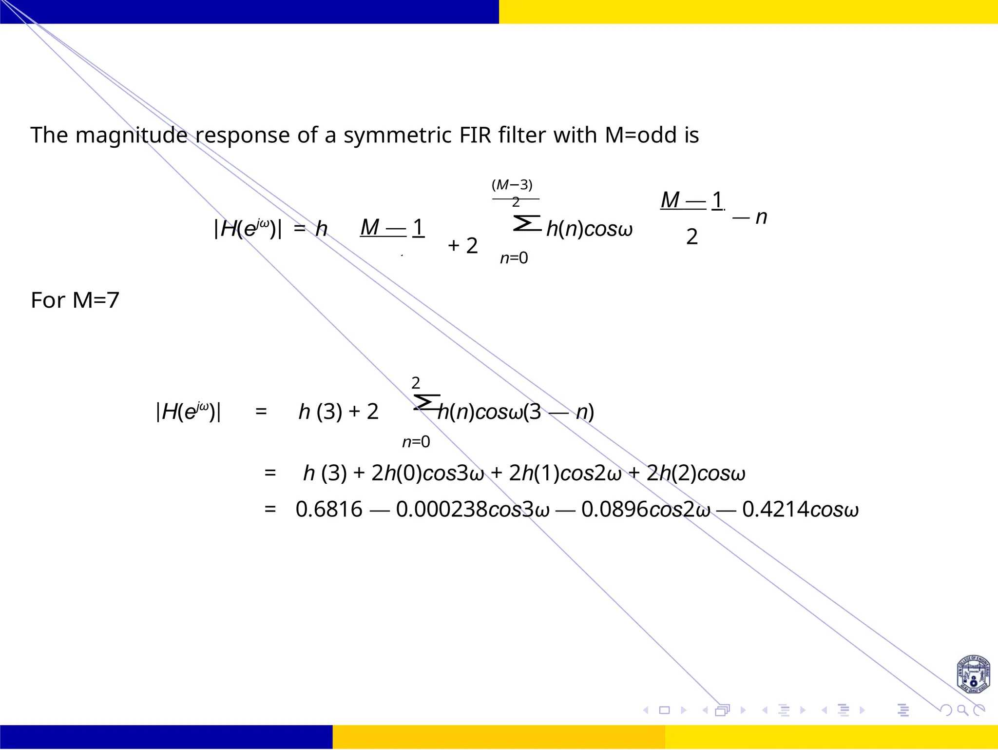
![
2
Σ
2
−ω for |H(ω)|
> 0
∠H(ω) =
−ω + π for |H(ω)|
< 0
FIR Filter Design Symmetric and Antisymmetric FIR
Filters
October 25, 23 /
UNIT - 7: FIR Filter
Frequency response of Linear Phase FIR Filter: Symmetric with M=Even
H(ω) = e
−jω
,
M−1
2
2
M
−1
n=0
h(n)cos ω
M − 1
2 — n
Symmetry: h(n)=h(M-1-n) Even M
h[n]
H(ω) = |H(ω)|ej∠H(ω)
|H(ω)| = 2
M
−1
n=0
h(n)cos ω
M − 1
— n
2
0 1 2 3 4 5 6 7 8 n
Center of Symmetry
M−1
2
M−1
2
-2
-1
0
1
2
3
Σ](https://image.slidesharecdn.com/dspmodule4ppt-241209183808-f5b6e07b/75/dsp-module-4-pptpptrpppptxppppppppp-docx-23-2048.jpg)


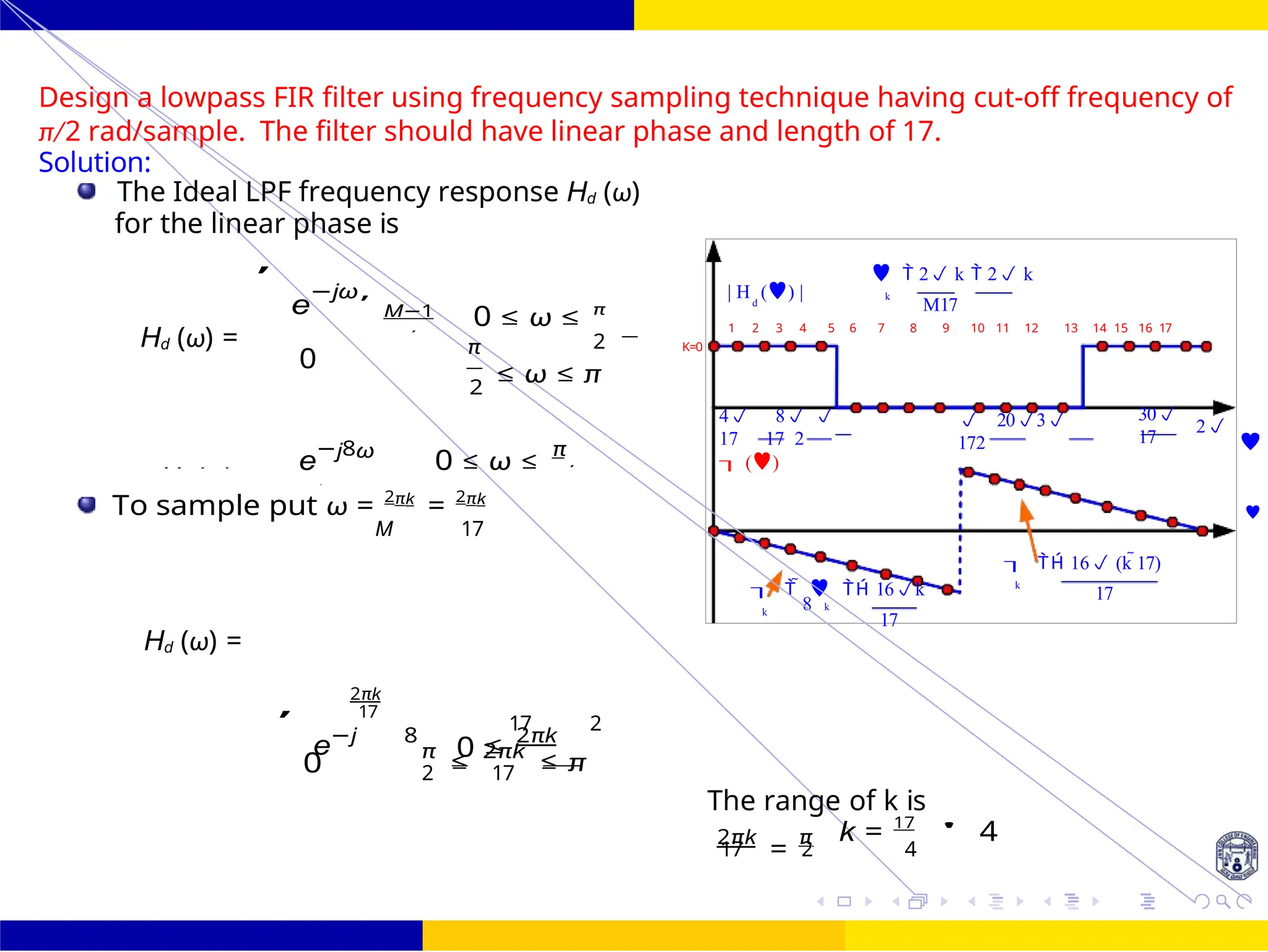
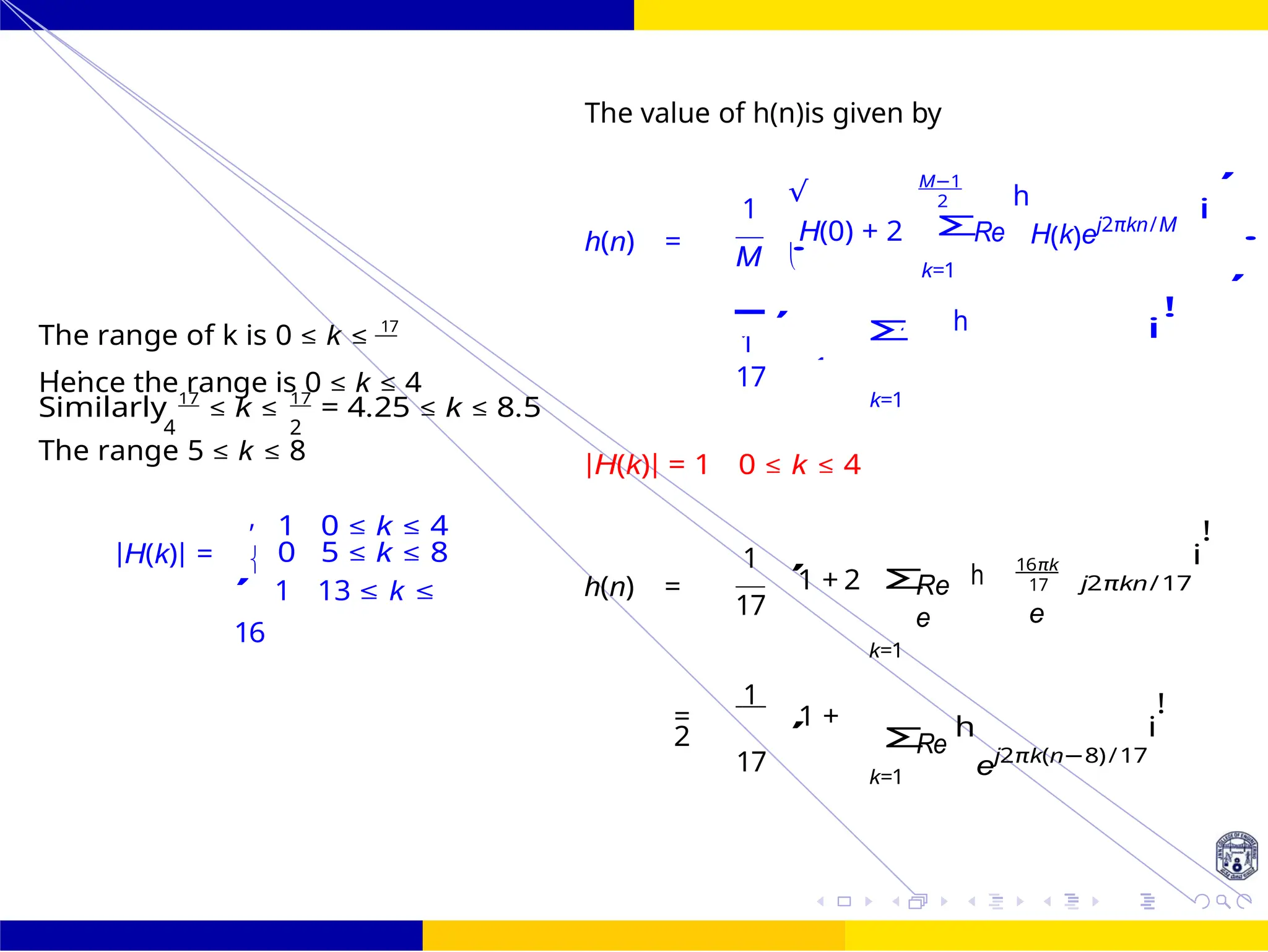
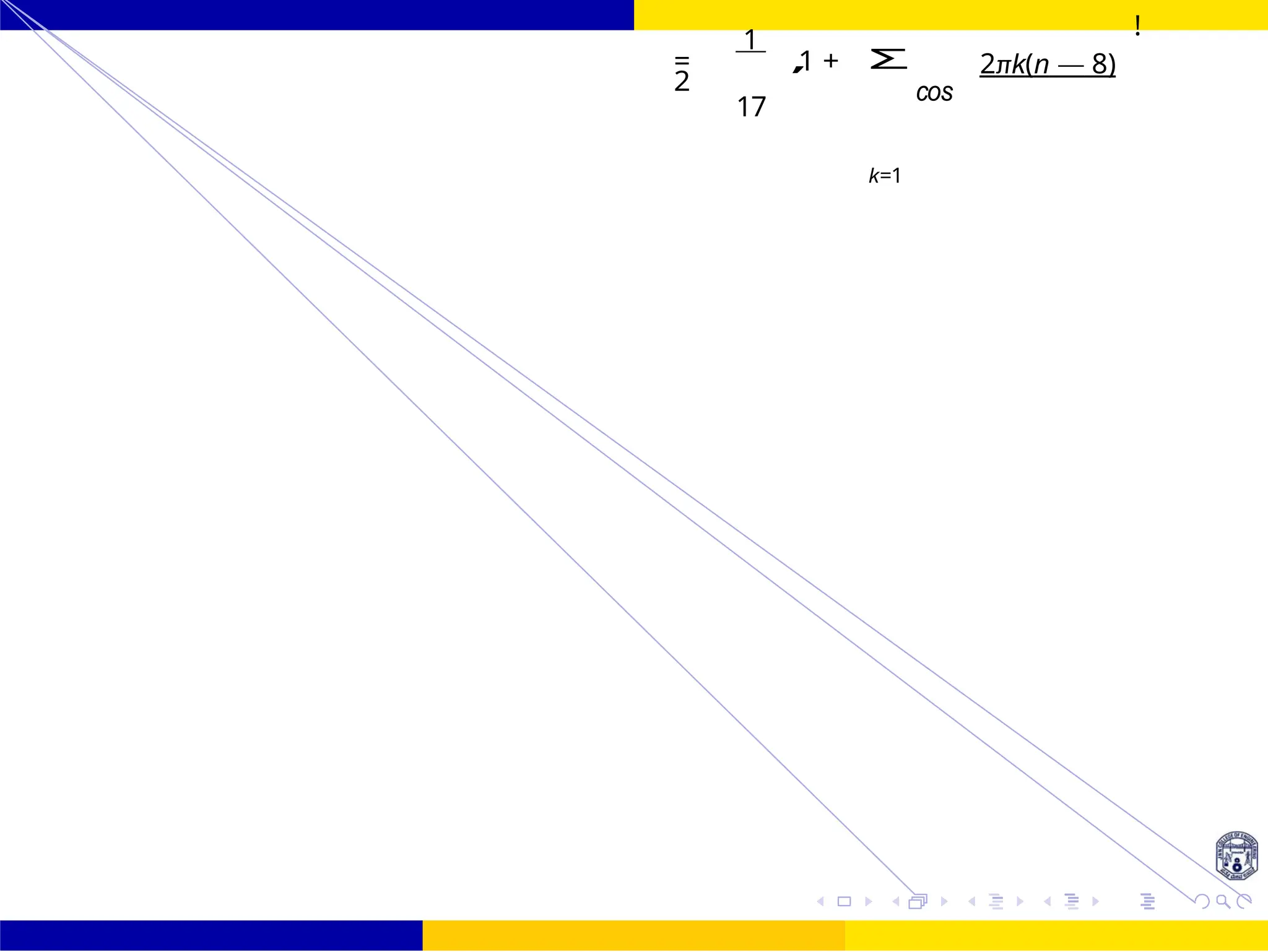
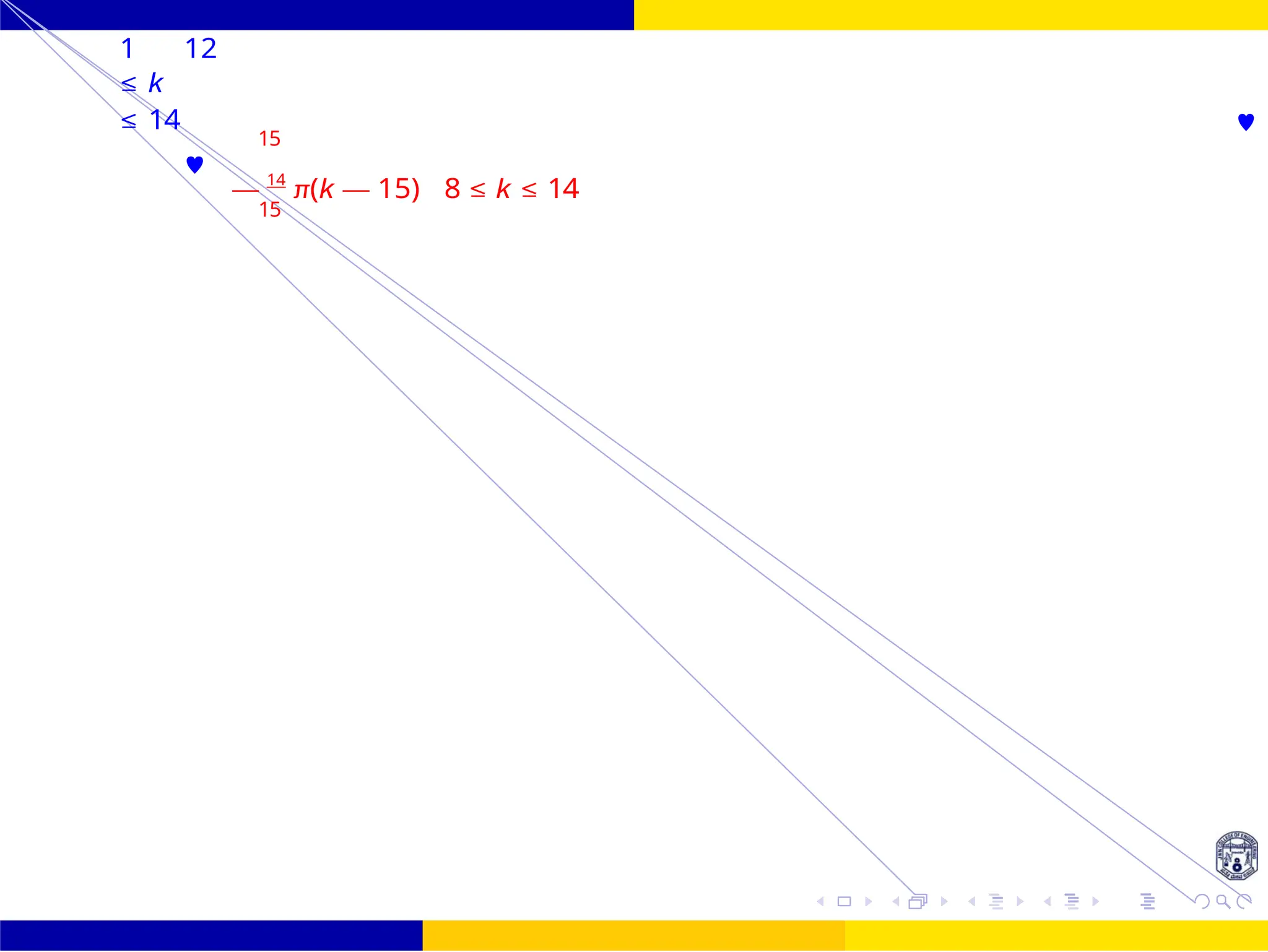
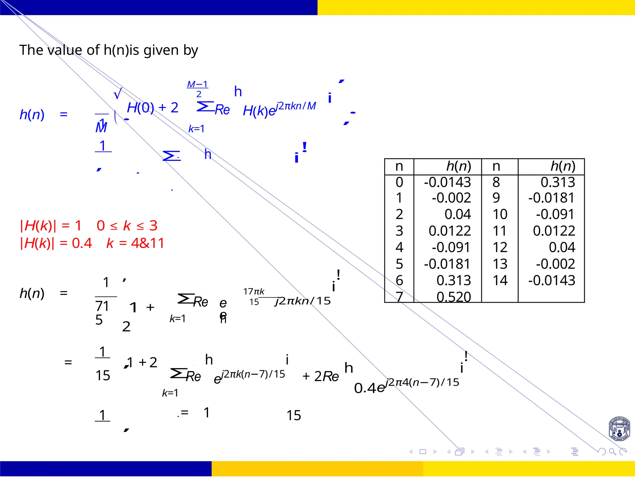
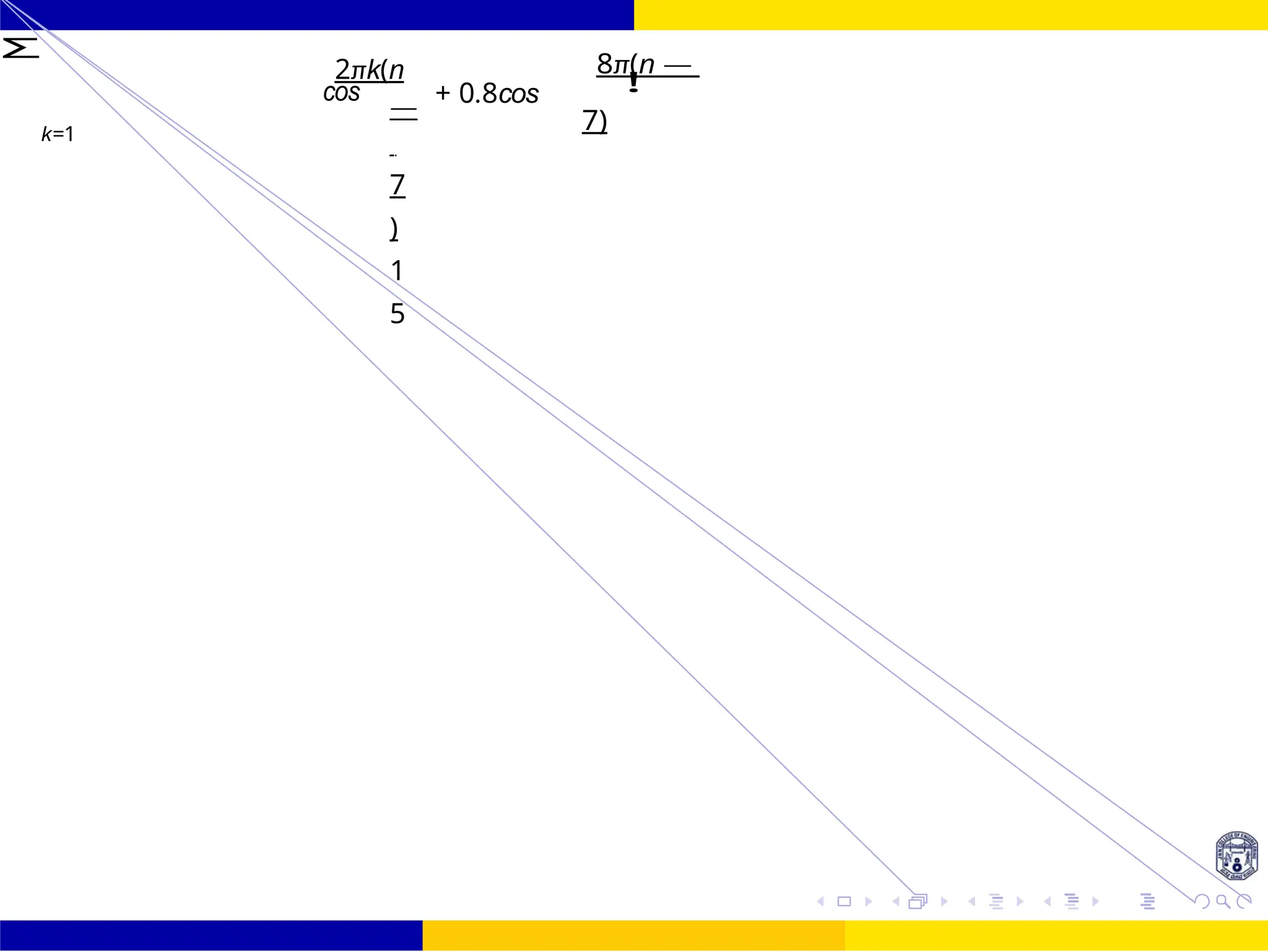
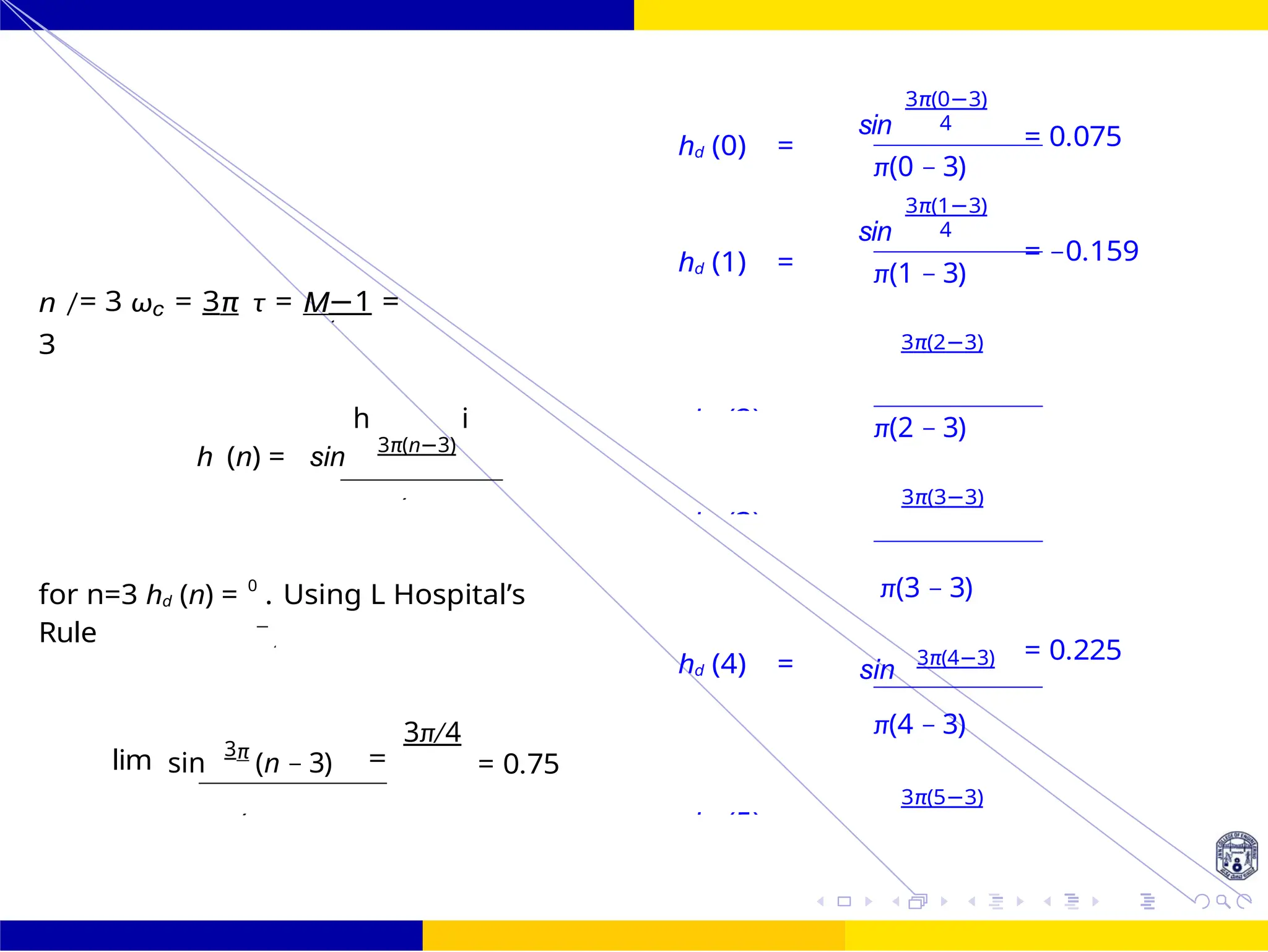
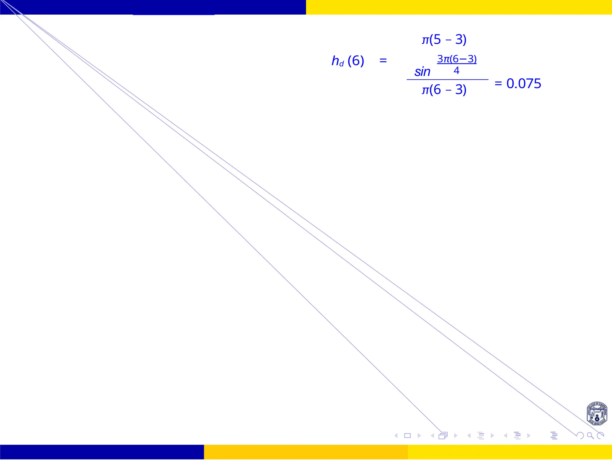
![2
0
FIR Filter Design Low Pass FIR Filter
Design
October 25, 30 /
UNIT - 7: FIR Filter
h (n) =
sin [ωc (n − τ )]
π(2−5)
d
π(n − τ )
for n /= 5 and ωc = π , τ = M−1 =
5
sin
hd (2) = 2
π(2 − 5)
π(3−5)
= −0.106
2 2
hd (3) = sin 2
= 0
h (n) =
sin [ωc (n − 5)]
=
sin
h
π(n−5)
i π(3 − 5)
sin
π(4−5)
d
π(n − 5) π(n − 5) hd (4) =
2
= .318
π(4 − 5)
for n=5 hd (n) = 0
. Using L Hospital’s Rule
sin Bθ
lim = B
hd (5) =
sin
π(5−5)
2
= .5
π(5 − 5)
sin
π(6−5)
θ→0 θ hd (6) =
2
= .318
π(6 − 5)
sin π
(n − 5)
lim 2
= π/2
= 0.5 hd (7) =
sin
π(7−5)
2
= 0.0
n→5 π(n − 5) π π(7 − 5)
where π = 3.1416
hd (0) = sin
π(0−5)
2
= 0.0637
π(0 − 5)
hd (8) =](https://image.slidesharecdn.com/dspmodule4ppt-241209183808-f5b6e07b/75/dsp-module-4-pptpptrpppptxppppppppp-docx-46-2048.jpg)
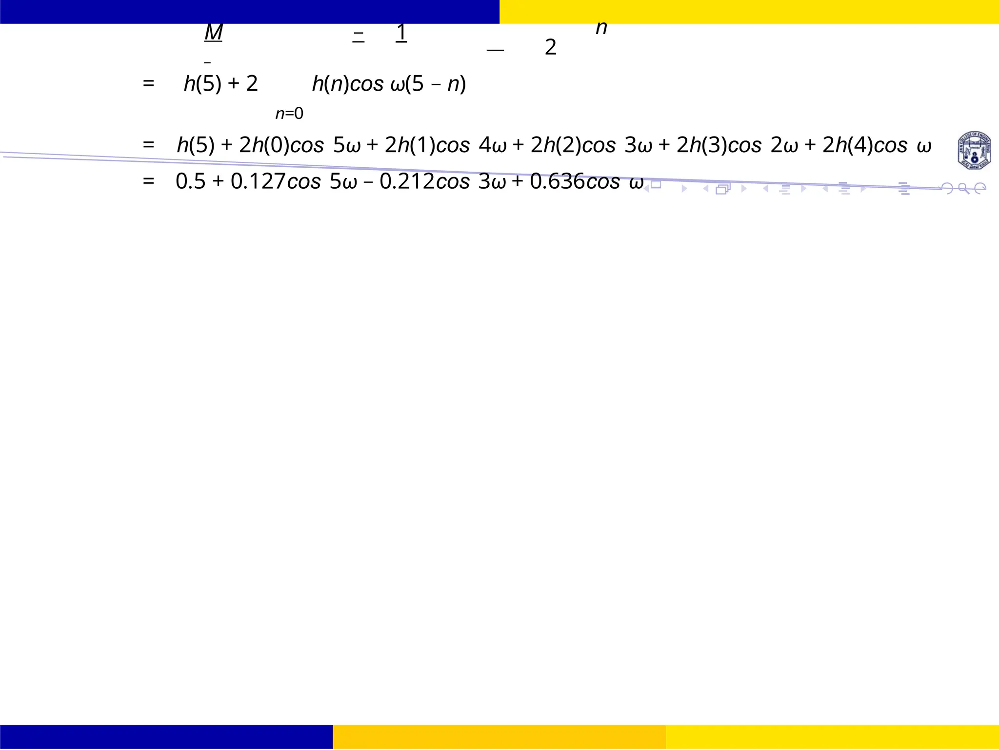
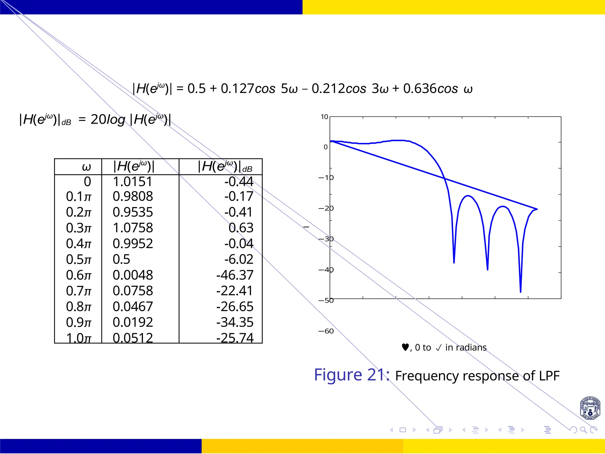
![Σ
Σ
Σ
FIR Filter Design Low Pass FIR Filter
Design
32 /
October 25,
UNIT - 7: FIR Filter
The given window is rectangular window
ω(n) =
1 for 0 ≤ n ≤ 10
0 Otherwise
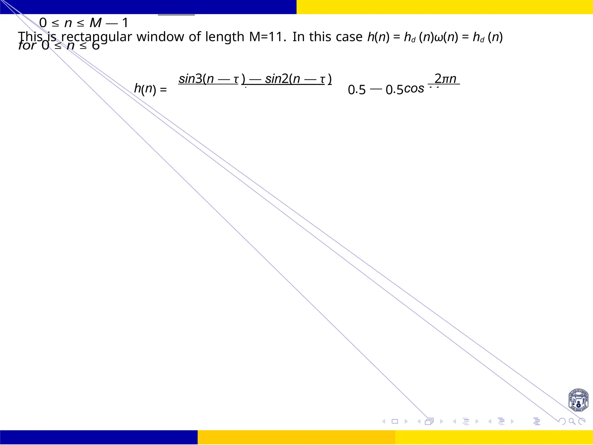
This is rectangular window of length M=11. h(n) = hd (n)ω(n) = hd (n) for 0 ≤ n ≤ 10
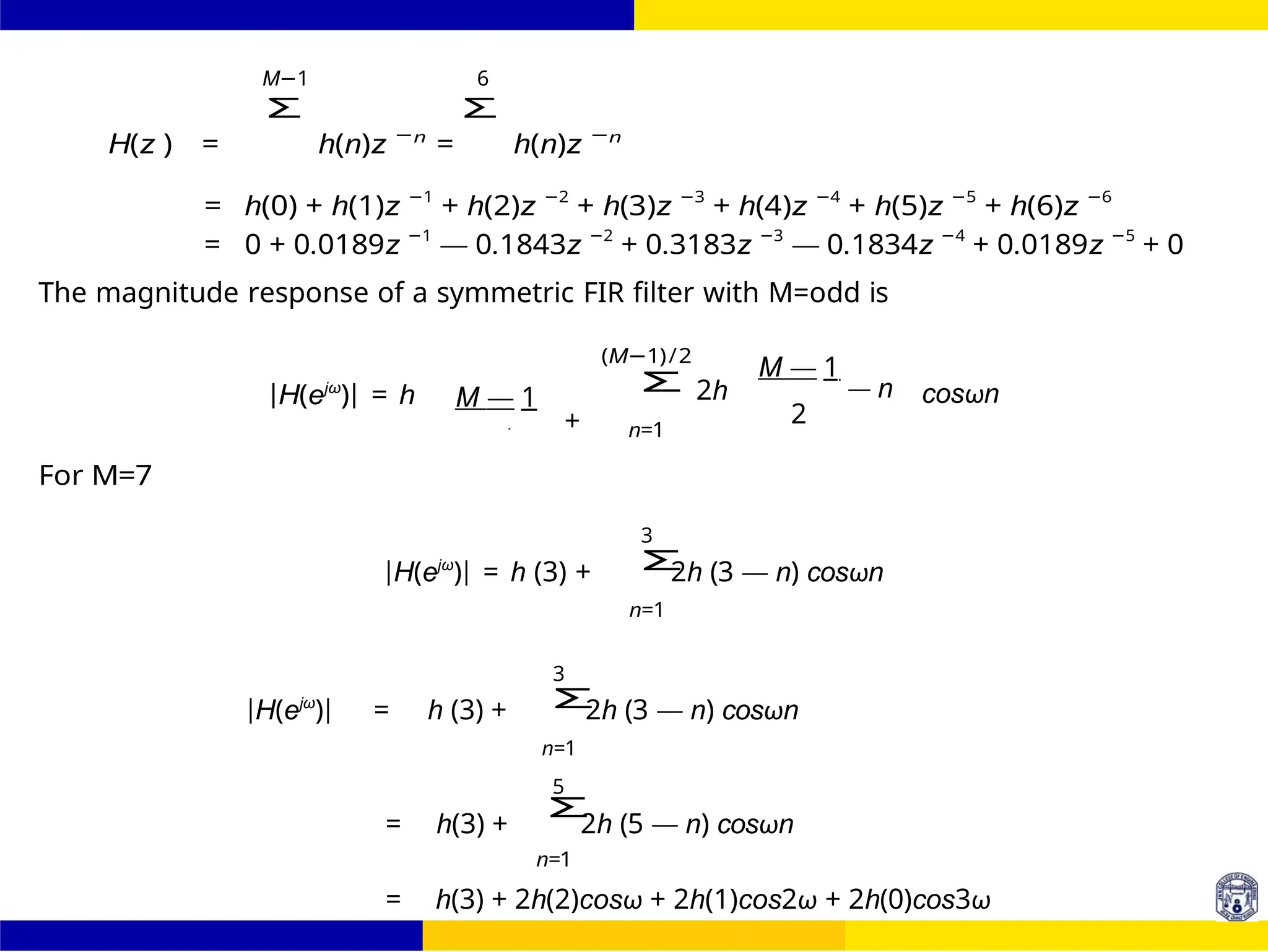
M−1 10
H(z ) =
Σ
h(n)z −n
=
Σ
h(n)z −n
n=0 n=0
The impulse response is symmetric with M=odd=11
H(z ) = h
M − 1
z
M−3
2 +
M−3
2
n=0
h(n)[z −n
+ z (M−1−n)
]
= h(5)z −5
+ h(0)[z −0
+ z −10
] + h(1)[z −1
+ z −9
] + h(2)[z −2
+ z −8
] +
= +h(3)[z −3
+ z −7
] + h(4)[z −4
+ z −6
]
|H(ejω
)| = h
M − 1
+ 2
4
M−3 2
n=0
h(n)cos ω
2
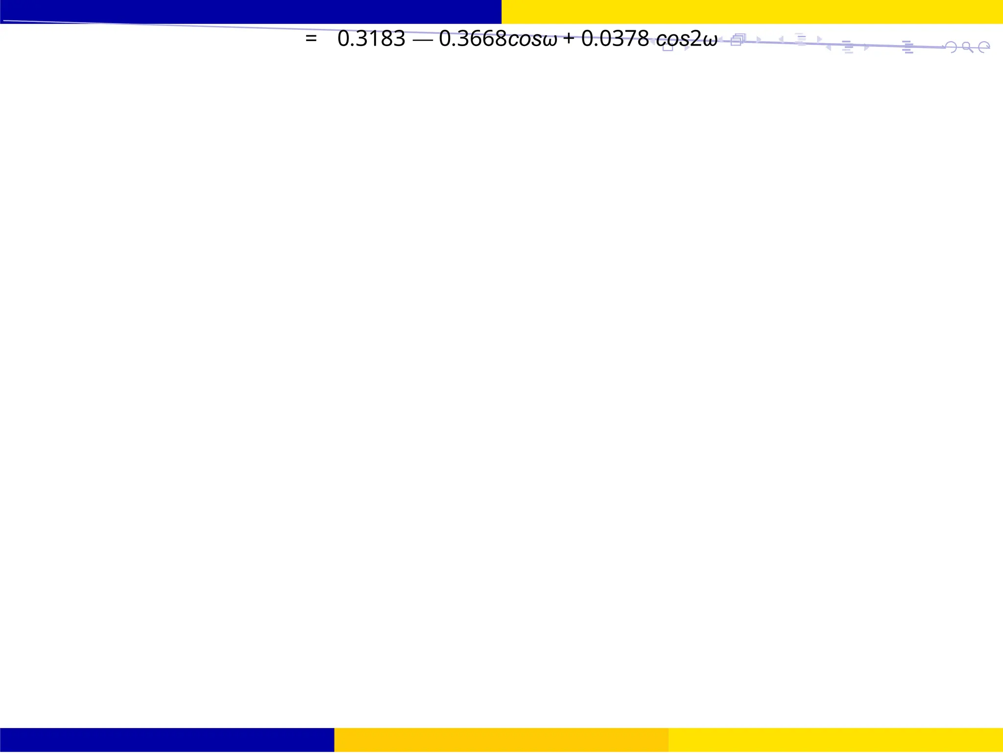
2](https://image.slidesharecdn.com/dspmodule4ppt-241209183808-f5b6e07b/75/dsp-module-4-pptpptrpppptxppppppppp-docx-48-2048.jpg)


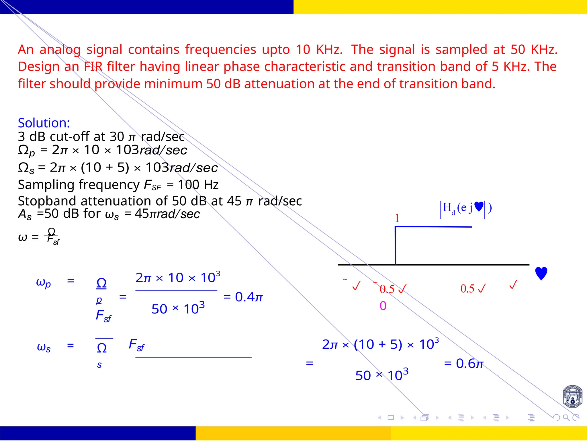
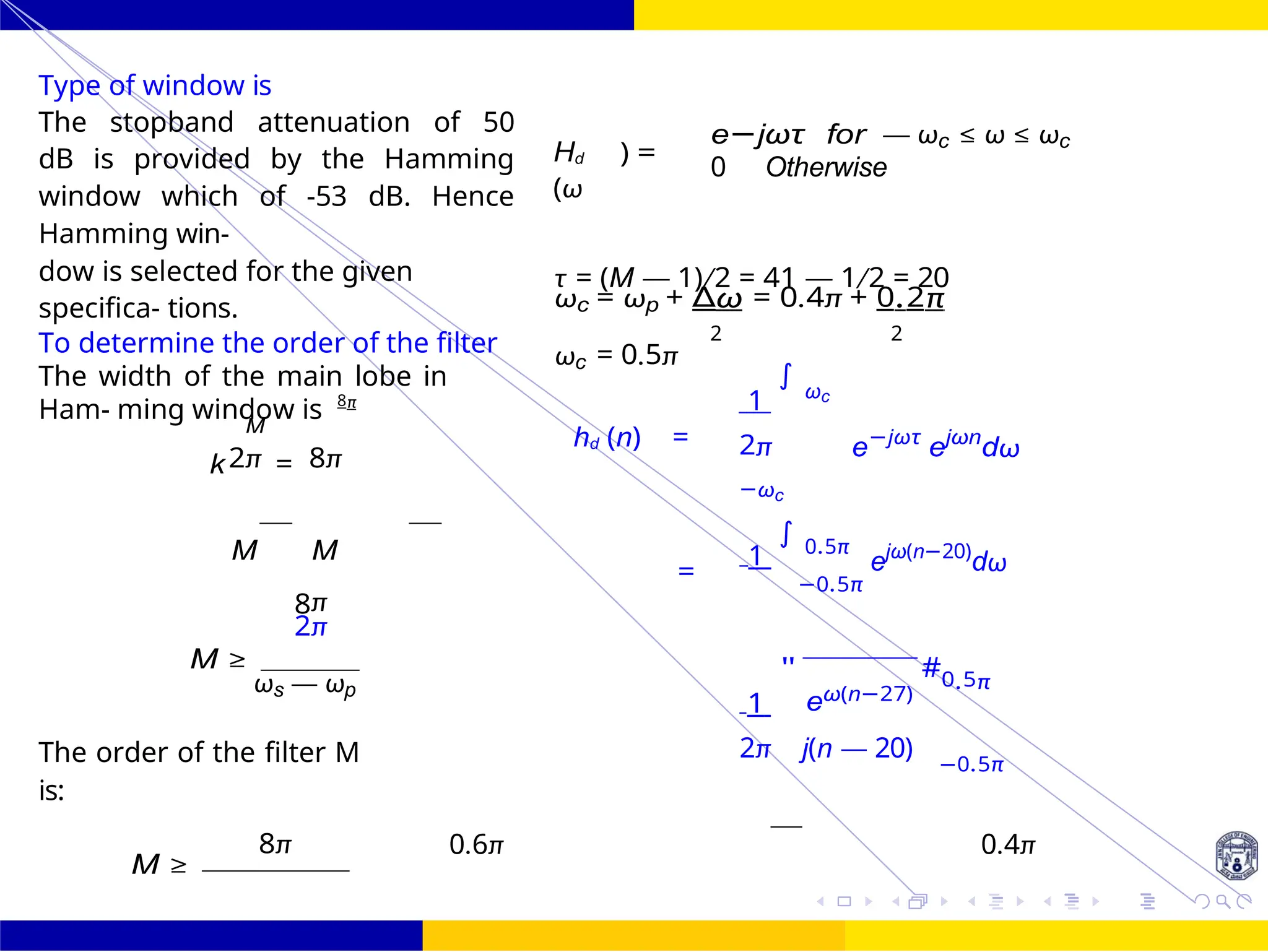
![FIR Filter Design Low Pass FIR Filter
Design
59 /
October 25,
UNIT - 7: FIR Filter
Dr. Manjunatha. P (JNNCE)
= 53.33 =
sin
(n
27)]
π(n — 27)
when n = 27
for n /= 27
Assume linear phase FIR filter of
odd
length Hence select next odd
integer
h (n) =
ωc
= 0.3
d
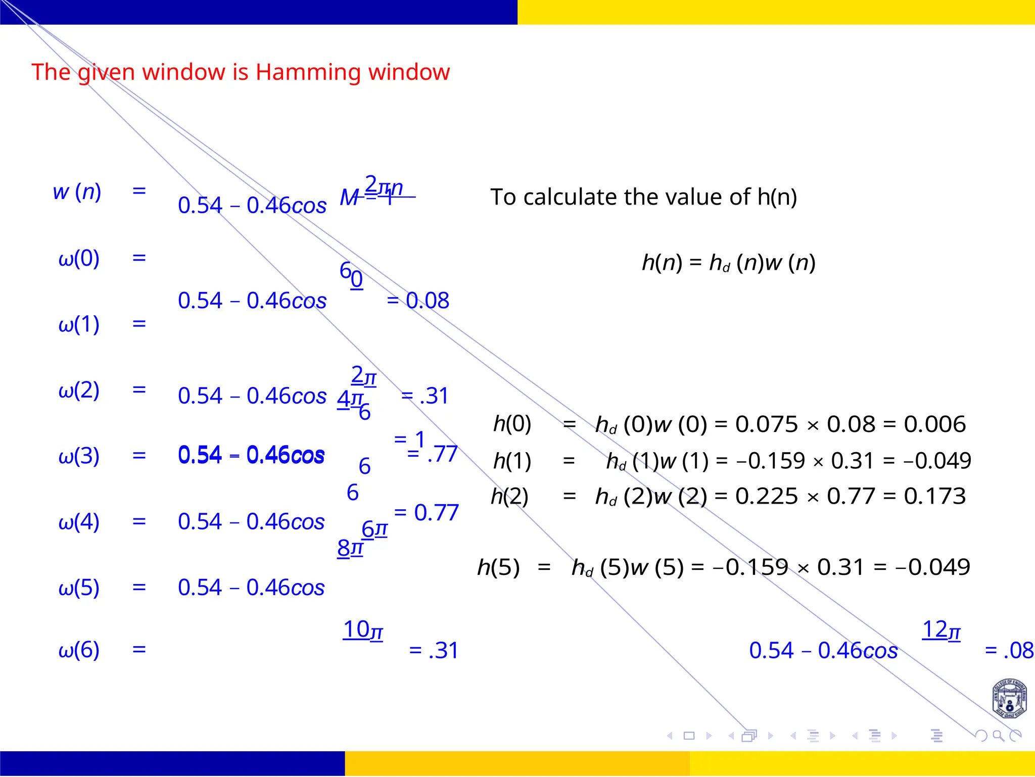
length of 55. π](https://image.slidesharecdn.com/dspmodule4ppt-241209183808-f5b6e07b/75/dsp-module-4-pptpptrpppptxppppppppp-docx-75-2048.jpg)
![M
FIR Filter Design Low Pass FIR Filter
Design
60 /
October 25,
UNIT - 7: FIR Filter
Dr. Manjunatha. P (JNNCE)
The selected window is Hamming M=27
2πn
= 0.54 — 0.46cos
πn
18
The value of h(n)
h(n) = hd (n)w (n)
for M= 27
h(n) =
sin[0.3π(n — 27)]
π(n — 27) 0.54 —
0.46cos
πn i
for n /= 27 h
(n
) = 0.3
h
w (n) = 0.54 —
n h(n) n h(n)
0 0.0 28 0.2567
1 0.0 29 0.1495
2 -0.0012 30 0.0319
3 0.0 31 -0.0445
4 0.0 32 -0.0588
5 0.0021 33 - 0.0278
6 0.0023 34 0.012
7 0.0 35 0.0308
8 -0.0036 36 0.0220
9 -0.0052 37 -0.0
10 -0.0021 38 -0.0157
11 0.0048 39 -0.0156
12 0.0098 40 -0.0043
13 0.0069 41 0.0069
14 -0.0043 42 0.0098
15 -0.0156 43 0.0048
16 -0.0157 44 -0.0021
17 0.0 45 -0.0052
18 0.0220 46 -0.0036
19 -0.0308 47 0.0
20 -0.0120 48 0.0023
21 -0.0278 49 0.0021
22 -0.0588 50 0.0
23 -0.0445 51 0.0
24 0.0319 52 -0.0012
25 0.1495 53 0.0
26 0.2567 54 0.0
27 0.3
1](https://image.slidesharecdn.com/dspmodule4ppt-241209183808-f5b6e07b/75/dsp-module-4-pptpptrpppptxppppppppp-docx-76-2048.jpg)
![FIR Filter Design Low Pass FIR Filter
Design
October 25, 65 /
UNIT - 7: FIR Filter
Dr. Manjunatha. P (JNNCE)
≥ 40 =
si
n[ωc (n — 20)]
for n /= 20
π(n — 20)
Assume linear phase FIR filter of
odd length Hence select next odd
integer length of 41.
when n = 20
hd (n) =
ωc
=
π
0.5π
= 0.5
π](https://image.slidesharecdn.com/dspmodule4ppt-241209183808-f5b6e07b/75/dsp-module-4-pptpptrpppptxppppppppp-docx-81-2048.jpg)
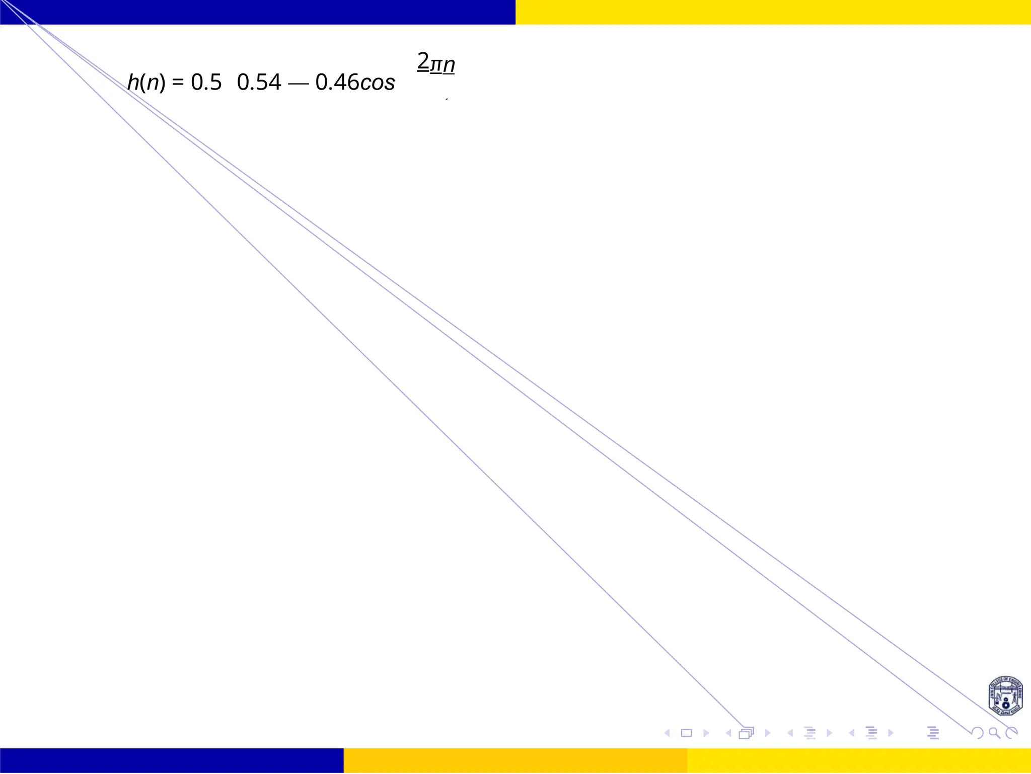
![FIR Filter Design Low Pass FIR Filter
Design
66 /
October 25,
UNIT - 7: FIR Filter
Dr. Manjunatha. P (JNNCE)
M
2
The selected window is Hamming M=41
2πn
= 0.54 — 0.46cos
2πn
40
The value of h(n)
h(n) = hd (n)w (n)
for M= 41 n /= 20
h(n) =
sin[0.5π(n — 20)]
π(n — 20) 0.54 —
0.46cos
2πn
for n = 20
w (n) = 0.54 —
n h(n) n h(n)
0 0.0 21 0.3148
1 -0.00146 22 0.0
2 0.0 23 -0.1
3 -0.00247 24 0.0
4 0 25 0.055
5 -0.00451 26 0.0
6 0.0 27 -0.0337
7 0.0079 28 0.0
8 0.0 29 0.0213
9 -0.0136 30 0.0
10 0.0 31 -0.0136
11 0.002135 32 0.0
12 0.0 33 0.0079
13 -0.03375 34 0
14 0.0 35 -0.0045
15 0.05504 36 0.0
16 0.0 37 0.0024
17 -0.1006 38 0.0
18 0.0 39 -0.0014
19 0.3148 40 0.0
20 0.5](https://image.slidesharecdn.com/dspmodule4ppt-241209183808-f5b6e07b/75/dsp-module-4-pptpptrpppptxppppppppp-docx-82-2048.jpg)
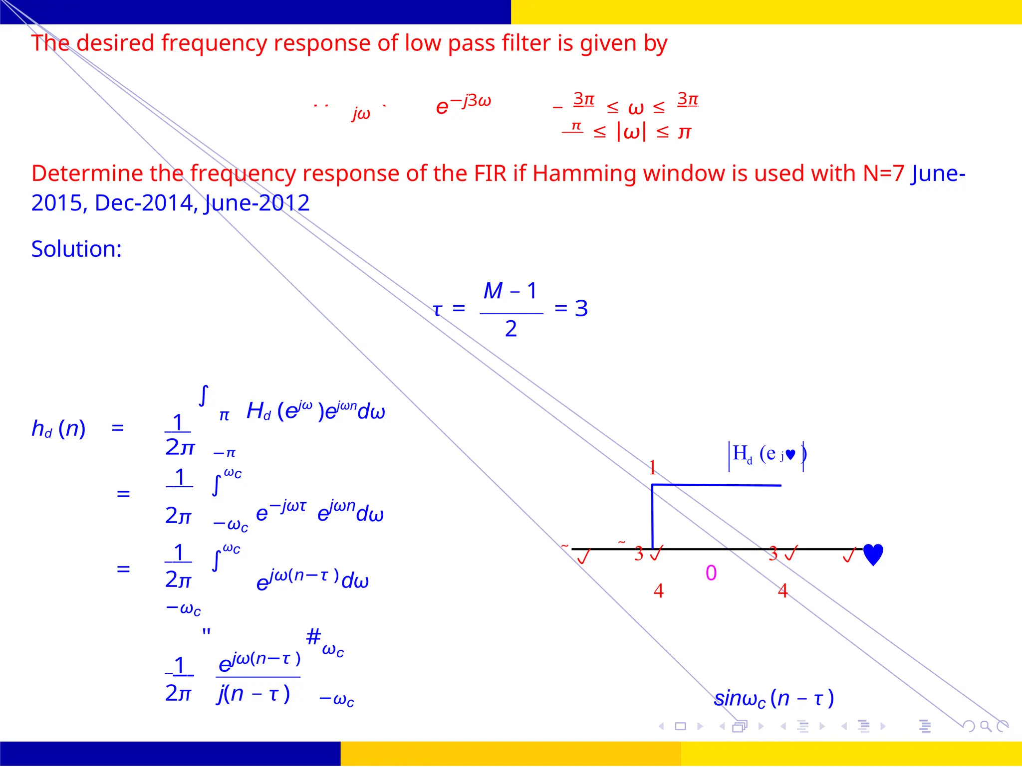
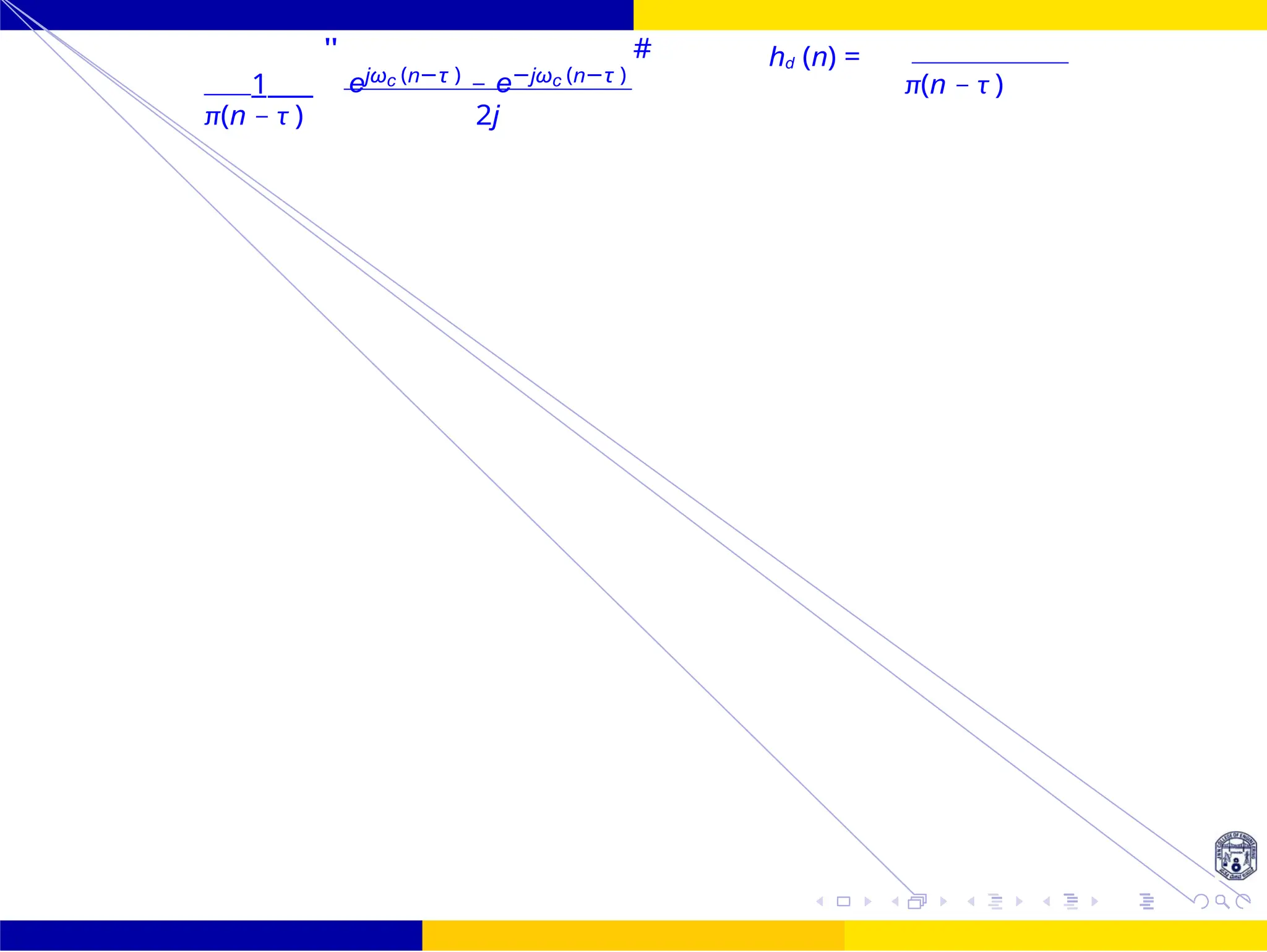
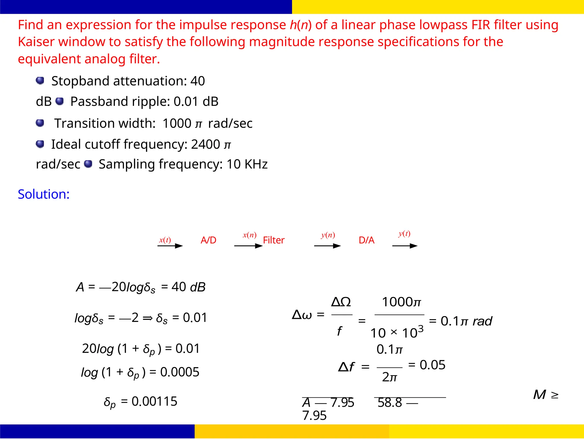
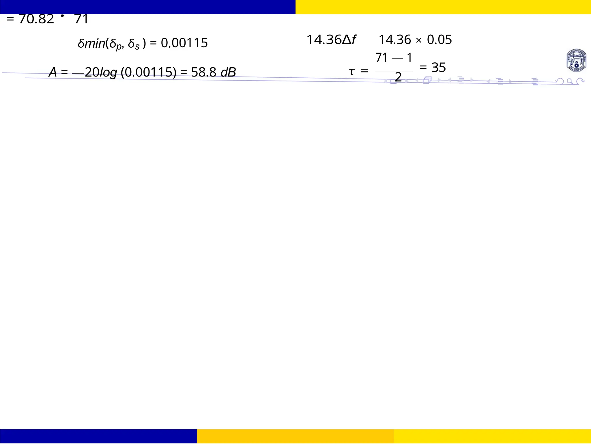
![F
∫
1
"
eω(n−3)
∫
FIR Filter Design Low Pass FIR Filter
Design
Dr. Manjunatha. P (JNNCE) October 25, 68 /
UNIT - 7: FIR Filter
1
H (e j )
d
Design an FIR filter (lowpass) using rectangular window with passband gain of 0 dB, cutoff
frequency of 200 Hz, sampling frequency of 1 kHz. Assume the length of the impulse
response as 7.
Solution:
Fc = 200 Hz, Fs = 1000 Hz,
fc = Fc 200
= 0.2cycles/sample
s
ωc = 2π ∗ fc = 2π × 0.2 = 0.4πrad
M=7
Hd (ω) = e−jωτ for — ωc ≤ ω ≤ ωc
0 Otherwise
0.4
0
0.4
τ = (M — 1)/2 = 7 — 1/2 = 3
ωc = 0.4π
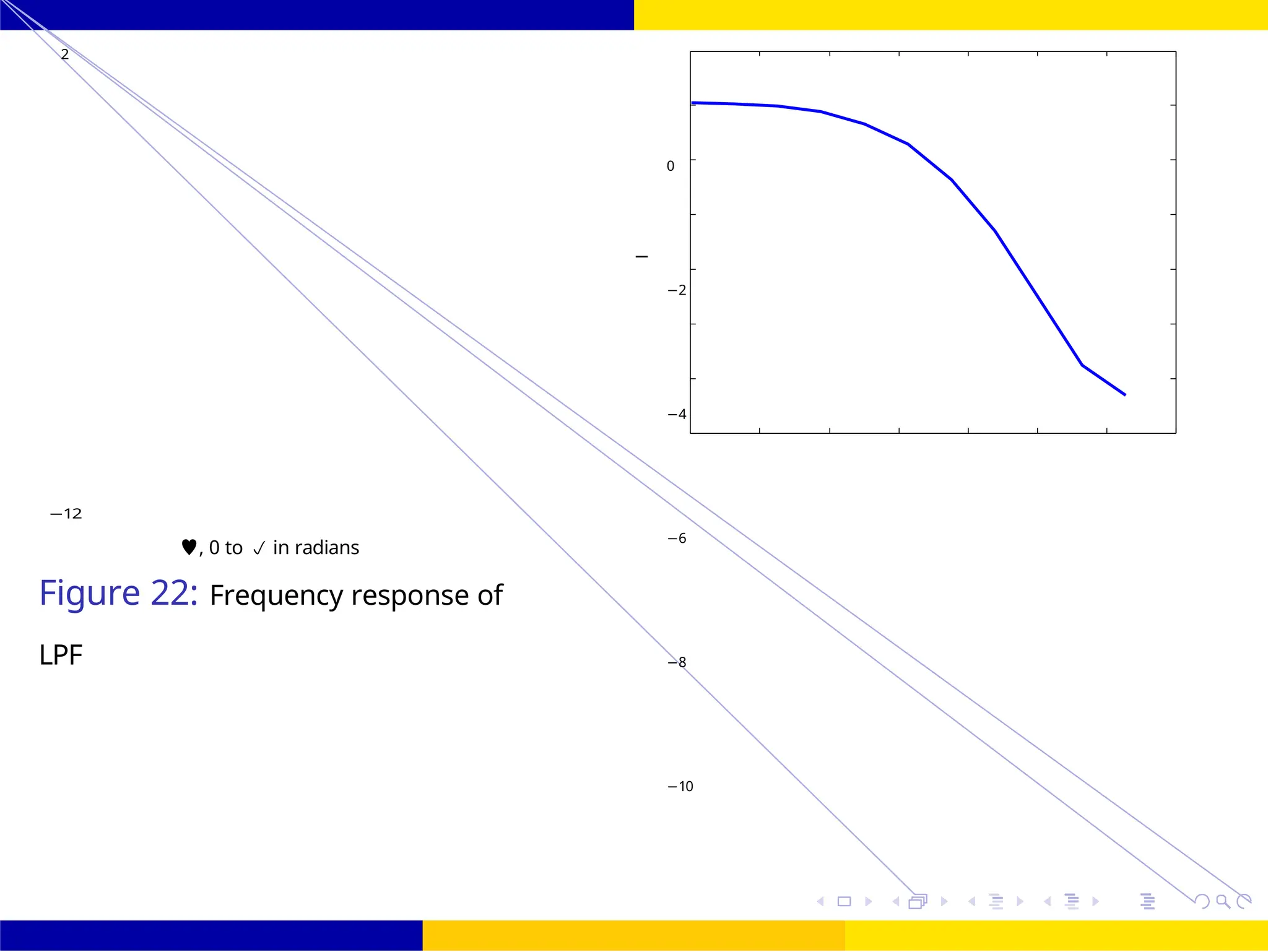
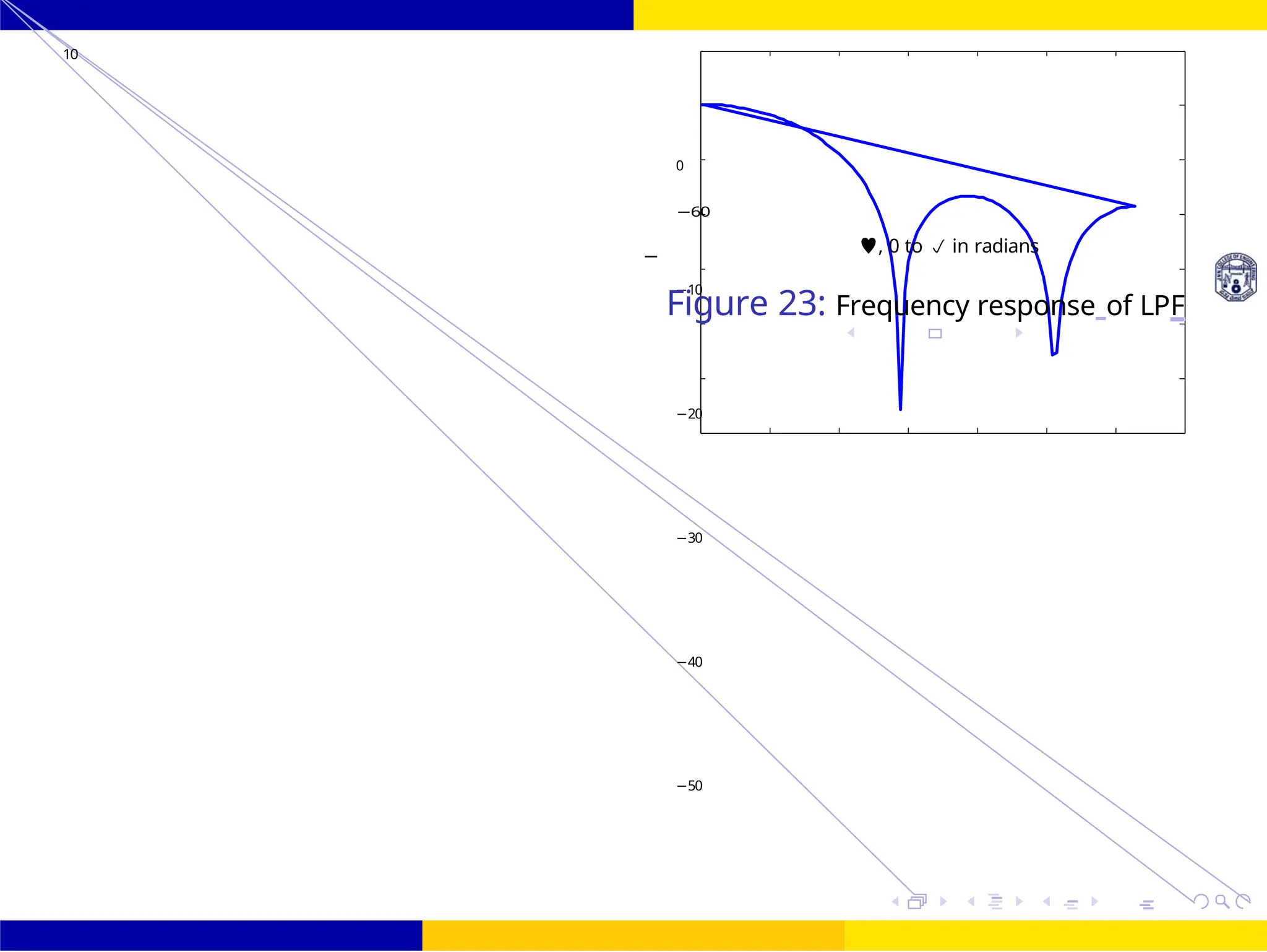
Figure 27: Frequency response of LPF
when n /= 3
hd (n) = 1 ωc
2π
−ωc
e−jωτ
ejωn
dω
h (n) = sin[0.4π(n — 3)]
1 0.4π
=
2π −0.4π
ejω(n−3)
dω
d
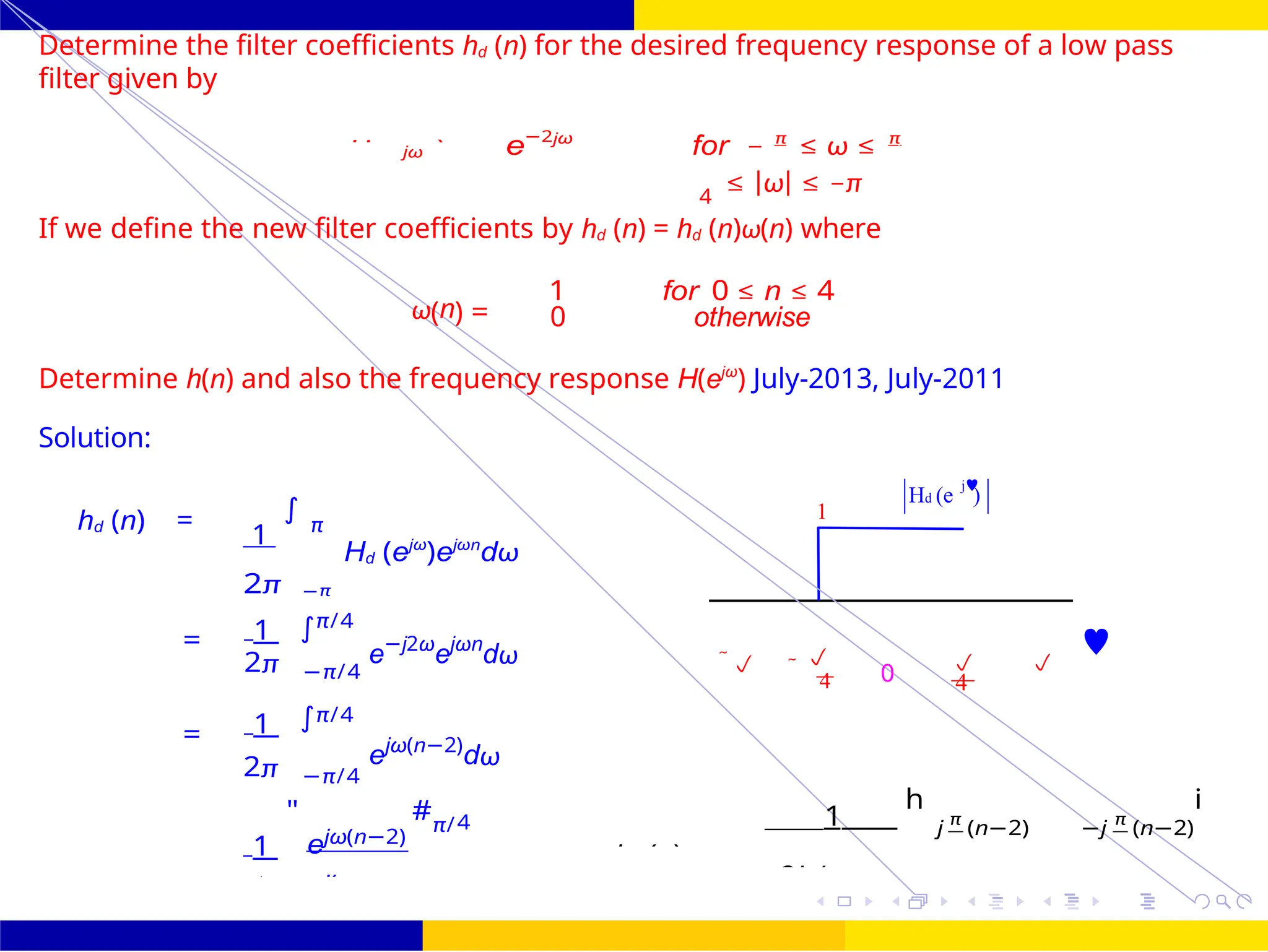
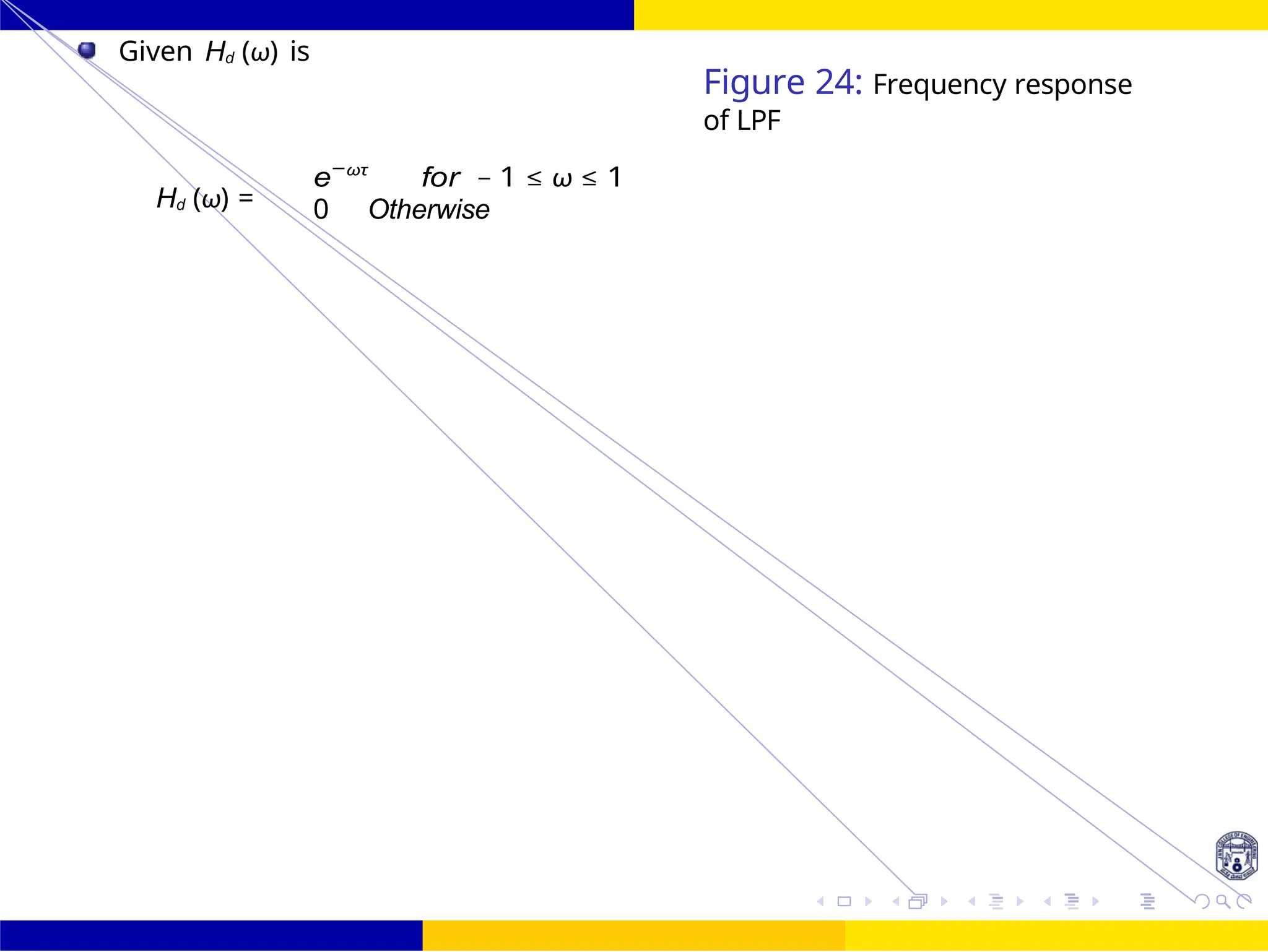
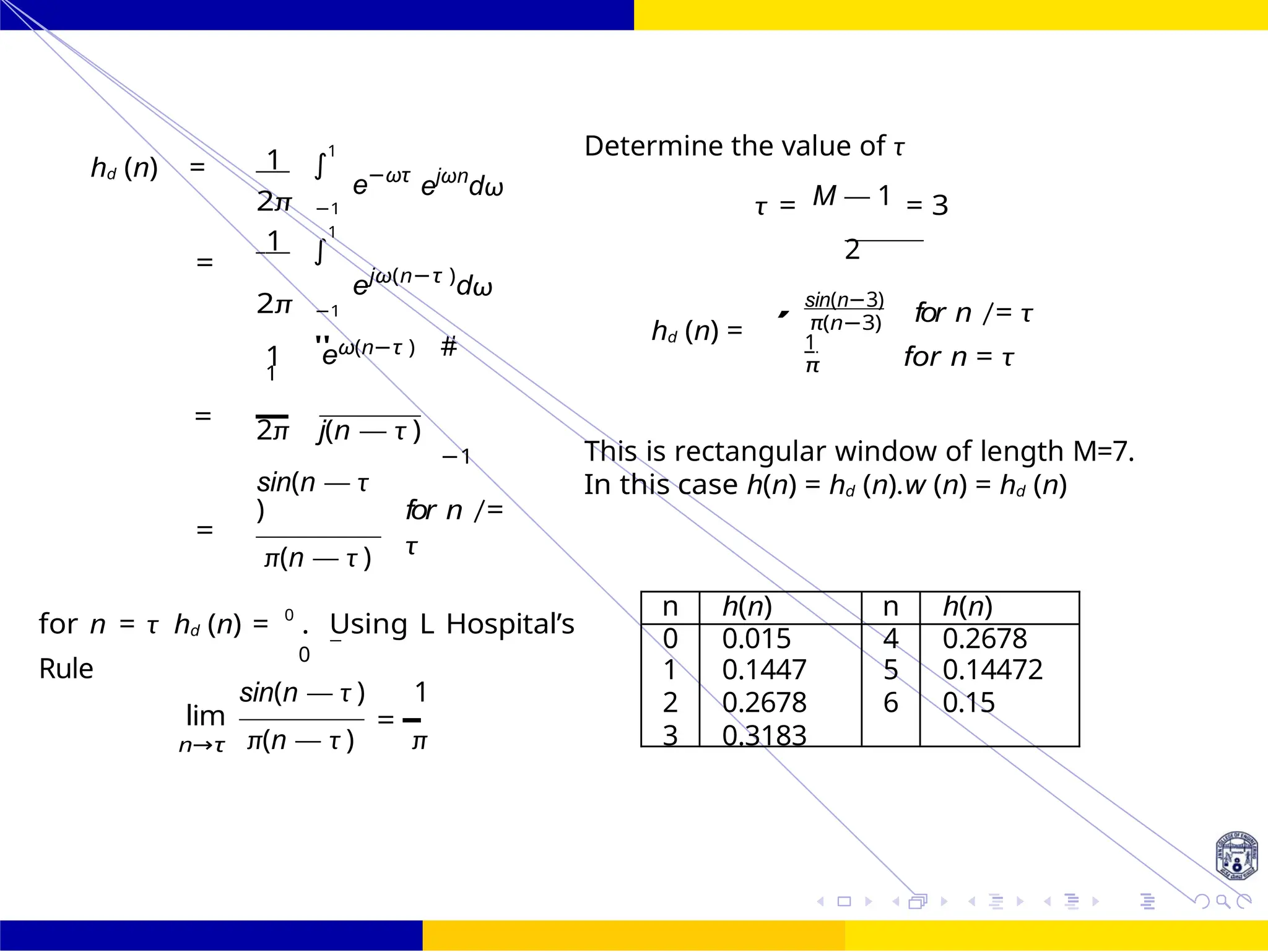
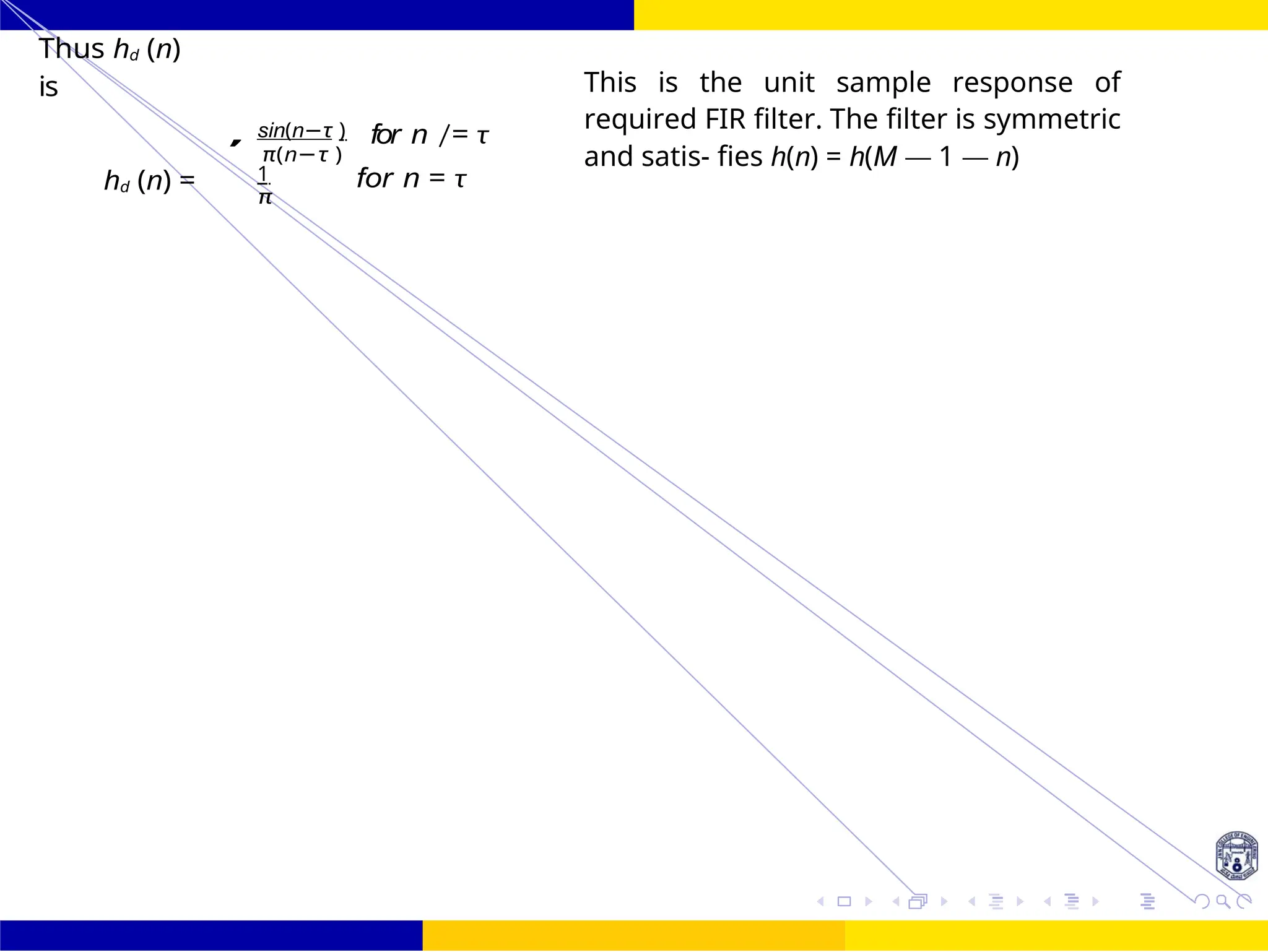
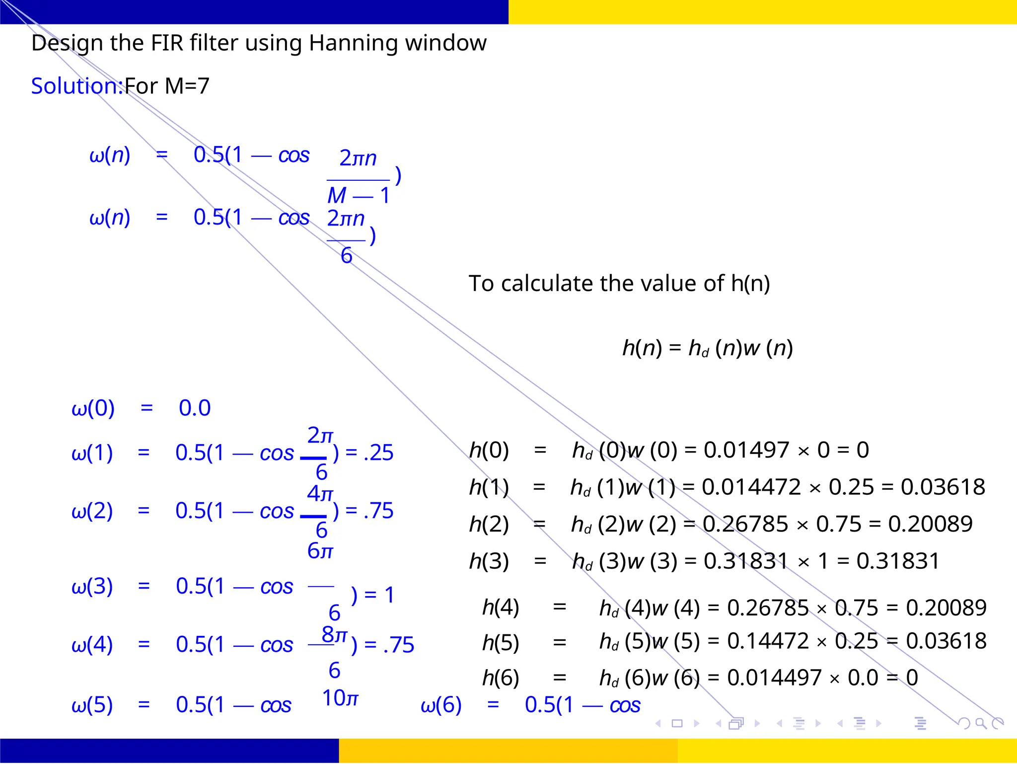
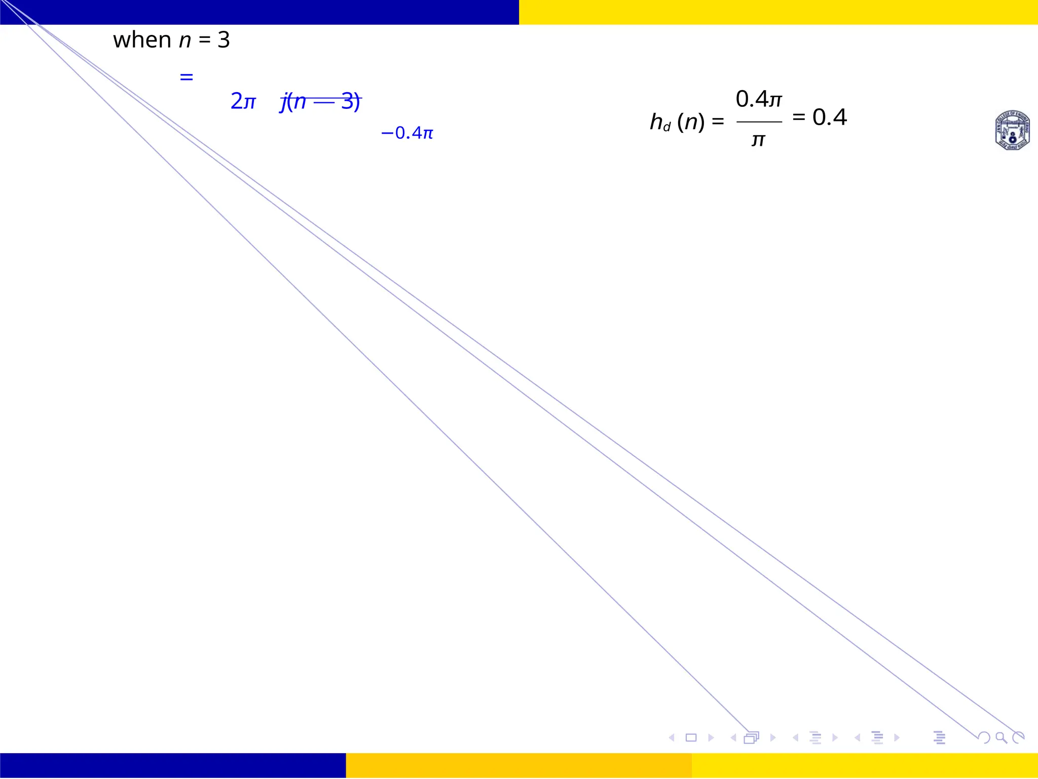
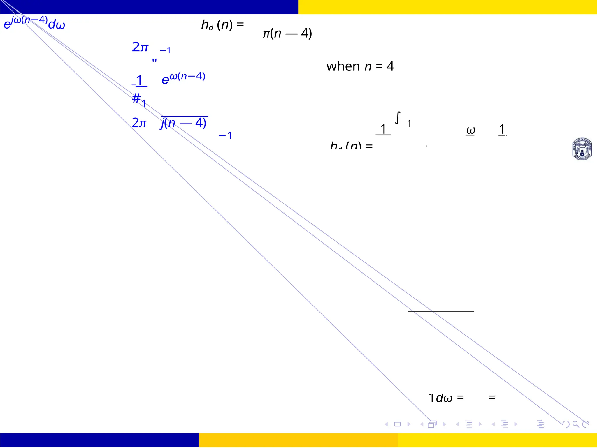
π(n — 3)](https://image.slidesharecdn.com/dspmodule4ppt-241209183808-f5b6e07b/75/dsp-module-4-pptpptrpppptxppppppppp-docx-84-2048.jpg)
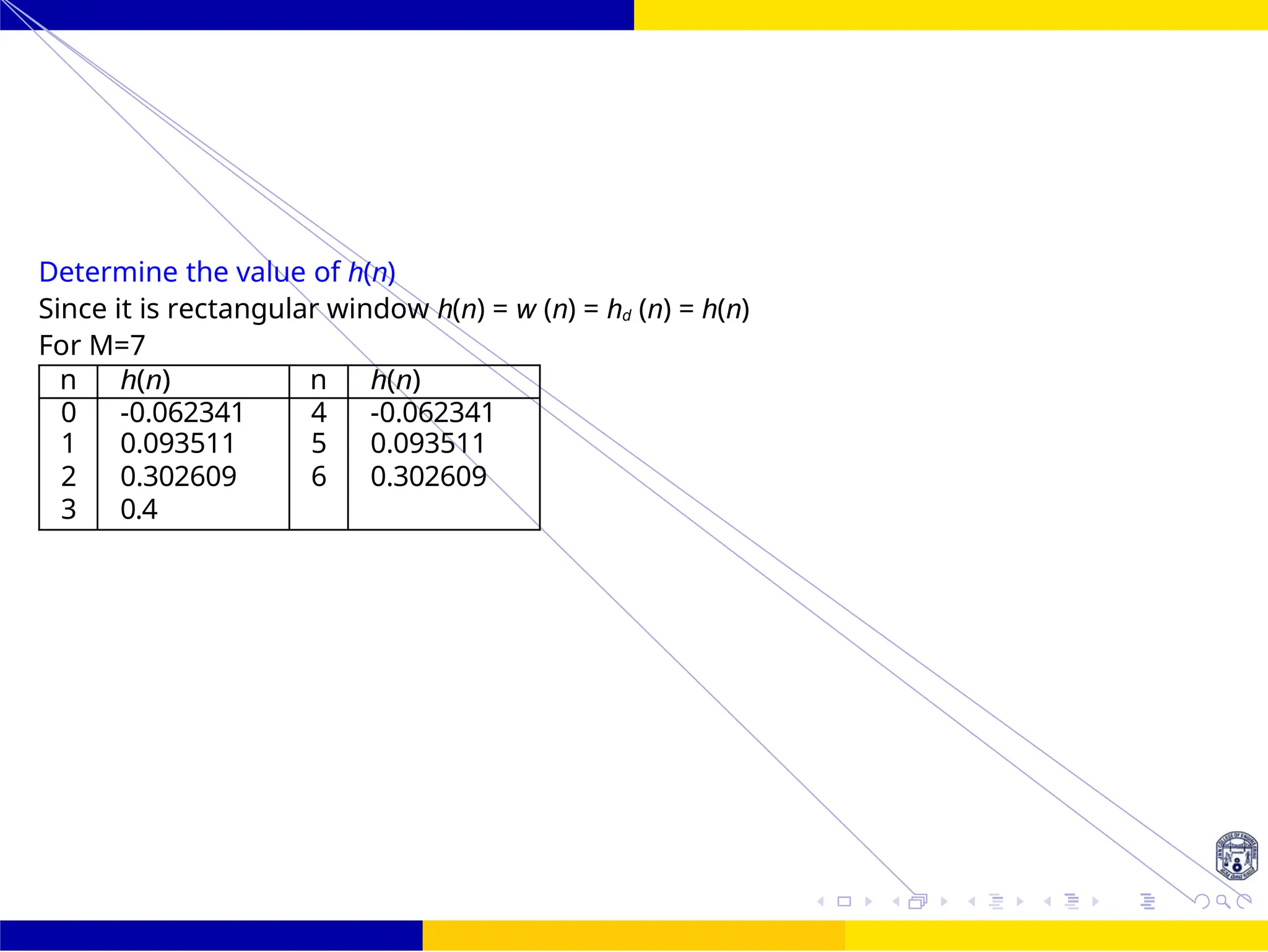
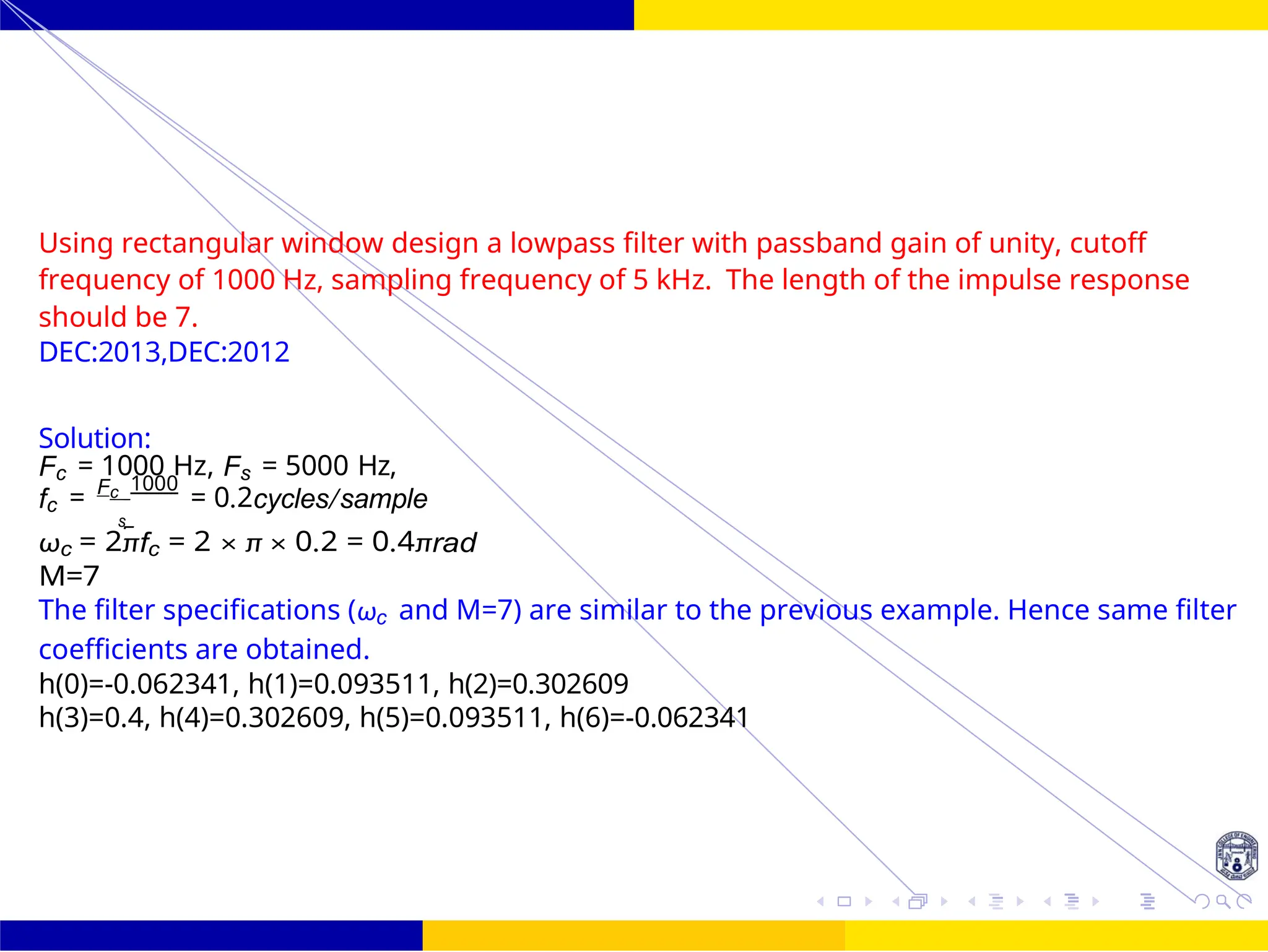
![∫
∫
FIR Filter Design Low Pass FIR Filter
Design
72 /
October 25,
UNIT - 7: FIR Filter
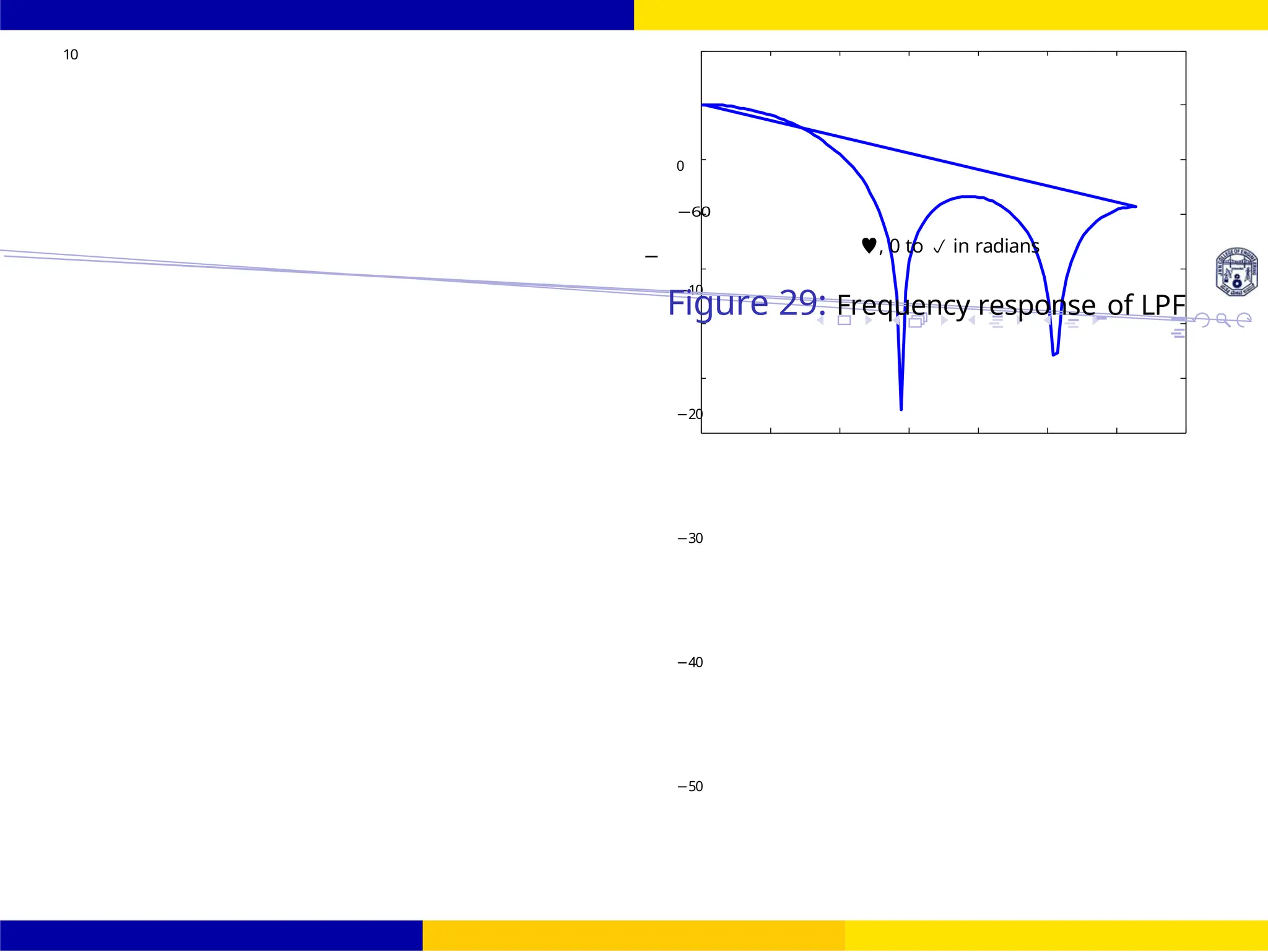
Dr. Manjunatha. P (JNNCE)
1
H (e j )
d
Design a normalized linear phase FIR low pass filter having phase delay of τ = 4 and at
least 40 dB attenuation in the stopband. Also obtain the magnitude/frequency response
of the filter.
Solution: The linear phase FIR filter is nor-
malized means its cut-off frequency is of ωc =
1rad/sample
The length of the filter with given τ is related by
M — 1
τ = 1 0 1
2
For τ = 4 M=9
Desired unit sample response hd (n)
is
Figure 28: Frequency response
of LPF
hd (n) =
1 ωc
2π
−ωc
e−jωτ
ejωn
dω
when n /=
4 sin[(n — 4)]
1 1
=](https://image.slidesharecdn.com/dspmodule4ppt-241209183808-f5b6e07b/75/dsp-module-4-pptpptrpppptxppppppppp-docx-88-2048.jpg)
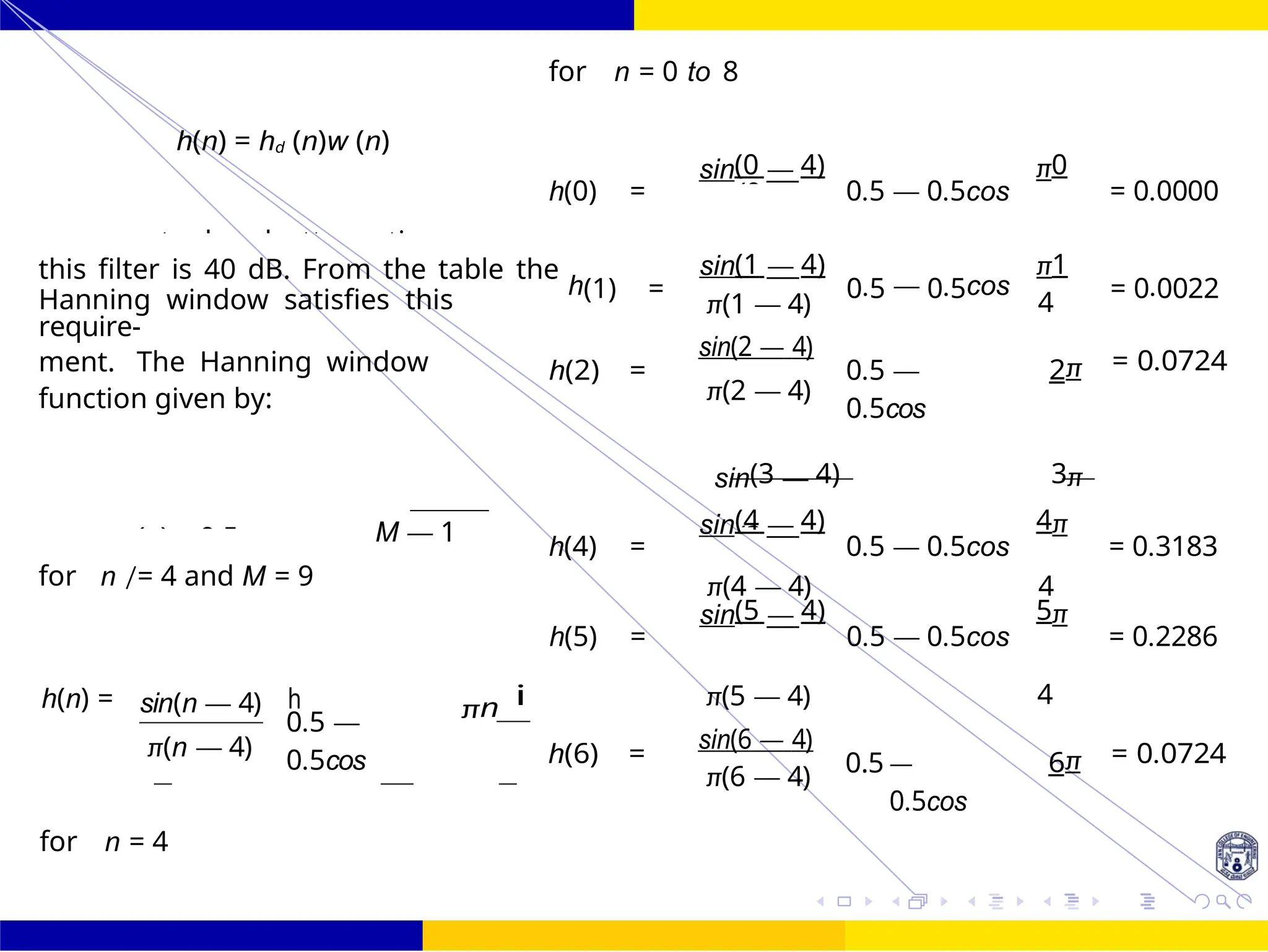

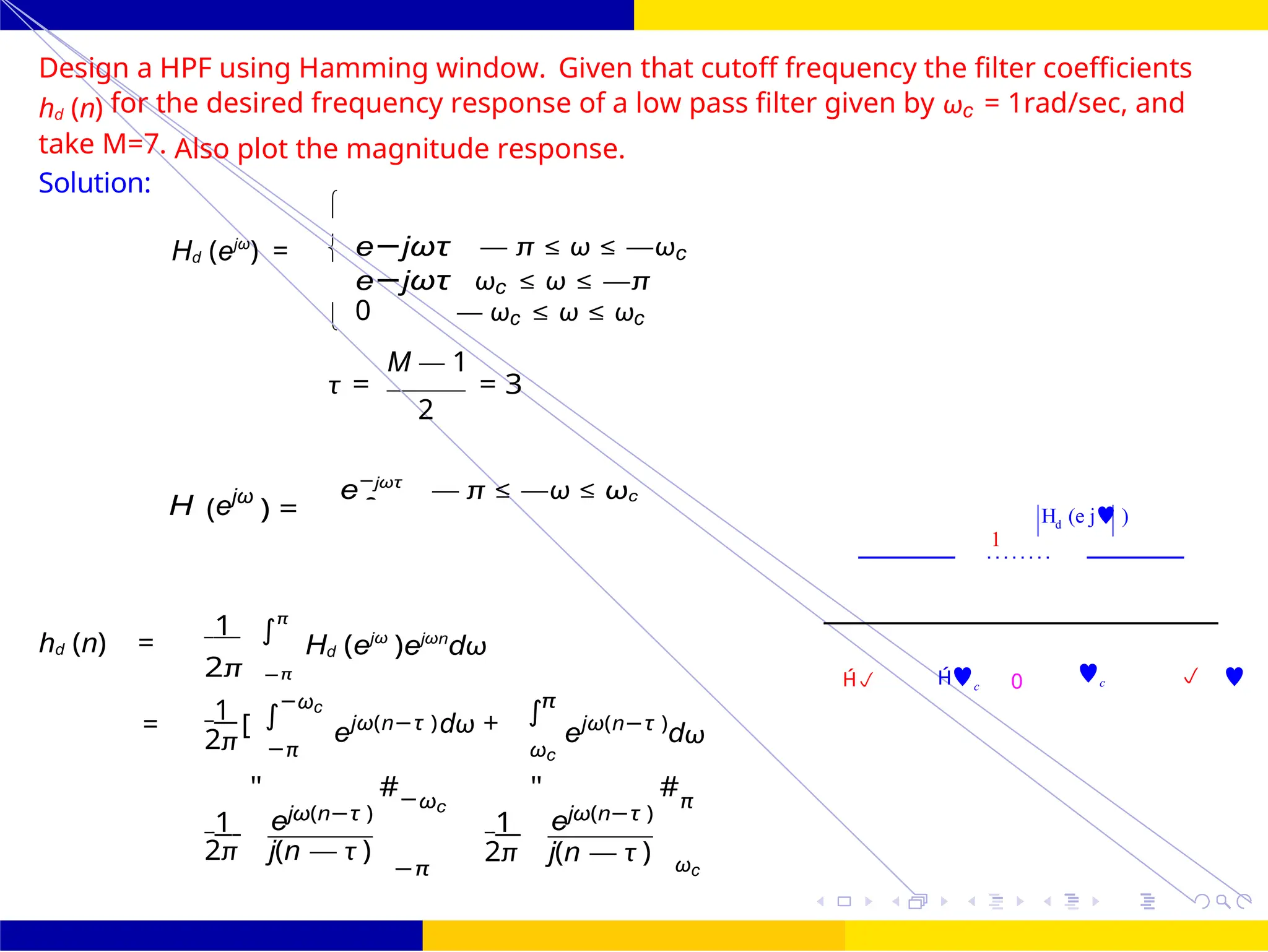
![π
d
π (n — (n — π
c
π
π(n — M
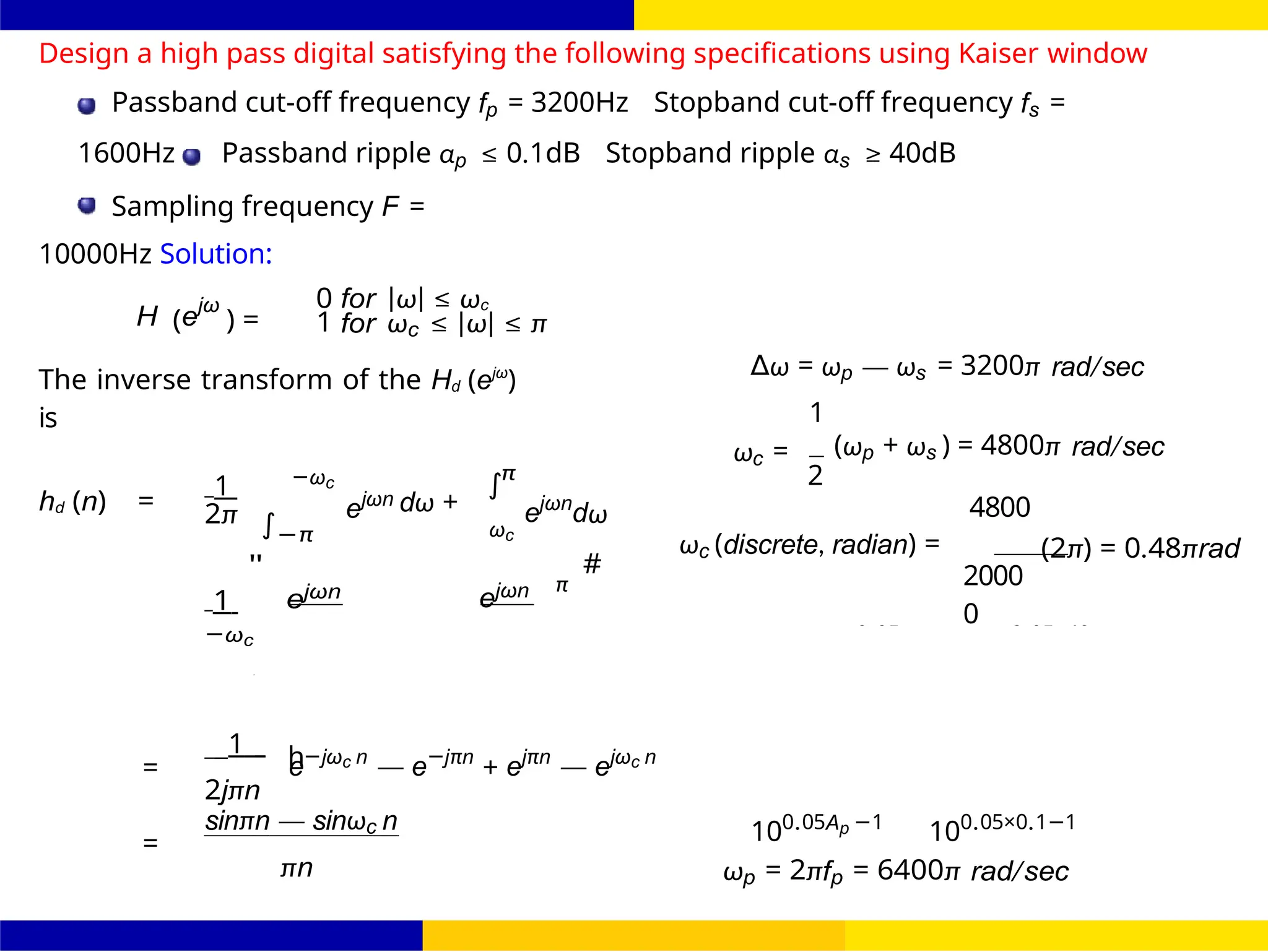
FIR Filter Design High Pass FIR Filter
Design
80 /
October 25,
UNIT - 7: FIR Filter
Dr. Manjunatha. P (JNNCE)
hd (n) =
1
"
ejπ(n−τ )
— e−jπ(n−τ )
— ejωc (n−τ )
— e−jωc (n−τ )
#
π(n — τ )
1
=
π(n — τ )
2j
[sinπ(n — τ ) — sinωc (n — τ ]
τ = 3 ωc = 1 hd (n) = 1
[sinπ(n — 3) — sin(n — 3)] when
n = τ using L Hospital rule
h (n) =
1 sinπ(n — 3)
—
sinωc (n — 3)
=
1
[π — ω ] =
1
[π — 1]
The given window function is Hamming window. In this case h(n) = hd (n)ω(n)) for 0 ≤ n ≤ 6
w (n) = 0.54 — 0.46cos
2πn
M — 1
h(n) =
1
[sinπ(n — 3) — sin(n — 3)] × 0.54 — 0.46cos
2πn
n h(n) n h(n)
0 -0.00119 4 -0.00119](https://image.slidesharecdn.com/dspmodule4ppt-241209183808-f5b6e07b/75/dsp-module-4-pptpptrpppptxppppppppp-docx-96-2048.jpg)
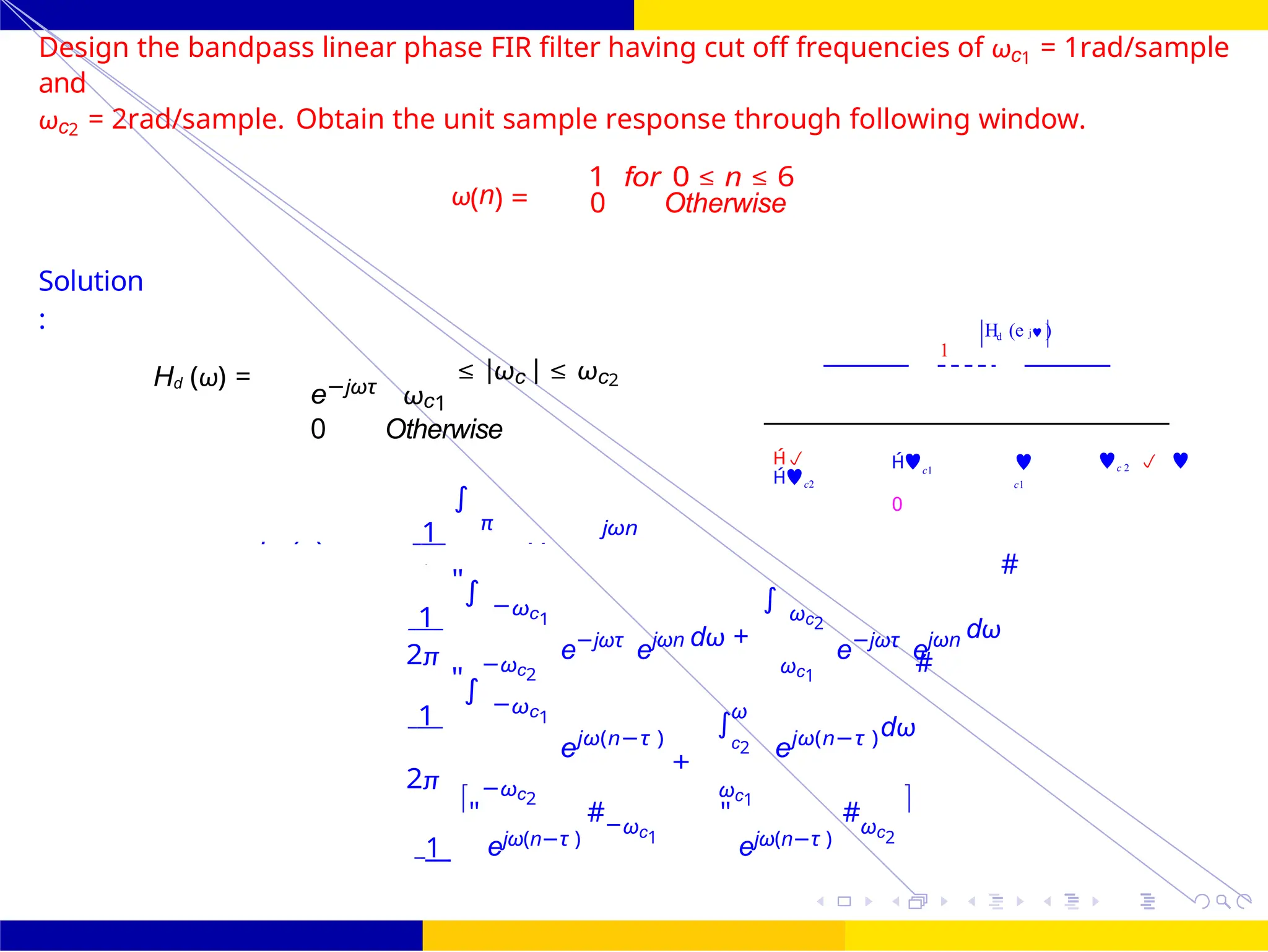

![FIR Filter Design Band Pass FIR Filter
Design
October 25, 93 /
UNIT - 7: FIR Filter
Dr. Manjunatha. P (JNNCE)
2π j(n — τ )
1
−ωc2
2π j(n — τ )
ωc2
=
π(n — τ )
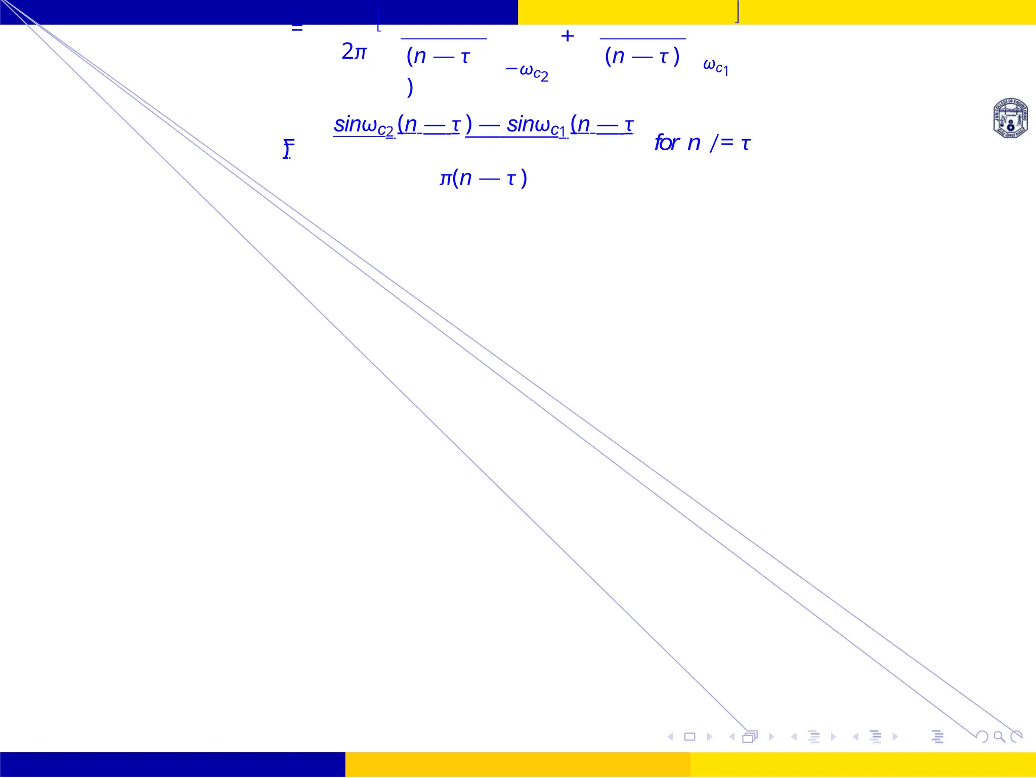
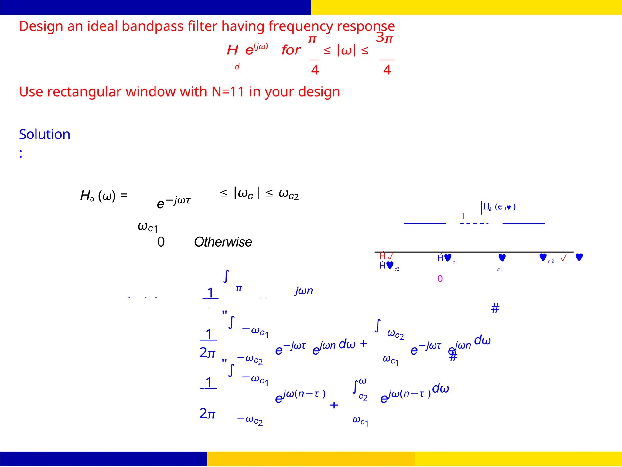
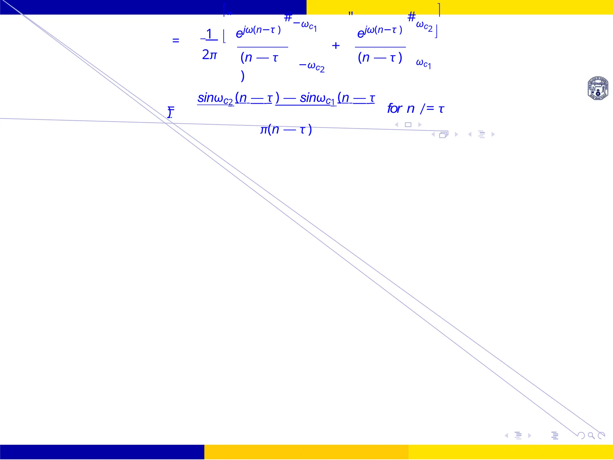
[sinωc2(n — τ ) — sinωc1(n — τ ]](https://image.slidesharecdn.com/dspmodule4ppt-241209183808-f5b6e07b/75/dsp-module-4-pptpptrpppptxppppppppp-docx-109-2048.jpg)
![d
FIR Filter Design Band Pass FIR Filter
Design
94 /
October 25,
UNIT - 7: FIR Filter
Dr. Manjunatha. P (JNNCE)
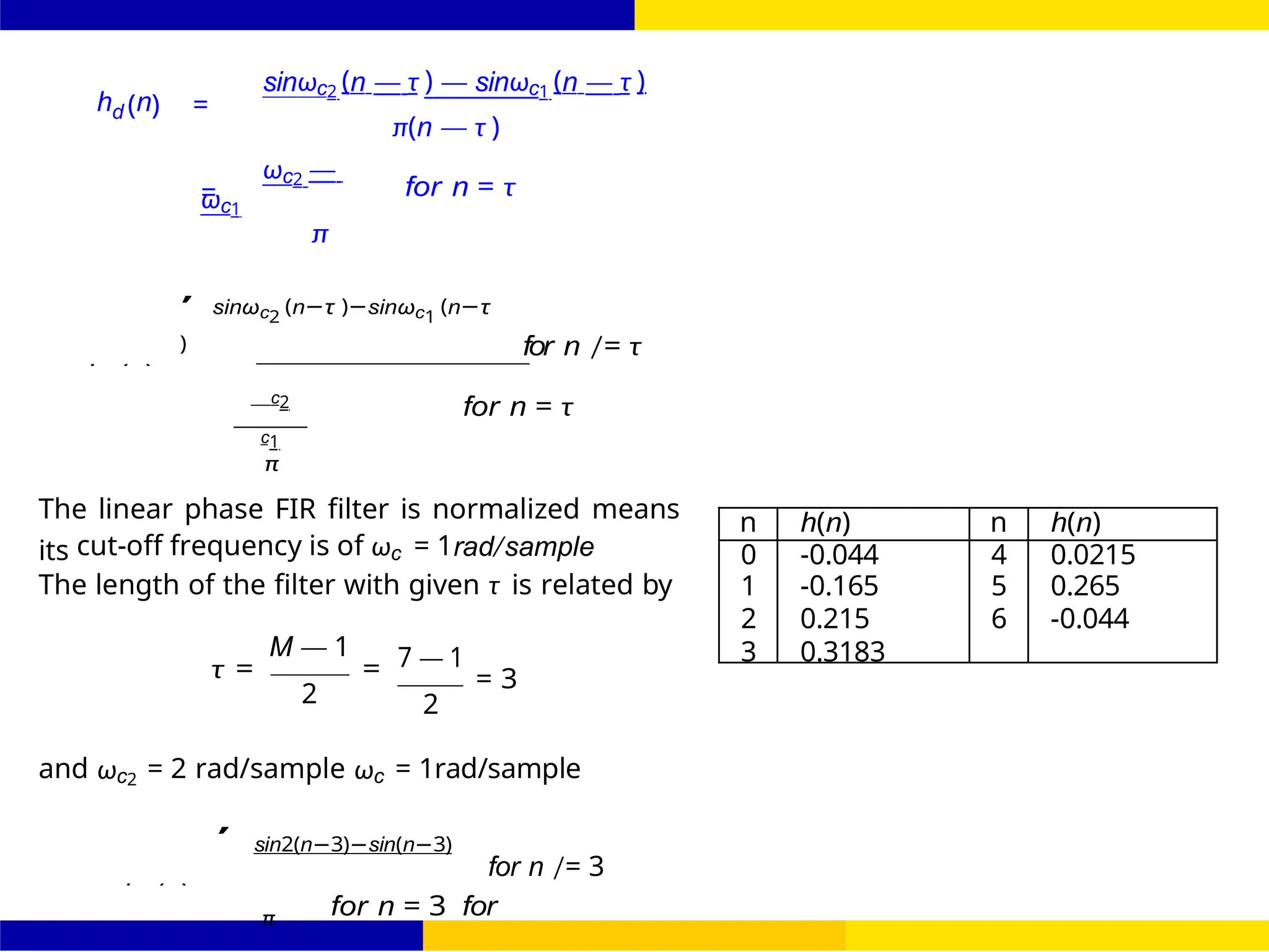
τ =
M−1
=
7−1
= 3
2 2
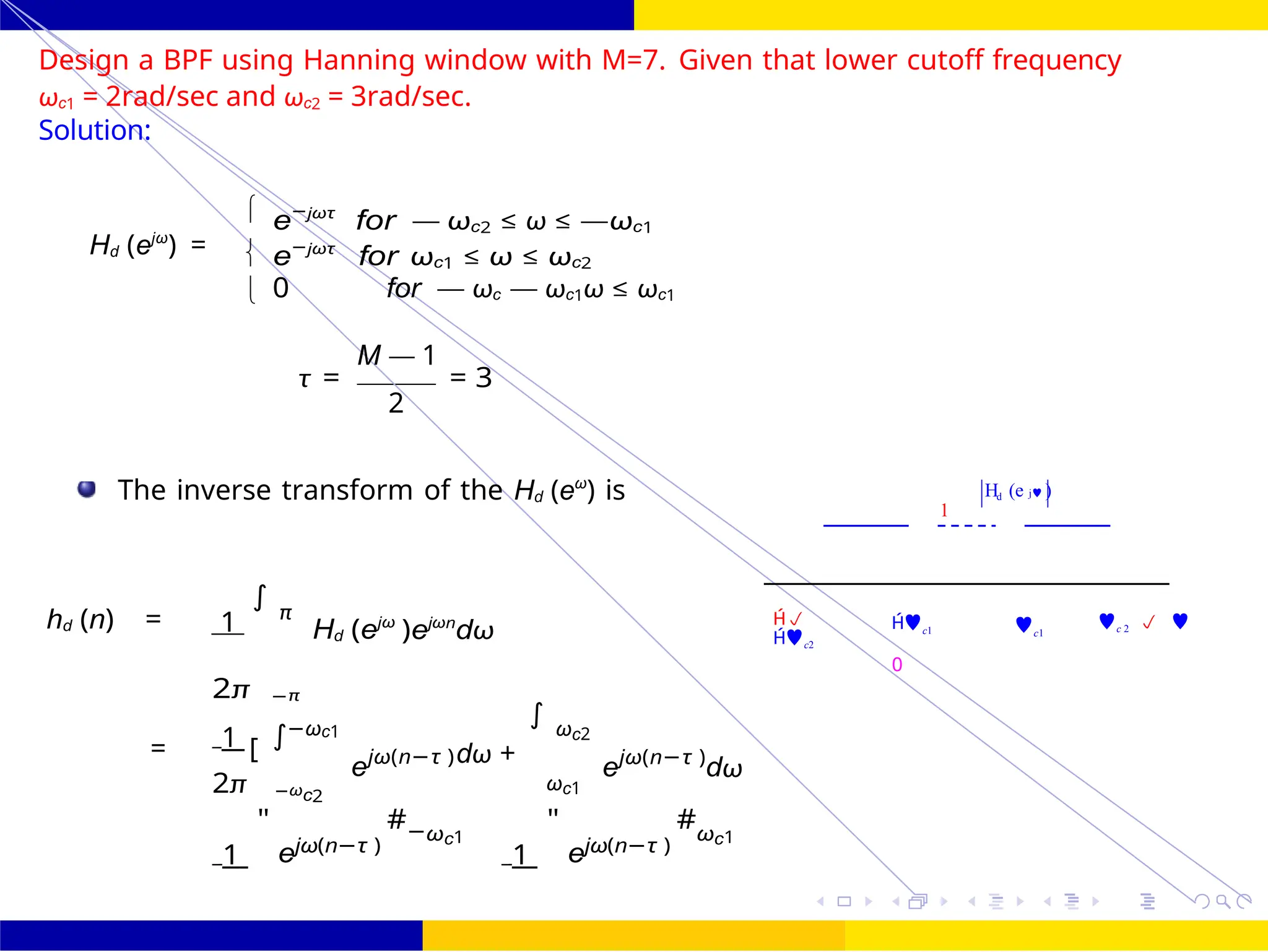
ωc1 = 2 rad/sec ωc2 = 3 rad/sec
for n /= 3
hd (n) = 1
π(n — 3)
[sin3(n — 3) — sin2(n — 3)]
for n = τ
h (n) =
1
lim
sinωc2(n — τ )
— lim
sinωc1(n — τ )
hd (n) = 1 1
[ωc2 — ωc1] =
π π
The given window function is Hanning window
ω(n) = 0.5 — 0.5cos 2πn
M —
1
π n (n — n (n —
n h(n) n h(n)
0 0 4 0
1 0.0189 5 0.0189
2 -0.01834 6 -0.01834
3 0.3183](https://image.slidesharecdn.com/dspmodule4ppt-241209183808-f5b6e07b/75/dsp-module-4-pptpptrpppptxppppppppp-docx-110-2048.jpg)
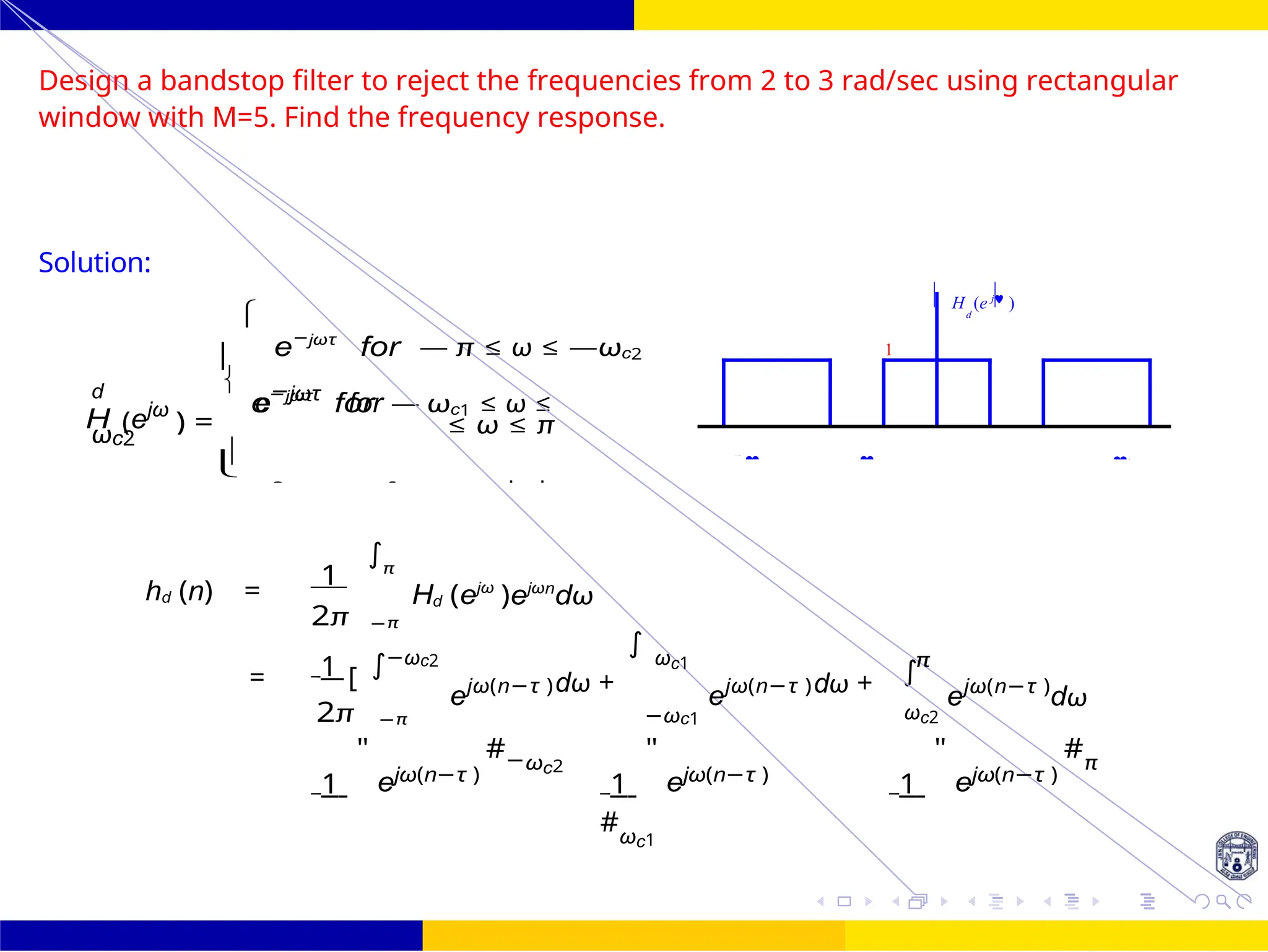
![FIR Filter Design Bandstop FIR Filter
Design
October 25, 99 /
UNIT - 7: FIR Filter
Dr. Manjunatha. P (JNNCE)
2π j(n — τ )
−π
1
2π j(n — τ )
−ωc1
2π j(n — τ )
ωc2
=
π(n — τ )
[sinωc1(n — τ ) + sinπ(n — τ — sinωc2(n — τ ]
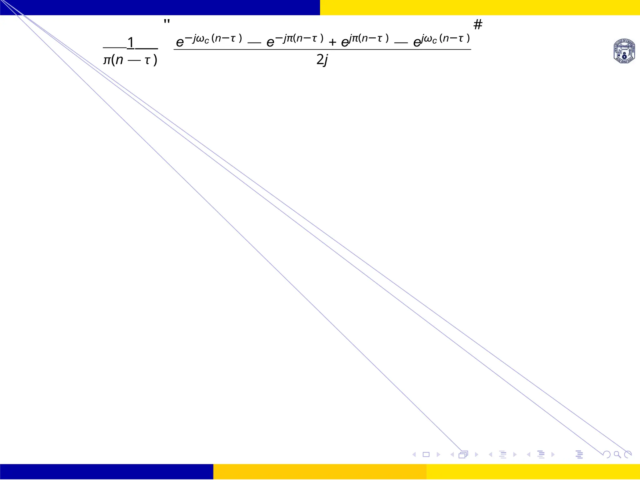
+](https://image.slidesharecdn.com/dspmodule4ppt-241209183808-f5b6e07b/75/dsp-module-4-pptpptrpppptxppppppppp-docx-115-2048.jpg)
![d
FIR Filter Design Bandstop FIR Filter
Design
100 /
October 25,
UNIT - 7: FIR Filter
Dr. Manjunatha. P (JNNCE)
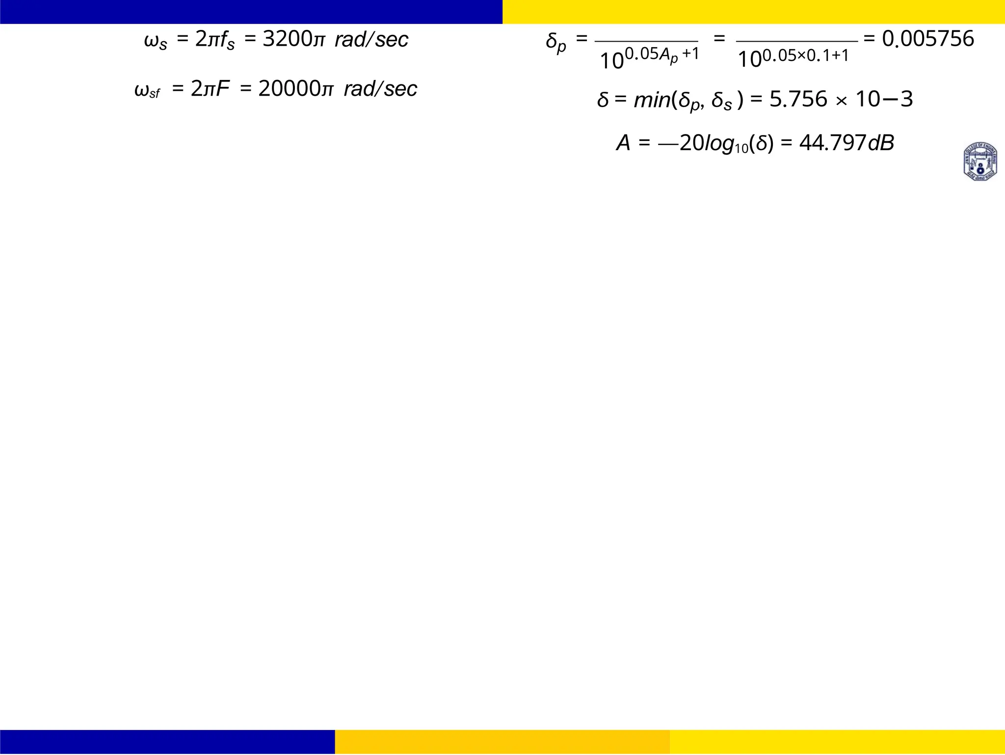
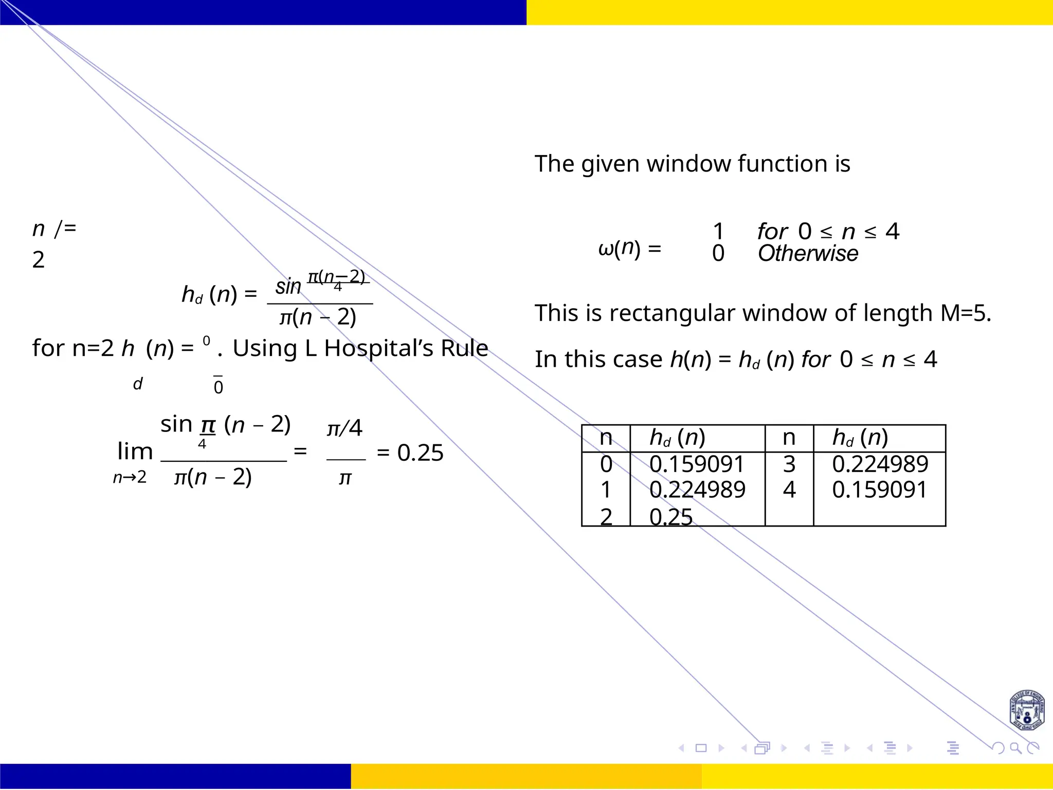
The inverse transform of the Hd (eω
) is
τ = M−1
= 5−1
= 2 ωc1 = 2 rad/sec ωc2 = 3 rad/sec
2 2
hd (n) = 1
π(n — 2)
[sin2(n — 2) + sinπ(n — 2) — sin3(n — 2)] for n /= 2
for n =
τ
h (n) =
1
lim
sinωc1(n — τ )
+ lim
sinπ(n — τ )
— lim
sinωc2(n — τ )
hd (n) = 1
[ωc1 + π — ωc2] =
π
1
[π — 1]
π
The given window function is Rectangular window
ω(n) = 1 0 ≤ n ≤ M — 1
This is rectangular window of length M=5.
In this case h(n) = hd (n)ω(n) = hd (n) for 0 ≤ n ≤ 4
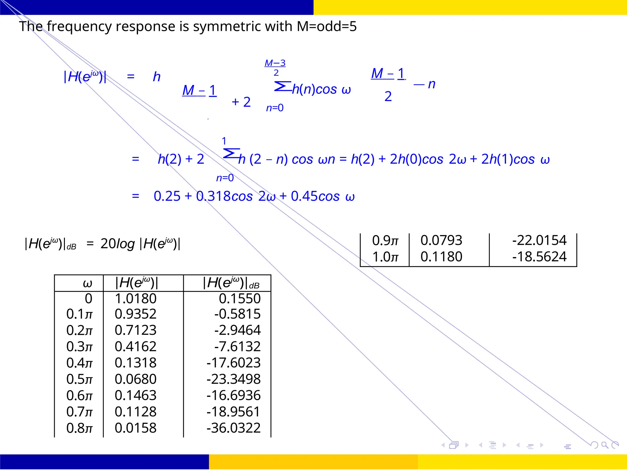
π n (n — n (n — n (n —](https://image.slidesharecdn.com/dspmodule4ppt-241209183808-f5b6e07b/75/dsp-module-4-pptpptrpppptxppppppppp-docx-116-2048.jpg)
![FIR Filter Design Bandstop FIR Filter
Design
101 /
October 25,
UNIT - 7: FIR Filter
Dr. Manjunatha. P (JNNCE)
1
hd (n) =
π(n — 2)
[sin2(n — 2) + sinπ(n — 2) — sin3(n — 2)] for n /= 2](https://image.slidesharecdn.com/dspmodule4ppt-241209183808-f5b6e07b/75/dsp-module-4-pptpptrpppptxppppppppp-docx-117-2048.jpg)
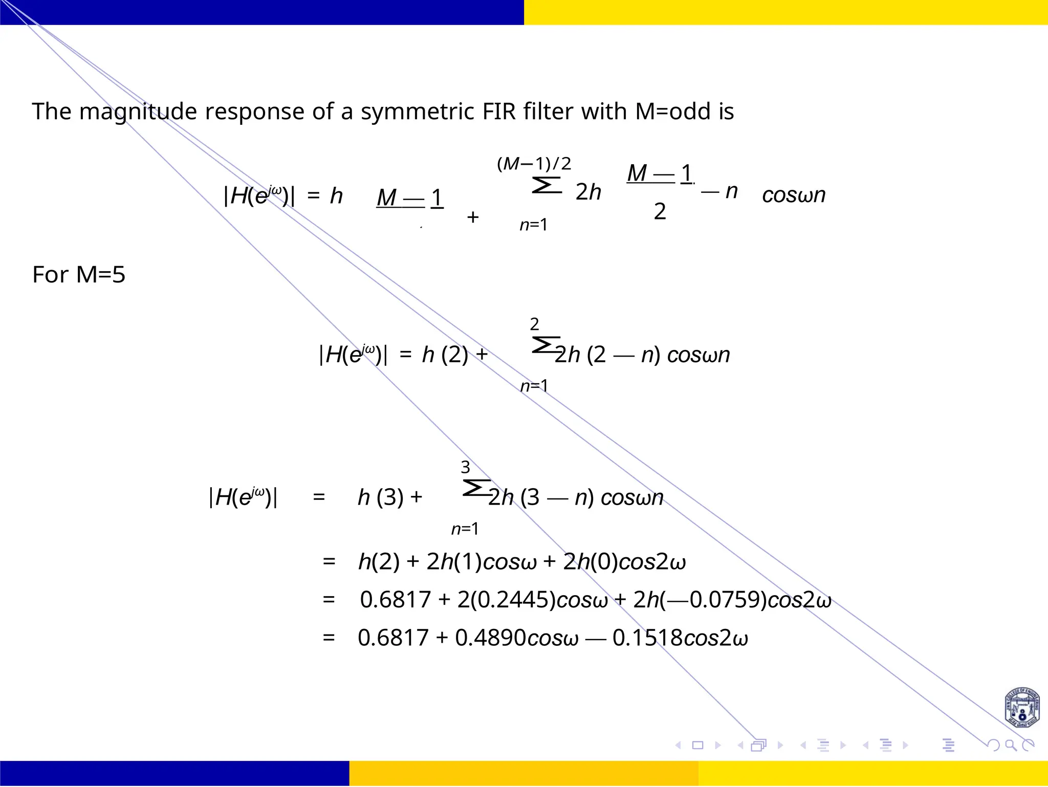
![FIR Filter Design Bandstop FIR Filter
Design
102 /
October 25,
UNIT - 7: FIR Filter
Dr. Manjunatha. P (JNNCE)
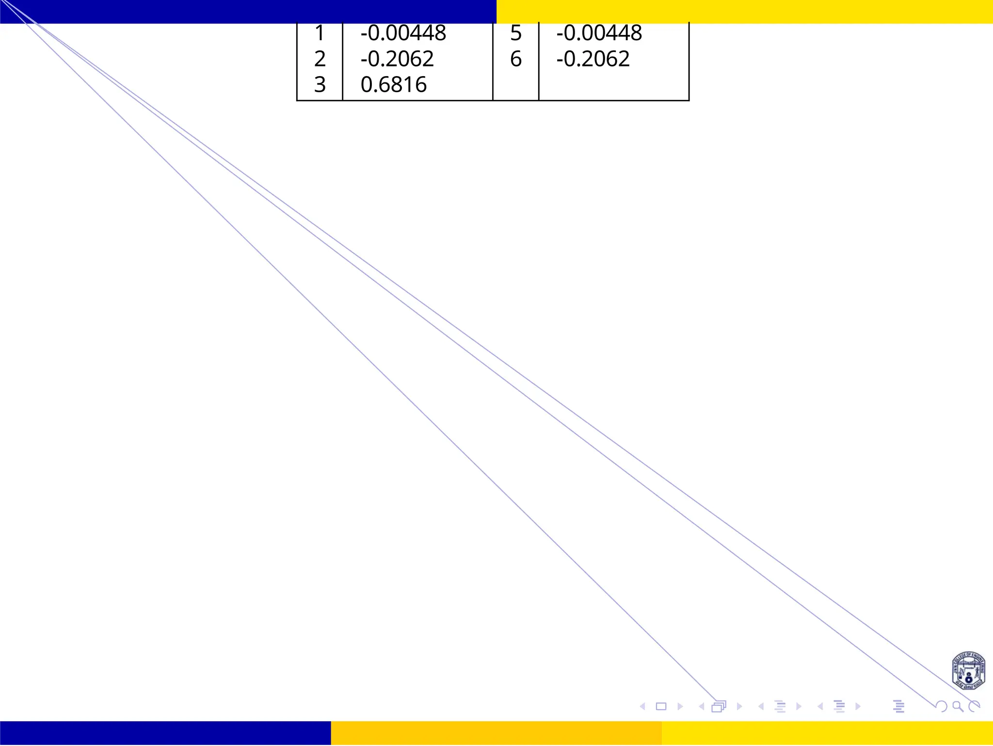
n = 0 h(0) =
sin2(0 — 2) + sinπ(0 — 2) — sin3(0 — 2)
= —0.0759
π(0 — 2)
n = 1 h(1) =
sin2(1 — 2) + sinπ(1 — 2) — sin3(1 — 2)
= 0.2445
π(1 — 2)
n = 2 h(2) = 1
[π — 1] = 0.6817
π
n = 3 h(3) =
sin2(3 — 2) + sinπ(3 — 2) — sin3(3 — 2)
= 0.2445
π(3 — 2)
n = 4 h(4) =
sin2(4 — 2) + sinπ(4 — 2) — sin3(4 — 2)
= —0.0759
π(4 — 2)
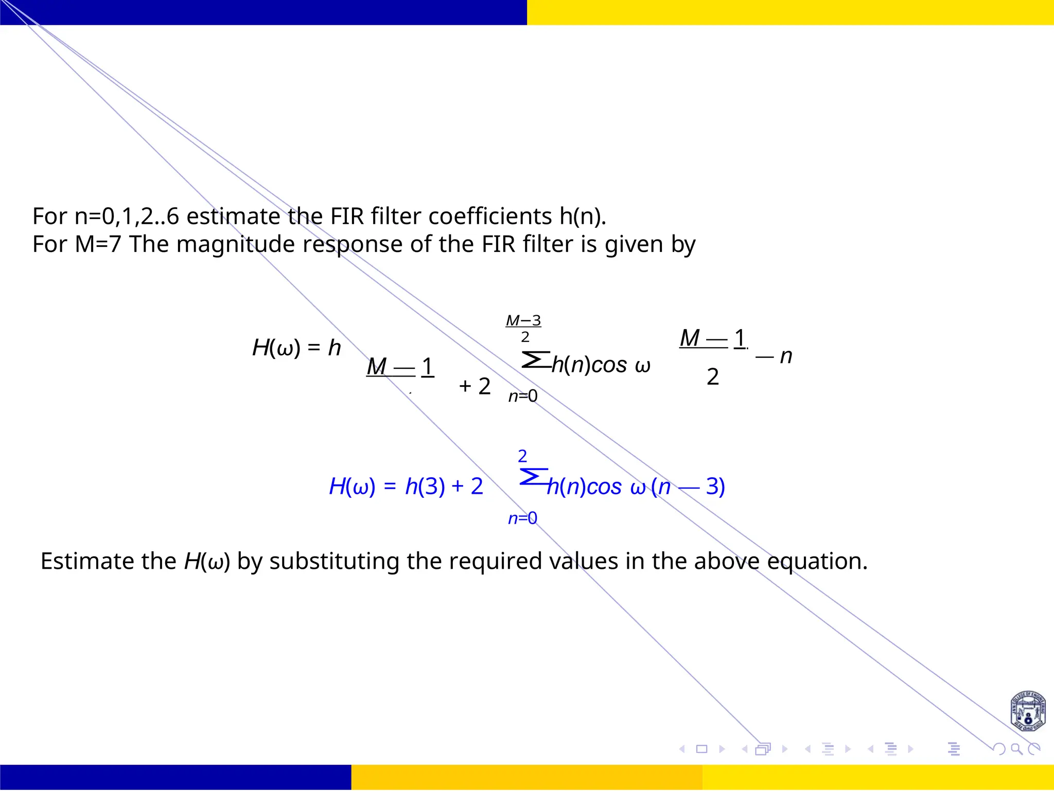
M−1 4
H(z ) =
Σ
h(n)z −n
=
Σ
h(n)z −n
= h(0) + h(1)z −1
+ h(2)z −2
+ h(3)z −3
+ h(4)z −4
n n](https://image.slidesharecdn.com/dspmodule4ppt-241209183808-f5b6e07b/75/dsp-module-4-pptpptrpppptxppppppppp-docx-118-2048.jpg)

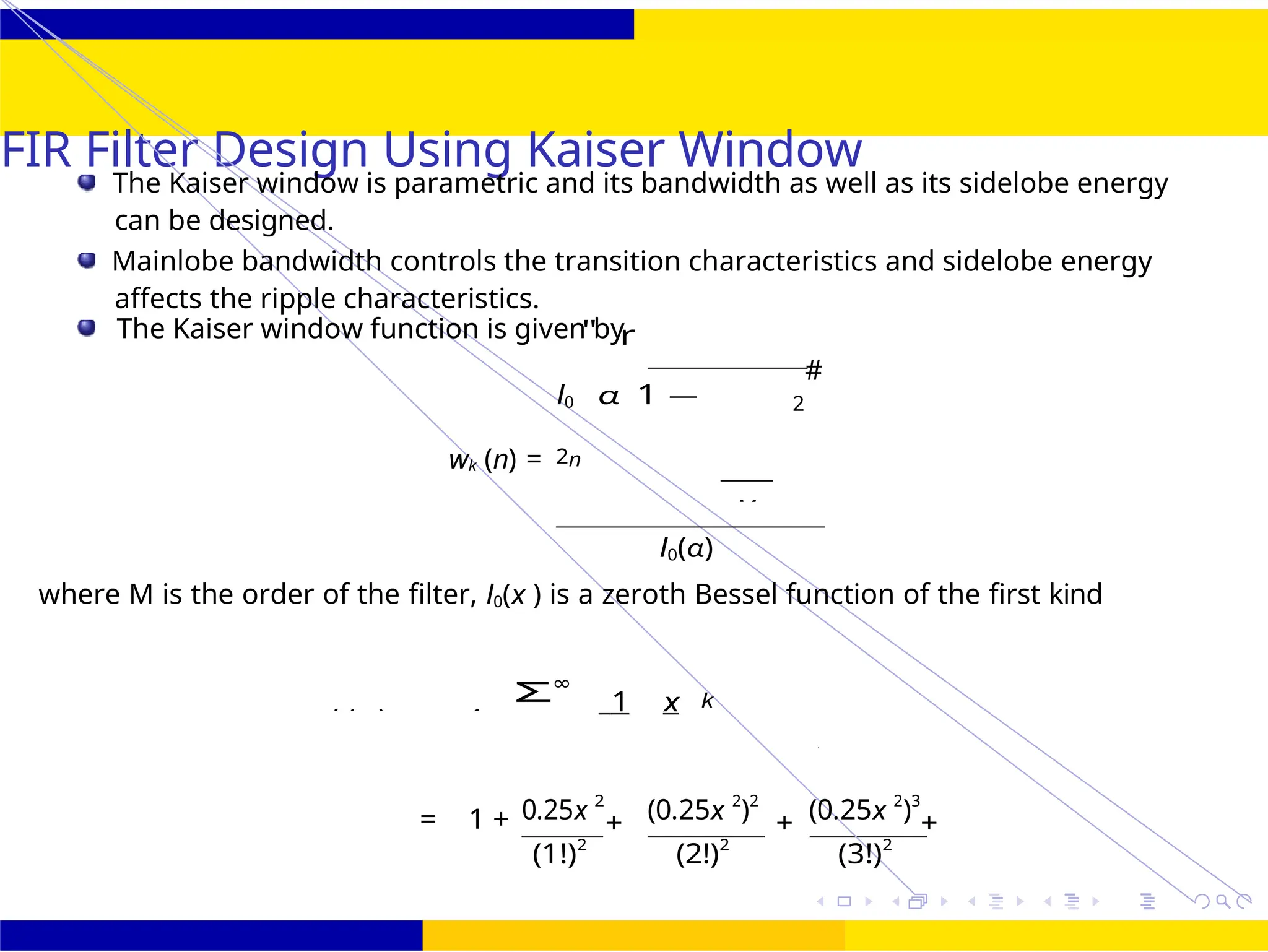
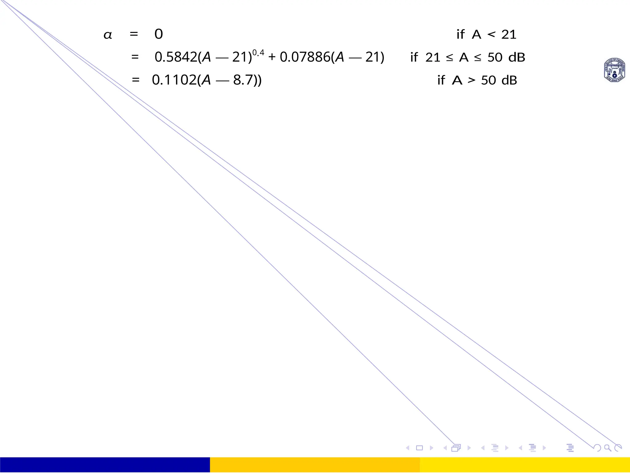
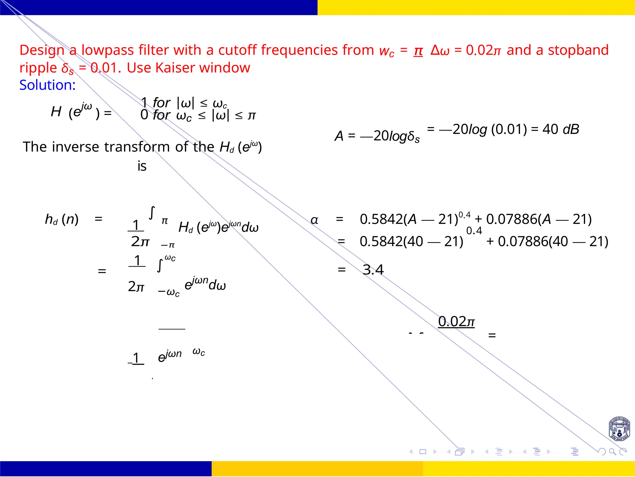
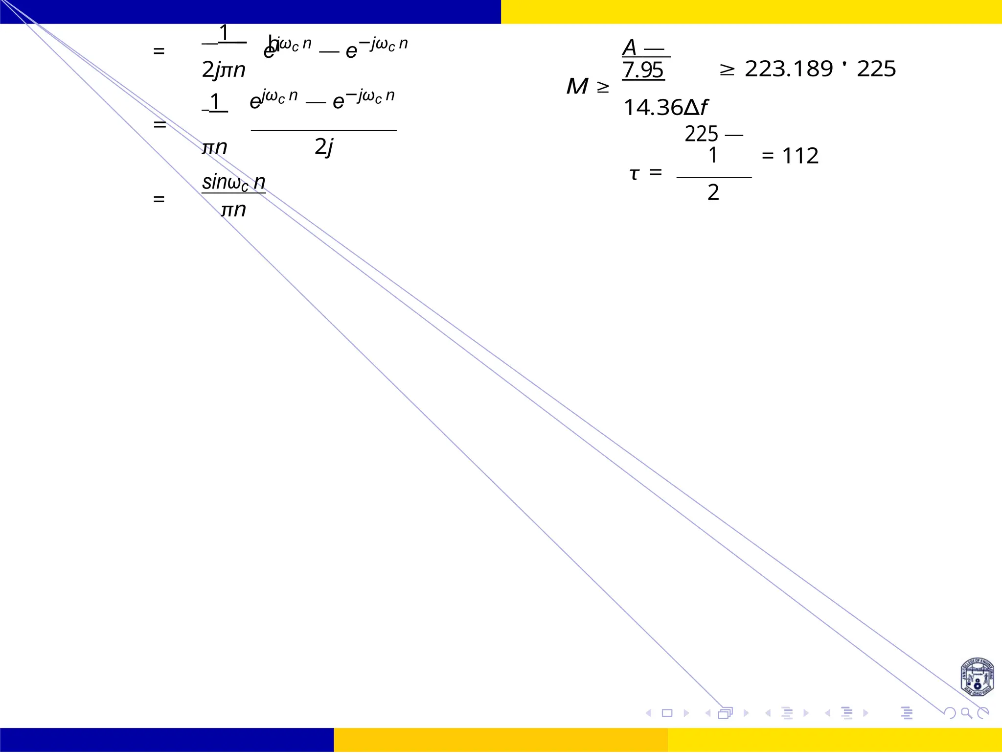
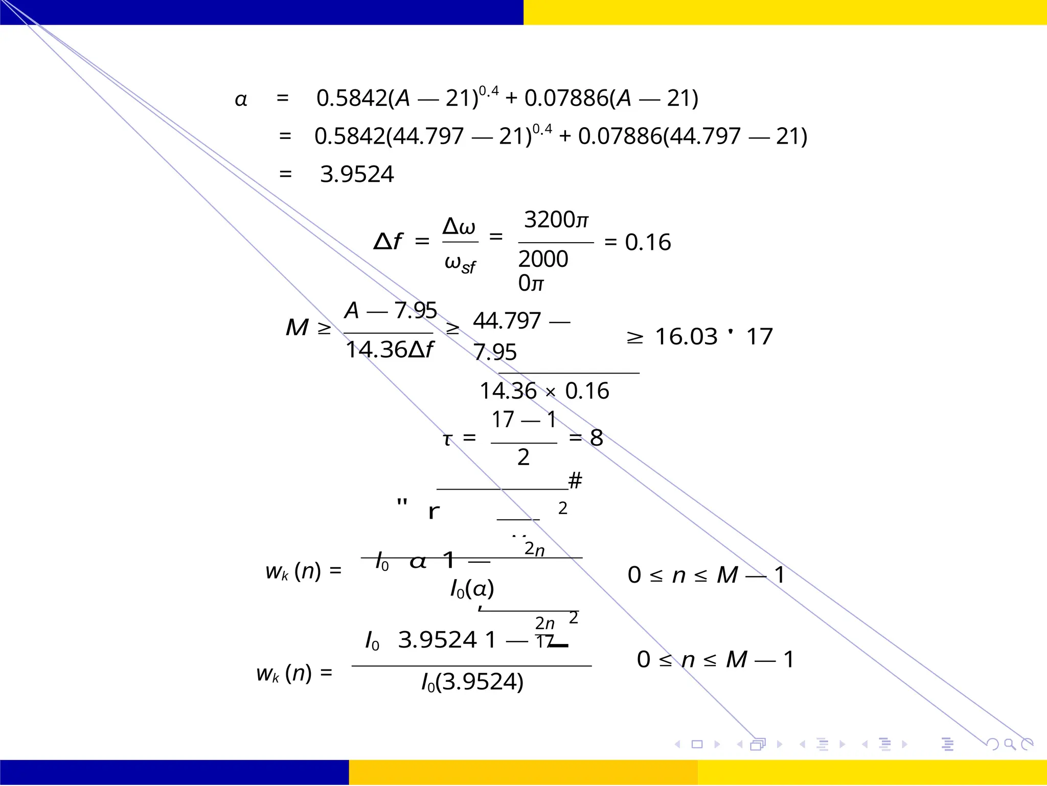
![M
I0 3.4
,
1 —
FIR Filter Design FIR Filter Design Using Kaiser
Window
114 /
October 25,
UNIT - 7: FIR Filter
Dr. Manjunatha. P (JNNCE)
2
#
I0
"
α
r
1 —
2n
wk (n) =
wk (n) =
0 ≤ n ≤ M — 1
I0(α)
2n 2
224
0 ≤ n ≤ M — 1
I0(3.4)
I0 3.4
,
1 —
2n 2
wher
e
h(n) = hd × wk (n) =
1
[sinωc n] ×
πn I0(3.4)
224
'
ωc = ωc +
∆ω
= 0.25π +
2
0.02π
= 0.26π
2](https://image.slidesharecdn.com/dspmodule4ppt-241209183808-f5b6e07b/75/dsp-module-4-pptpptrpppptxppppppppp-docx-130-2048.jpg)
![I0 5.48
,
1 —
FIR Filter Design FIR Filter Design Using Kaiser
Window
Dr. Manjunatha. P (JNNCE) UNIT - 7: FIR Filter October 25, 118 /
1 ejωc n — e−jωc n
= 0.24π + 0.1π
= 0.29π
2
πn 2j
=
sinωc n
πn
h(n) = hd × wk (n) =
1
π(n — τ )
[sinωc (n — τ )] ×
2n 2
224
I0(5.5)
=](https://image.slidesharecdn.com/dspmodule4ppt-241209183808-f5b6e07b/75/dsp-module-4-pptpptrpppptxppppppppp-docx-134-2048.jpg)
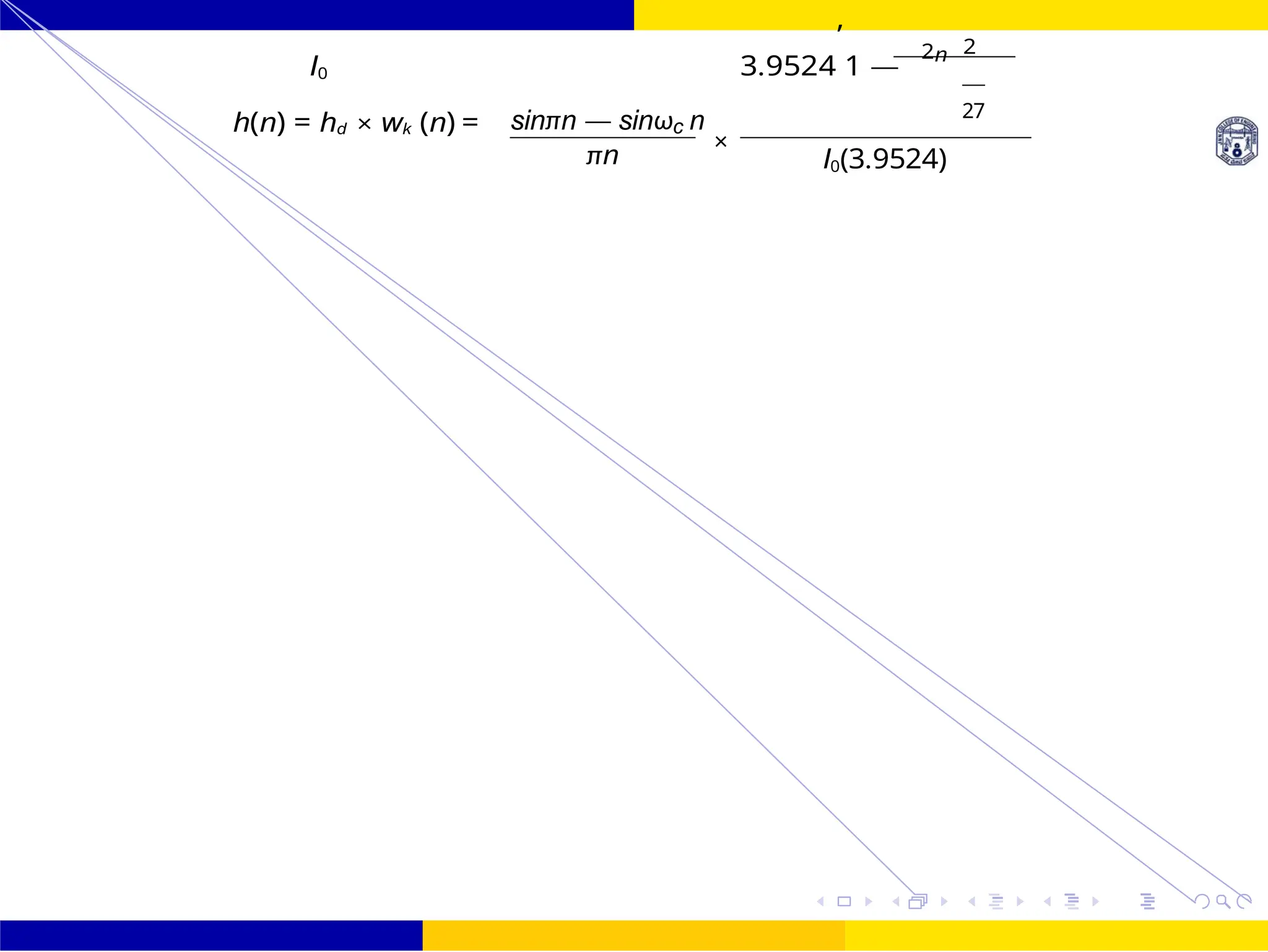
![FIR Filter Design FIR Filter Design Using Kaiser
Window
122 /
October 25,
UNIT - 7: FIR Filter
Dr. Manjunatha. P (JNNCE)
I0 3.9524
,
1 —
2n 2
h(n) = hd × wk (n) = 1
[sinωc n] ×
πn
27
I0(3.9524)](https://image.slidesharecdn.com/dspmodule4ppt-241209183808-f5b6e07b/75/dsp-module-4-pptpptrpppptxppppppppp-docx-138-2048.jpg)