This document is a thesis on Brownian motion and stochastic calculus. It contains an introduction that defines random walks, Brownian motion, and establishes Brownian motion as the limit of a random walk as the number of steps increases. The thesis will explore properties of random walks and Brownian motion through simulations and theoretical analysis. It will also provide an introduction to stochastic calculus and its applications in finance, such as the Black-Scholes option pricing formula.

![CHAPTER 1. INTRODUCTION 3
where x is the floor function, that is, it takes the largest integer that is smaller or equal than
x. Notice that a random walk is defined for discrete values. The previous definition admits any
value t ≥ 0. Because we have S nt instead of S t for big enough n the term
1
√
n
S nt will
change quickly as t grows. In a way we have made a ‘continuous’ random walk.
Theorem 1.0.3. With {Xn
} defined by (1.8), we have that for any t > 0
Xn
t
d
−→ Bt as n → ∞ (1.9)
where {Bt, t ≥ 0} is a Brownian motion.
Proof. First we see that ψn,t
P
−→ 0 as n → ∞. We have that
|ψn,t| = Xn
t −
1
√
n
S nt ≤
1
√
n
|ξ nt +1| (1.10)
and by Chebyshev inequality
P (|ψn,t| > ε) ≤ P
1
√
n
|ξ nt +1| > ε ≤
E 1√
n
ξ nt +1
2
ε2
=
1
ε2n
→ 0 (1.11)
Because ψn,t
P
−→ 0 this also means that ψn,t
d
−→ 0 se we can use Slutsky’s theorem (1.0.1) and
we obtain Xn
t has the same limit as
1
√
n
S nt .
By the Central Limit Theorem and because nt /n → t
1
nt
S nt
d
−→ N, N ∼ N(0, 1) (1.12)
If we consider Yn =
nt
√
n
, then Y
d
−→
√
t = c and we can use Slutzky’s theorem to
1
nt
S nt · Yn:
1
√
n
S nt =
1
√
n
nt
nt
S nt =
1
nt
S nt · Yn
d
−→
√
tN (1.13)
and because Xn
t has the same limit as
1
√
n
S nt we have that
Xn
t
d
−→
√
tN
d
= Bt (1.14)
This result gives us a feeling on the concept of Brownian motion, as we can understand it as a
limit of a random walk.
We have assumed that the random variables ξi can only take discrete values 1 and −1. There
is a stronger result, in which we don’t need to assume that the random variables take only
these two discrete values. It is called Donsker’s invariance Theorem and it is a generalization
of what we have just seen. If we take i.i.d random variables ξi Theorem (1.0.3) still holds true.
We won’t show this result here, but more details can be found in the book of Billinsgley [2].
The following Proposition can translate some properties we see in random walks to properties
in Brownian motion.](https://image.slidesharecdn.com/edc87572-6bc2-40ac-a67c-f53bfedb3e6d-160930223103/85/tfg-8-320.jpg)
![CHAPTER 1. INTRODUCTION 4
Proposition 1.0.1. Let C([0, ∞)) be the space of continuous functions with the topology of
uniform convergence on compacts. Then for every continuous Ψ : C([0, ∞]) → R we have that
Ψ(Xn
)
d
−→ Ψ(B) (1.15)
where Xn is defined by (1.8) and B = (Bt, t ≥ 0) is the Brownian motion.
Example 1.0.1. Let’s consider Y n
= max
0≤t≤T
Xn
t . The functional Ψ(f) = max
0≤t≤T
f(t) is continu-
ous, so we can apply Proposition (1.0.1). It tells us that
Y n d
−→ max
0≤t≤T
Bt (1.16)
This tool sometimes can be of great help, because if one has proved some property for the
random walk this Proposition can help with the proof for the Brownian motion taking limits.
However, we will encounter non-continuous functionals such as the stopping time:
τ = inf{n > 0, Sn = a} (1.17)
Because this functional is not continuous we cannot apply theorem (1.0.1). A consequence
of this is for example that to show the recurrence of the random walk and the recurrence
of Brownian motion we will need to prove these results separately. Although it seems quite
intuitive that properties in the random walk must keep true in the Brownian motion (and as a
matter of fact it almost always happens), we cannot deduce these results just taking limits.](https://image.slidesharecdn.com/edc87572-6bc2-40ac-a67c-f53bfedb3e6d-160930223103/85/tfg-9-320.jpg)
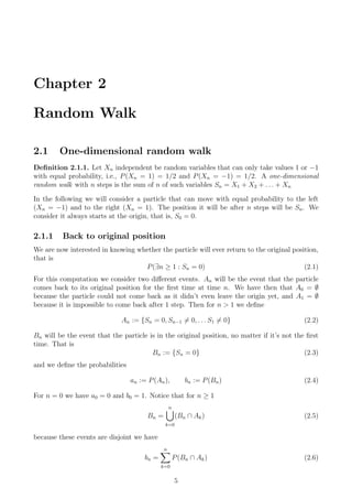
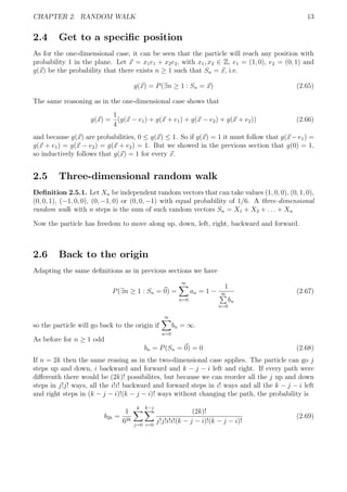
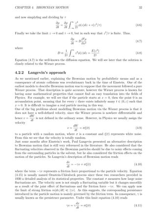
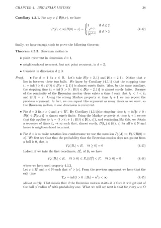
![CHAPTER 3. SIMULATIONS: RANDOM WALKS 17
values obtained by both the simulation and the theory.
N Theory Simulations Desviation (%)
2 25000 25030 0.1
4 6250 6196 -0.8
6 3125 3139 0.4
8 1953 1956 0.14
10 1367 1389 1.5
12 1025 1016 -0.9
14 806 780 -3.2
16 655 683 4.3
18 545 590 8.2
20 463 469 1.1
22 400 396 -1.1
24 350 359 2.5
26 310 293 -5.4
28 277 301 8.7
30 249 237 -4.8
N Theory Simulations Desviation (%)
32 226 240 6.3
34 206 235 14.1
36 189 176 -6.7
38 174 181 4.2
40 161 154 -4.2
42 149 149 0
44 139 128 -7.9
46 130 120 -7.6
48 122 96 -21.2
50 115 104 -9.2
52 108 115 6.5
54 102 104 2.0
56 96 91 -5.6
58 92 91 -0.5
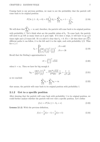
Table 3.1: This table gather both the theoretical and experimental frequencies, and also the
desviation with respect to the theoretical values.
The desviation has been calculated as
Desviation =
Experimental frequencies − Theoretical frequencies
Theoretical frequencies
· 100 (3.1)
Looking into the data in the table we observe a trend that we could not see in the plotted
graph. We observe that the desviation (i.e the error) grows as the number of steps grows. This
is something we should expect, because the number of particles that go back to origin after
N steps decreases as N grows. That means that we have less data available for N big and
therefore the simulations are less accurate. This is a direct implication of the Law of Large
Numbers (see page 8 of the reference [5]).
For the theoretical counts, we have used the formula 2.35. The expected count Y2m of the
number of particles that reach back the origin after 2m steps will be given by
E(Y2m) = N · a2m (3.2)
where N is the total number of simulations.
For example, the expected count of particles that come back to origin after 2 steps for 50000
simulations is
E(Y2m) = 50000 ·
1
2
= 25000 (3.3)
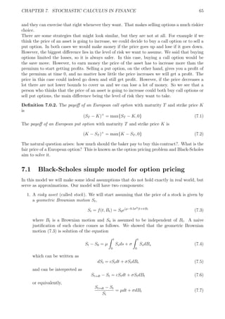
Now we will see another simulation in log-log scale.](https://image.slidesharecdn.com/edc87572-6bc2-40ac-a67c-f53bfedb3e6d-160930223103/85/tfg-22-320.jpg)
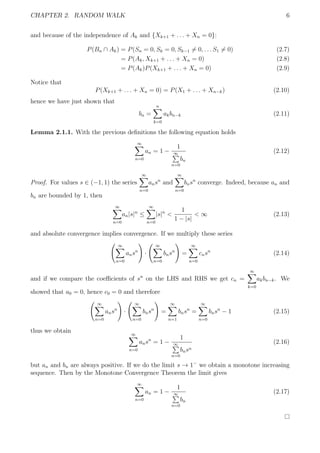
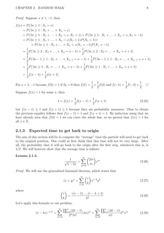
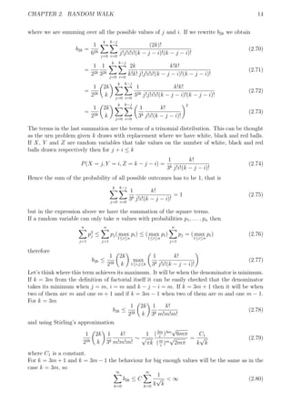
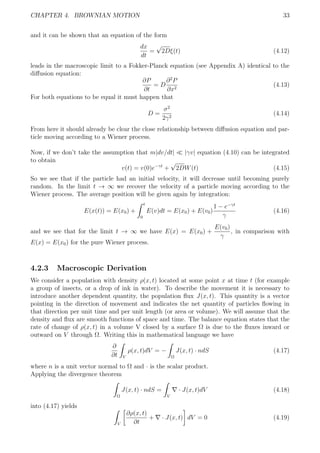
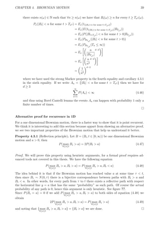
![CHAPTER 3. SIMULATIONS: RANDOM WALKS 18
Figure 3.2: Particles to reach back origin in log-log scale
It is important to remark that even though the bins in the figure (3.2) are the same width,
the more to the right they are the more number of steps they represent. To make it easier to
understand let’s take an example, the bin 0 to 1 is the sum of all the simulations in which the
particle returned back to the origin and took between e0
= 1 and e1
= 2.71 . . . steps. So we
now that the bin 0 to 1 only represent the case when the particle returned back to the origin
after 2 steps. If we take the bin 7 to 8 it represents all the simulations in which the particle
returned back to the origin and took between e7
= 1096.63 . . . and e8
= 2980.95 . . . steps. So
this bin counts for every simulation in which it took the particle 1098 steps, or 1100 steps,...,
or 2980 steps to go back to the origin.
We can collect this data in a table:
log(N) Theory Simulations Desviation
[0 − 1) 5000 4921 -1.5
[1 − 2) 1875 1906 1.6
[2 − 3) 1363 1356 -0.5
[3 − 4) 681 680 -0.1
[4 − 5) 426 445 4.4
[5 − 6) 257 285 10.8
[6 − 7) 156 146 -6.8
[7 − 8) 94 90 -5.1
3.1.1 Code
The following script runs M different simulations of random walks of length at most N. For
every simulation when the random walk reaches 0 for the first time it stops the simulation and
keeps the number of steps in a vector v.
def SimRandomWalk(N=100, M=1000):
v=[]
for l in range (1 ,M) :](https://image.slidesharecdn.com/edc87572-6bc2-40ac-a67c-f53bfedb3e6d-160930223103/85/tfg-23-320.jpg)
![CHAPTER 3. SIMULATIONS: RANDOM WALKS 19
x=numpy . random . uniform ( −0.5 ,0.5 ,(N, 1 ) )
x[0]=0
i=1
k=0
suma=1
while suma!=0 and i<N or k==0:
i f k==0:
k=1
suma=0
i f x [ i ] >0:
x [ i ]=1
else :
x [ i ]=−1
suma=suma+x [ i ]
i=i+1
i f suma==0:
v . append ( i −1)
return v
The next script on the one hand computes the theoretical probabilities a2m (yam in the script)
and then it plots these probabilites together with an histogram of the simulations. This is the
code used for plotting figure (3.1).
def freqHistogram1D (N=30,M=50000):
f=math . f a c t o r i a l
yam=[]
xam=[]
for m in range (1 ,N) :
yam. append (M* f (2*m)/( f (m)* f (m)*(2*m−1)*2**(2*m) ) )
xam. append(1+2*m)
X=SimRandomWalk(2*N,M)
(n , bins , patches ) = plt . h i s t (X, bins=N−1)
#p l t . s c a t t e r (xam,yam, c=’r ’)
plt . plot (xam,yam, c=’ r ’ )
red patch = mp. Patch ( color=’ red ’ , l a b e l=’ Theoretical frequencies ’ )
blue patch = mp. Patch ( color=’ blue ’ , l a b e l=’ Experimental frequencies ’ )
plt . legend ( handles =[ red patch , blue patch ] )
plt . xlabel ( ’N’ )
plt . ylabel ( ’ Frequency ’ )
plt . show ()
xam [ : ] = [ x−1 for x in xam]
yam=numpy . array (yam)
X=numpy . array (X)
for i in range (0 ,N−1):
print (( n [ i ]−yam[ i ] ) /yam[ i ] )
print (xam,yam, n)
Lastly, to make the plot in figure (3.2) we used the following code.
def freqHistogram1DLogLog (N=3000,M=10000):
f=math . f a c t o r i a l
yam=[]](https://image.slidesharecdn.com/edc87572-6bc2-40ac-a67c-f53bfedb3e6d-160930223103/85/tfg-24-320.jpg)
![CHAPTER 3. SIMULATIONS: RANDOM WALKS 20
xam=[]
bins=9
suma1 , suma2 , suma3 , suma4 , suma5 , suma6 , suma7 , suma8 , suma9 = [ 0 ] * 9
for m in range (1 ,N) :
mm=2*m
yam. append (M* f (mm)/( f (m)* f (m)*(mm−1)*2**(mm) ) )
i f 0<=math . log (mm)<1:
suma1=suma1+yam[m−1]
e l i f 1<math . log (mm)<2:
suma2=suma2+yam[m−1]
e l i f 2<math . log (mm)<3:
suma3=suma3+yam[m−1]
e l i f 3<math . log (mm)<4:
suma4=suma4+yam[m−1]
e l i f 4<math . log (mm)<5:
suma5=suma5+yam[m−1]
e l i f 5<math . log (mm)<6:
suma6=suma6+yam[m−1]
e l i f 6<math . log (mm)<7:
suma7=suma7+yam[m−1]
e l i f 7<math . log (mm)<8:
suma8=suma8+yam[m−1]
e l i f 8<math . log (mm)<9:
suma9=suma9+yam[m−1]
yam=[suma1 , suma2 , suma3 , suma4 , suma5 , suma6 , suma7 , suma8 , suma9 ]
for m in range (0 , bins ) :
xam. append (0.5+m)
X=l i s t (map(math . log , SimRandomWalk(2*N,M) ) )
(n , bins , patches ) = plt . h i s t (X, bins=numpy . arange ( bins ) , log=True )
plt . plot (xam,yam, c=’ r ’ )
plt . xlabel ( ’ log (N) ’ )
plt . ylabel ( ’ Frequency ’ )
red patch = mp. Patch ( color=’ red ’ , l a b e l=’ Theoretical frequencies ’ )
blue patch = mp. Patch ( color=’ blue ’ , l a b e l=’ Experimental frequencies ’ )
plt . legend ( handles =[ red patch , blue patch ] )
for i in range ( 0 , 8 ) :
print (( n [ i ]−yam[ i ] ) /yam[ i ] )
print (xam,yam, n)
plt . show ()
3.2 Two-dimensional random walk
The simulations here are identical as in the previous section, but for two-dimensional random
walks. The first histogram shows the count of all the particles that come back to origin after
60 steps. The values we selected for making the second plot are N = 60 and M = 50000, being
M the number of simulations. In the second histogram, we took N = 1000 and M = 10000.](https://image.slidesharecdn.com/edc87572-6bc2-40ac-a67c-f53bfedb3e6d-160930223103/85/tfg-25-320.jpg)
![CHAPTER 3. SIMULATIONS: RANDOM WALKS 22
Figure 3.4: Plot and regression line y = mx + b with m = −0.14 and b = 3.38
This regression line can help us make some rough predictions. For example, if we take the value
x = 12.5 with the information of the regression line we know that a total of 10y
= 10−0.14·12.5+3.38
simulations reached back the origin between e12
and e13
steps. That is, only 43 simulations
from a total of 10000 reached back the origin for the first time after doing between 162754
and 442414 steps. In the next section we will compare this regression line to that of the three
dimensional case.
3.2.1 Code
The following script runs M different simulations of random walks of length at most N. For
every simulation when the random walk reaches 0 for the first time it stops the simulation and
keeps the number of steps in a vector v.
def SimRandomWalk2D(N=100,M=1000):
v=[]
for l in range (1 ,M) :
x=numpy . random . uniform ( −0.5 ,0.5 ,(N, 1 ) )
x[0]=0
i=1
k=0
sumax=1
sumay=1
while (sumax!=0 or sumay!=0) and i<N or k==0:
i f k==0:
k=1
sumax=0
sumay=0
i f x [ i ] >0.25:
sumax=sumax+1](https://image.slidesharecdn.com/edc87572-6bc2-40ac-a67c-f53bfedb3e6d-160930223103/85/tfg-27-320.jpg)
![CHAPTER 3. SIMULATIONS: RANDOM WALKS 23
i f x [ i ]>0 and x [ i ] <0.25:
sumax=sumax−1
i f x [ i ] < −0.25:
sumay=sumay+1
i f x [ i ]<0 and x [ i ] > −0.25:
sumay=sumay−1
i=i+1
i f sumax==0 and sumay==0:
v . append ( i −1)
return v
for plotting figure (3.3):
def freqHistogram2D (N=30,M=50000):
plt . h i s t (SimRandomWalk2D(2*N,M) , bins=N−1)
blue patch = mp. Patch ( color=’ blue ’ , l a b e l=’ Experimental frequencies ’ )
plt . legend ( handles =[ blue patch ] )
plt . xlabel ( ’N’ )
plt . ylabel ( ’ Frequency ’ )
and for plotting figure (3.4):
def freqHistogram2DLogLogLine (N=1000,M=10000):
bins=9
xam=[]
logn =[]
x = numpy . linspace (0 ,8 ,100)
X=l i s t (map(math . log , SimRandomWalk2D(2*N,M) ) )
(n , bins , patches ) = plt . h i s t (X, bins=numpy . arange ( bins ) , log=True )
blue patch = mp. Patch ( color=’ blue ’ , l a b e l=’ Experimental frequencies ’ )
plt . legend ( handles =[ blue patch ] )
plt . xlabel ( ’ log (N) ’ )
plt . ylabel ( ’ Frequency ’ )
for m in range ( 0 , 8 ) :
xam. append (0.5+m)
i f n [m]!=0:
logn . append (math . log10 (n [m] ) )
else :
logn . append (0)
print ( logn ,xam)
m, b = numpy . p o l y f i t (xam, logn , 1)
plt . plot (x , 10**(m*x+b ) , ’−’ )
print (m, b)
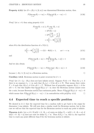
3.2.2 Path samples](https://image.slidesharecdn.com/edc87572-6bc2-40ac-a67c-f53bfedb3e6d-160930223103/85/tfg-28-320.jpg)
![CHAPTER 3. SIMULATIONS: RANDOM WALKS 24
Figure 3.5: Two different simulations for a 2D random walk. The particle (blue) will go up,
down, left or right with equal probability.
3.2.3 Code
We used a code in Java provided by Princeton:
public class randomWalk2 {
public static void main( String [ ] args ) {
int N = 60;
StdDraw . setXscale(−N, +N) ;
StdDraw . setYscale(−N, +N) ;
StdDraw . c l e a r (StdDraw .GRAY) ;
int x = 0 , y = 0;
int steps = 0;
while (Math . abs (x) < N && Math . abs (y) < N) {
StdDraw . setPenColor (StdDraw .WHITE) ;
StdDraw . f i l l e d S q u a r e (x , y , 0 . 4 5 ) ;
double r = Math . random ( ) ;
i f ( r < 0.25) x−−;
else i f ( r < 0.50) x++;
else i f ( r < 0.75) y−−;
else i f ( r < 1.00) y++;
steps++;
StdDraw . setPenColor (StdDraw .BLUE) ;
StdDraw . f i l l e d S q u a r e (x , y , . 4 5 ) ;
StdDraw . show ( 4 0 ) ;
}
StdOut . println ( ”Total steps = ” + steps ) ;
}
}
The functions StdDraw and StdOut are just for drawing and printing the results. They are](https://image.slidesharecdn.com/edc87572-6bc2-40ac-a67c-f53bfedb3e6d-160930223103/85/tfg-29-320.jpg)
![CHAPTER 3. SIMULATIONS: RANDOM WALKS 25
defined in other documents but they are not interesting for our purposes. The algorithm creates
a loop, for which in each step a random number r in the interval (0, 1] is created. The interval
is divided into four equal parts. Depending on the value of r the particle will go down, up, left
or right.
3.3 Three-dimensional random walk
The first two simulations in the section are identical as in the previous section, but for three-
dimensional random walks. The values for the first histogram are N = 60 and M = 50000 and
for the second histogram N = 1000 and M = 10000. The histograms are the following
Figure 3.6
As before, we could compute the probabilites an with the information in the plot
a2 ≈
8500
50000
= 0.17 (3.4)
a4 ≈
2000
50000
= 0.04 (3.5)
a6 ≈
1000
50000
= 0.02 (3.6)
. . . (3.7)
Next histogram is in log-log scale for better visualization, and the regression line has been
calculated](https://image.slidesharecdn.com/edc87572-6bc2-40ac-a67c-f53bfedb3e6d-160930223103/85/tfg-30-320.jpg)
![CHAPTER 3. SIMULATIONS: RANDOM WALKS 26
Figure 3.7: Plot and regression line y = mx + b with m = −0.24 and b = 3.24
Before we move on, let’s have a look at the regression lines for the 2D and 3D random walks.
For the 2D random walk we obtained y = −0.14x + 3.38 while for the 3D random walk y =
−0.24x + 3.24.
First we start with the similarities. They both have a negative slope and a positive intercept.
This all makes sense, a negative slope means that the number of particles that come back to
the origin after N steps is smaller than the number that come back after n steps, where N > n.
Alternatively, the more steps that a particle has been away from the origin, the less ‘probable’
it is to come back in the next step. For this reason, the intercept must be positive. Otherwise
it would lack of any physical sense as the number of steps would take negative values.
The big difference between them is the slope of the regression lines. For the 2D case we have
m = −0.14 and for the 3D m = −0.24 which is a difference close to 50%. This means that
the increment ∆N = N2 − N1, where N2 > N1, is smaller for 2D than for 3D. That is, the
histogram for 3D is more ‘heavy’ for small values of N and it decreases faster to 0 as N grows
than for the 2D case.
3.3.1 Code
The following script runs M different simulations of random walks of length at most N. For
every simulation when the random walk reaches 0 for the first time it stops the simulation and
keeps the number of steps in a vector v.
def SimRandomWalk3D(N=100,M=1000):
v=[]
for l in range (1 ,M) :
x=numpy . random . uniform (0 ,6 ,(N, 1 ) )
x[0]=0
i=1
k=0
sumax=1](https://image.slidesharecdn.com/edc87572-6bc2-40ac-a67c-f53bfedb3e6d-160930223103/85/tfg-31-320.jpg)
![CHAPTER 3. SIMULATIONS: RANDOM WALKS 27
sumay=1
sumaz=1
while (sumax!=0 or sumay!=0 or sumaz!=0) and i<N or k==0:
i f k==0:
k=1
sumax=0
sumay=0
i f x [ i ]>0 and x [ i ] <1:
sumax=sumax+1
i f x [ i ]>1 and x [ i ] <2:
sumax=sumax−1
i f x [ i ]>2 and x [ i ] <3:
sumay=sumay+1
i f x [ i ]>3 and x [ i ] <4:
sumay=sumay−1
i f x [ i ]>4 and x [ i ] <5:
sumaz=sumaz+1
i f x [ i ]>5 and x [ i ] <6:
sumaz=sumaz−1
i=i+1
i f sumax==0 and sumay==0 and sumaz==0:
v . append ( i −1)
return v
for plotting figure (3.6):
def freqHistogram3D (N=30,M=50000):
plt . h i s t (SimRandomWalk3D(2*N,M) , bins=N−1)
blue patch = mp. Patch ( color=’ blue ’ , l a b e l=’ Experimental frequencies ’ )
plt . legend ( handles =[ blue patch ] )
plt . xlabel ( ’N’ )
plt . ylabel ( ’ Frequency ’ )
and for plotting figure (3.7):
def freqHistogram3DLogLogLine (N=1000,M=10000):
bins=9
xam=[]
logn =[]
x = numpy . linspace (0 ,8 ,100)
X=l i s t (map(math . log , SimRandomWalk3D(2*N,M) ) )
(n , bins , patches ) = plt . h i s t (X, bins=numpy . arange ( bins ) , log=True )
blue patch = mp. Patch ( color=’ blue ’ , l a b e l=’ Experimental frequencies ’ )
plt . legend ( handles =[ blue patch ] )
plt . xlabel ( ’ log (N) ’ )
plt . ylabel ( ’ Frequency ’ )
for m in range ( 0 , 8 ) :
xam. append (0.5+m)
i f n [m]!=0:
logn . append (math . log10 (n [m] ) )
else :
logn . append (0)](https://image.slidesharecdn.com/edc87572-6bc2-40ac-a67c-f53bfedb3e6d-160930223103/85/tfg-32-320.jpg)
![CHAPTER 4. BROWNIAN MOTION 30
today trivial, it was far from trivial over 100 years ago. In fact, the atomistic hypothesis, that
is, the hypothesis that matter is grainy and cannot be continuously divided infinitely, was not
commonly accepted. Some scientists treated it as an unsupported working hypothesis and oth-
ers, including eminent figures as Wilhelm Ostwald, the 1909 Nobel Prize in chemistry, opposed
it vigorously.
Einstein and Smoluchowski claimed that this motion provided a proof of the existence of
molecules in the solvent and, what is more, that by observing the Brownian particles one
could get much insight into the properties of the molecules of the solvent. They observed that
the mean displacement of a particle (squared) was proportional to the duration of the obser-
vation, and that the proportionality constant was related to the so-called diffusion coefficient
D:
E[(Bt − B0)2
] = 2Dt, D =
KBT
γ
(4.1)
where KB is the Boltzmann constant, T the temperature and γ = 6πνR is the Stokes friction
coefficient for a spehere with radius R. These results rendered feasible many specific measures,
for example it was possible to experimentally determine the Avogadro constant.
It is interesting to know that explaining Brownian motion was not Einstein’s goal. He was
aiming to establish a relationship between the diffusion coefficient and the themperature, in
which he succeeded, but he also guessed what the thermal motion should look like. On the
contrary, Smoluchowski knew the experimental data on the Brownian motion very well and in-
tended to explain them. It is now clear that Smoluchowski obtained the results before Einsten,
but decided to publish them after he was impressed by Einstein work.
These papers have also answered several other questions. First, they provided a microscopical
explanation of diffusion (molecules of the substance that diffuses are ‘pulled through’ by the
collisions with the molecules in the solvent), second, they derived an equation known today
as the diffusion equation, and third they explained why all other attemps in describing the
Brownian motion in terms of velocities had failed. Smoluchowski noticed that displacements
of Brownian particles seen in a microscope resulted from a huge number of collisions with the
molecules of the solvent: the displacements were averaged over many such collisions. The time
between two consecutive collisions is much shorter that we can now, in the 21t
h century, ob-
serve. At any two observed zigzags there are many other zigzags that have happened and we
have failed to observe.
There is an important remark to do here. The Newtonian dynamics, commonly used in Smolu-
chowski times and today for explaining a large array of phenomena, says that the trajectory
of any particle can be described by means of a certain differential equation. To write down
this equation, you need to know all the forces acting on this particle. The forces may be
changing but as long as these changes are smooth, the trajectory of the particle will also be
smooth. Smoluchowski revolutionary point of view was that Brownian motion was not smooth,
therefore challenging a ‘sacred’ canon of Physics back then. This was truly a deviation of a
well-established paradigm, but it was succesful in explaning an experiment that other theories
could not explain. The diffusion equation mentioned above does not aim to explain perfectly
the behaviour of a single particle, but rather the behaviour a large enough amount of particles,
for example a drop of ink in a water tank. While the motion of a single particle may be erratic
and awkward, the collective behaviour can be quite decent and predictible.
This is a totally new approach in Physics, that changes from deterministic to probabilistic.
The works of Einstein and Smoluchowski have become one of the cornerstones of Probability
Calculus and the theory of Stochastic Processes](https://image.slidesharecdn.com/edc87572-6bc2-40ac-a67c-f53bfedb3e6d-160930223103/85/tfg-35-320.jpg)
![CHAPTER 4. BROWNIAN MOTION 36
ˆ Neighbourhood recurrent, if, almost surely, for every x ∈ Rd
and ε > 0, there exists
a (random) sequence tn → ∞ such that X(tn) ∈ B(x, ε) for all n ∈ N.
ˆ Transient, if it converges to infinity almost surely
Before we can prove the Brownian motion recurrence, we will need some understanding on
harmonic functions. Especifically, we will have a look at the Dirichlet Problem. This problem
raises the following question: given a continuous function ϕ on the boundary of a domain, is
there a function u such that u(x) = ϕ(x) in the boundary of the domain and such that u(x)
is harmonic inside the domain? That is, we are trying to extend the definition of ϕ in the
boundary to a ’nice’ function in the whole domain. Gauss posed this problem in 1840, and
he thought he proved there was always a solution, but his reasoning was wrong and Zaremba
in 1911 gave counterexamples. However, if the domain is ’nice enough’ (see Poincar´e cone
condition below) there is always a solution.
The Dirichlet Problem can be solved purely by analytical tools. We will however solve it by
probabilistic means.
Definition 4.3.6. Let U be a domain, i.e., a connected open set U ⊂ Rd
. A function ϕ : U → R
is harmonic (on U) if it is twice continuously differentiable and, for any x ∈ U,
∆u(x) :=
d
j=1
∂2
u
∂x2
j
(x) = 0 (4.33)
Definition 4.3.7. Let U ⊂ Rd
be a domain. We say that U satisfies the Poincar´e cone
condition at x ∈ ∂U if there exists a cone V based at x with opening angle α > 0, and h > 0
such that V ∩ B(x, h) ⊂ Uc
.
Definition 4.3.8. A random variable T with values in [0, ∞], defined on a probability space
with filtration (F(t) : t ≥ 0) is called a stopping time with respect to (F(t) : t ≥ 0) if
{ω : T(ω) ≤ t} ∈ F(t) for every t ≥ 0.
Remark 4.3.2. Speaking intuitively, for T to be a stopping time, it should be possible to
decide whether or not {T ≤ t} has occurred on the basis of the knowledge of F(t).
Definition 4.3.9. Suppose that X = (Xt : t ≥ 0) is a stochastic process on a probability space
(Ω, F, P) with natural filtration {F(t) : t ≥ 0)}. For any t ≥ 0 we can define the sigma algebra
F(t+
) to be the intersection of all Fs for s ≥ t. Then for any stopping time τ on Ω we can
define
F(τ) = {A ∈ F : {τ = t} ∩ A ∈ F(t+
), ∀t ≥ 0} (4.34)
Then X is said to have the strong Markov property if, for each stopping time τ, conditioned on
the event {τ < ∞}, we have that for each t ≥ 0, Xτ+t is independent of F(τ) given Xτ .
Theorem 4.3.1 (Dirichlet Problem). Suppose U ∈ Rd
is a bounded domain such that every
boundary point satisfies the Poincar´e cone condition, and suppose ϕ is a continuous function
on ∂U. Let τ(∂U) = inf{t > 0 : B(t) ∈ ∂U}, which is an almost surely finite stopping time.
Then the function u : ¯U → R given by
u(x) = E(ϕ(B(τ(∂U)))|B(0) = x), for x ∈ U (4.35)
is the unique continuous function harmonic on U with u(x) = ϕ(x) for all x ∈ ∂U.
Remark 4.3.3. If the Poincar´e cone condition holds at every boundary point, one can simulate
the solution of the Dirichlet problem by running many independent Brownian motions, starting
in x ∈ U until they hit the boundary of U and letting u(x) be the average of the values of ϕ
on the hitting points.](https://image.slidesharecdn.com/edc87572-6bc2-40ac-a67c-f53bfedb3e6d-160930223103/85/tfg-41-320.jpg)
![CHAPTER 4. BROWNIAN MOTION 37
With this result in mind, let’s find explicit solutions u : cl A → R of the Dirichlet problem on
an annulus A = {x ∈ Rd
: r < |x| < R}. The reason to study this case is that the recurrence
problem will be a particular case of this solution. It is first reasonable to assume that u is
spherically symmetric, i.e. there is a function ψ : [r, R] → R such that u(x) = ψ(|x|2
). We can
express derivatives of u in terms of ψ as
∂iψ(|x|2
) = ψ (|x|2
)2xi (4.36)
∂iiψ(|x|2
) = ψ (|x|2
)4x2
i + 2ψ (|x|2
) (4.37)
Therefore, ∆u = 0 means
0 =
d
i=1
ψ (|x|2
)4x2
i + 2ψ (|x|2
) = 4|x|2
ψ (|x|2
) + 2dψ (|x|2
)
Letting y = |x|2
> 0 we can write this as
ψ (y) = −
d
2y
ψ (y)
This is solved by every ψ satisfying ψ (y) = Cy−d/2
and thus ∆u = 0 holds on {|x| = 0} for
u(x) =
|x| if d = 1
2 log |x| if d = 2
|x|2−d
if d = 3
(4.38)
We write u(r) for the value of u(x) for all x ∈ ∂B(0, r). Now define stopping times
Tr = τ(∂B(0, r)) = inf{t > 0 : |B(t)| = r} for r > 0 (4.39)
and denote by T = Tr ∧ TR the first exit time from A. By the Dirichlet Problem Theorem
(4.3.1) we have
u(x) = E(u(B(T))|B(0) = x) = u(r)P(Tr < TR|B(0) = x) + u(R)(1 − P(Tr < TR))
which can be solved
P(Tr < TR|B(0) = x) =
u(R) − u(x)
u(R) − u(r)
(4.40)
This formula gives an explicit computation of the probability that the Brownian motion hits
∂B(0, r) before ∂B(0, R). We have just proved the following theorem
Theorem 4.3.2. Suppose {B(t) : t ≥ 0} is a Brownian motion in dimension d ≥ 1 started in
x ∈ A, which is an open annulus A with radii 0 < r < R < ∞. Then,
P(Tr < TR|B(0) = x) =
R − |x|
R − r
if d = 1
log R − log |x|
log R − log r
if d = 2
R2−d
− |x|2−d
R2−d − r2−d
if d ≥ 3
(4.41)
if we take the limit R → ∞ we get the following corollary](https://image.slidesharecdn.com/edc87572-6bc2-40ac-a67c-f53bfedb3e6d-160930223103/85/tfg-42-320.jpg)
![CHAPTER 4. BROWNIAN MOTION 42
where we have used in the second step property 4.3.1. Hence we obtain
P( max
0≤s≤h
Bs > 0) = 1 (4.57)
Finally, if we notice that
P( min
0≤s≤h
Bs < 0) = P( max
0≤s≤h
−Bs > 0) (4.58)
we can use the same arguments and get
P( min
0≤s≤h
Bs < 0) = 1 (4.59)
4.5 Other properties of Brownian motion
In this section we will show some interesting properties of the Brownian motion that we will
use in the next sections.
4.5.1 Quadratic variation
Let πn : 0 = t0 < t1 < · · · < tn = T be a partition on [0, T]. For a smooth function we have the
following proposition.
Proposition 4.5.1. Let (πn) a sequence of refining partitions with mesh(πn) → 0 on [0, T] and
f ∈ C1
. Then
n
i=1
(f(ti) − f(ti−1))2
→ 0, as n → ∞ (4.60)
Proof. We can use the mean value theorem, since f ∈ C1
.
n
i=1
(f(ti) − f(ti−1))2
=
n
i=1
f(ξi)2
(ti − ti−1)2
≤ max
0≤i≤n
(f(ξi)2
)
n
i=1
(ti − ti−1)2
≤ max
0≤i≤n
(f(ξi)2
)mesh(πn)
n
i=1
(ti − ti−1)
= Cmesh(πn)T → 0
where ξi ∈ (ti, ti+1).
However, for the Brownian motion we have a different result.
Proposition 4.5.2. Let (πn) be a sequence of refining partitions with mesh(πn) → 0 on [0, T]
and B = (Bt, t ≥ 0) a Brownian motion. Then
Qn =
n
i=1
(B(ti) − B(ti−1))2
=
n
i=1
(∆iB)2 L2
−→ T, as n → ∞ (4.61)
and thus it converges also in probability.](https://image.slidesharecdn.com/edc87572-6bc2-40ac-a67c-f53bfedb3e6d-160930223103/85/tfg-47-320.jpg)
![CHAPTER 4. BROWNIAN MOTION 43
Proof. We want to see that
E[(Qn − T)2
] −→ 0, as n → ∞ (4.62)
First thing to notice is that E(Qn) = T. Indeed, since ∆iB ∼ N(0, ti − ti−1) we have
E(Qn) = E
n
i=1
(B(ti) − B(ti−1))2
=
n
i=1
E(B(ti) − B(ti−1))2
=
n
i=1
(ti − ti−1) = T (4.63)
From here we get the following expression
E[(Qn − T)2
] = E[(Qn − E(Qn))2
] = V ar(Qn) (4.64)
which can be written using the identity V ar(X) = E(X2
) − E(X)2
and the fact that the
increments ∆iB are independent as
V ar(Qn) =
n
i=1
V ar (∆iB)2
=
n
i=1
E(∆iB)4
− ∆2
i (4.65)
where ∆i = ti − ti−1.
It is well know that for a N(0, 1) random variable B1, EB4
1 = 3, then
E(∆iB)4
= E (∆i)1/2
B1
4
= 3∆2
i (4.66)
which implies
V ar(Qn) = 2
n
i=1
∆2
i (4.67)
thus if
mesh(πn) = max
i=1,...,n
∆i → 0 (4.68)
we obtain that
E[(Qn − T)2
] = V ar(Qn) ≤ 2mesh(πn)
n
i=1
∆i = 2Tmesh(πn) → 0 (4.69)
4.5.2 Unbounded variation
Proposition 4.5.3. Let B = (Bt, t ≥ 0) be a Brownian motion, then almost surely
sup
πn
n
i=1
|∆iB| = +∞ (4.70)
that is
P ω ∈ Ω : sup
πn
n
i=1
|∆iB(ω)| = +∞ = 1 (4.71)
where we take the suprema over all partitions πn of [0, T], where ∆iB = Bti
− Bti−1
.](https://image.slidesharecdn.com/edc87572-6bc2-40ac-a67c-f53bfedb3e6d-160930223103/85/tfg-48-320.jpg)
![CHAPTER 4. BROWNIAN MOTION 44
Proof. Let
A = ω ∈ Ω : sup
π
n
i=1
|∆iB(ω)| < C(ω) < ∞ (4.72)
and assume that
P(A) > 0 (4.73)
and consider a sequence of partitions (πn) such that mesh(πn) → 0. From proposition 4.5.2
Qn =
n
i=1
(B(ti) − B(ti−1))2 L2
−→ T (4.74)
which means that there is a subsequence of partitions, σnk
such that
Qnk
a.s
−→ T > 0 (4.75)
and thus
P ω ∈ Ω : lim
k
Qnk
(ω) = T = 1 (4.76)
which implies
P ω ∈ Ω : lim
k
Qnk
(ω) = T = 0 (4.77)
On the other hand for ω ∈ A we have
Qn(ω) =
n
i=1
(B(ti) − B(ti−1))2
≤ max
i=1,...,n
|∆iB(ω)|
n
i=1
∆iB
≤ C(ω) max
i=1,...,n
|∆iB(ω)| → 0
because Bt is continuous and then uniformly continuous on [0, T]. Hence
P ω ∈ Ω : lim
k
Qnk
(ω) = 0 = T > 0 (4.78)
in contradiction with (4.77).](https://image.slidesharecdn.com/edc87572-6bc2-40ac-a67c-f53bfedb3e6d-160930223103/85/tfg-49-320.jpg)
![Chapter 5
Simulations: Brownian Motion
In this section we want to simulate a Brownian Motion. For that, some prior knowledge of
numerical integration of stochastic differential equations will be needed. The tools developed
in this chapter will let us indeed integrate more complex SDEs than the Brownian motion.
5.1 Numerical integration of stochastic differential equa-
tions with Gaussian white noise
Let us start with a simple stochastic differential equation:
˙x(t) = f(t) + ξ(t) (5.1)
where f(t) is a deterministic function and ξ(t) is a Gaussian white noise, i.e., ξ(t) ∼ N(0, 1).
If we integrate we get
x(t) = x(0) +
t
0
f(s)ds +
t
0
ξ(s)ds (5.2)
which can be written as
x(t) = x(0) + F(t) + B(t) (5.3)
where F(t) =
t
0
f(s)ds and B(t) is the brownian motion. This expression indicates that x(t)
is a Gaussian process whose mean and correlation are given by
E(x(t)) = x(0) + F(t) (5.4)
E(x(t)x(t )) = [x(0) + F(t)][x(0) + F(t )] + min(t, t ) (5.5)
Now we will focus on a numerical solution, rather than solving the equations. Our final aim will
be to be able to generate trajectories, that is, we want to obtain x(t) at discrete time intervals
x(t + h) = x(t) +
t+h
t
˙x(s)ds = x(t) +
t+h
t
f(s)ds +
t+h
t
ξ(s)ds (5.6)
Introducing
fh(t) :=
t+h
t
f(s)ds (5.7)
and
wh(t) :=
t+h
t
ξ(s)ds = B(t + h) − B(t) (5.8)
45](https://image.slidesharecdn.com/edc87572-6bc2-40ac-a67c-f53bfedb3e6d-160930223103/85/tfg-50-320.jpg)
![CHAPTER 5. SIMULATIONS: BROWNIAN MOTION 47
Euler-Maruyama method
We start with the equation
˙x(t) = q(x) + g(x)ξ(t) (5.19)
For additive noise, g(x) does not depends on x, and g(x) =
√
D with D being a constant, then
the Euler-Maruyama method for stochastic differential equations is given by
x(t + h) = x(t) + hq(x(ti)) +
√
Dhu(t) + O[h3/2
] (5.20)
As we need Stratonovich calculus to show the derivation of this formula, we will just state it
and use it later.
5.1.1 Runge-Kutta-Type methods
Equation (5.16) is enough to simulate the pure brownian motion, but in this section we will
develop a more advance method for integrating other kind of stochastic differential equations.
We start with the equation (5.19) and we would like to develop a method inspired by the
Runge-Kutta methods used for numerical integration of ordinary differential equations. There
is a large family of Runge-Kutta methods. Here, we focus on one of the simplest methods
of this family, known as the Heun method, which is of second order. We start revisiting the
deduction of the Heun numerical algorithm for ordinary differential equations and then we
extend the ideas to the case of stochastic differential equations. Let’s start considering the
ordinary differential equation
˙x(t) = q(t, x) (5.21)
where, in general, q(t, x(t)) is a nonlinear function of x(t) which can also depend on the time
explicitly. We start by applying the Euler method to integrate this equation:
x(ti+1) = x(ti) + hq(ti, x(ti)) + O[h2
] (5.22)
This is an explicit map since the right-hand side depends only on known values of the variable
x at previous times, while the unknown variable x(ti+1) is explicitly isolated in the left-hand
side. In fact, (5.22) corresponds to the explicit Euler, also called the forward Euler method.
There is also an implicit Euler method (also called the backward Euler method) to integrate
the same equation, which is given by
x(ti+1) = x(ti) + hq(ti+1, x(ti+1)) + O[h2
] (5.23)
The implicit Euler method is more stable than the explicit one but it has the disadvantage
that, in general, it is difficult to invert the function q(t, x(ti)) appearing on the right-hand side
so that one could get an explicit expression for x(ti+1) as a function of x(ti). Finally, there is
a semi-implicit Euler method that combines both approaches and which is of order O[h3
]. It is
given by
x(ti+1) = x(ti) +
h
2
[q(ti, x(ti)) + hq(ti+1, x(ti+1))] + O[h3
] (5.24)
This method suffers from the same inconvenience as the implicit Euler: the recurrence relation
is given by an implicit map. A way to circumvent this inconvenience is to replace x(ti+1) on
the right-hand side by the value obtained by using the explicit Euler method (5.22), namely by
x(ti) + hq(t, x(ti)):
x(ti+1) = x(ti) +
h
2
[q(ti, x(ti)) + q(ti+1, x(ti) + hq(t, x(ti)))] + O[h3
] (5.25)](https://image.slidesharecdn.com/edc87572-6bc2-40ac-a67c-f53bfedb3e6d-160930223103/85/tfg-52-320.jpg)
![CHAPTER 5. SIMULATIONS: BROWNIAN MOTION 48
This is the Heun method that is usually written as
k = hq(t, x(ti)) (5.26)
x(ti+1) = x(ti) +
h
2
[q(ti, x(ti)) + q(ti+1, x(ti) + k)] (5.27)
We now apply the same ideas to a stochastic differential equation with white noise (5.19). Let
us start with a semi-implicit version of Euler’s method given by (5.20)
x(ti+1) = x(ti) +
h
2
[q(ti, x(ti)) + q(ti+1, x(ti+1))] +
√
hui
2
[q(ti, x(ti)) + q(ti+1, x(ti+1))] (5.28)
And now replace x(ti) on the right- hand side by the prediction given by the Euler-Maruyama
algorithm (5.20). The resulting algorithm can be written as
k = hq(t, x(ti)) (5.29)
l =
√
huig(t, x(ti)) (5.30)
x(ti+1) = x(ti) +
h
2
[q(ti, x(ti)) + q(ti+1, x(ti) + k + l)] +
√
hui
2
[g(ti, x(ti)) + g(ti+1, x(ti) + k + l)]
(5.31)
This is known as the stochastic Heun method. Notice that for the pure Brownian motion one
has q(t, x(ti)) = 0 and g(t, x(ti)) = 1 which converges to the simple formula (5.18). 1
5.1.2 Simulations
In this section we will simulate the Brownian motion and will see how long it takes until it
reaches back the value a = 0.1, that is, for which t = 0 we have that Bt = 0.5. The reason
why we do not take a = 0 is not arbitrary. In the discrete case for a random walk there was
no problem in taking a = 0, but for a Brownian motion some issues arise. The most important
is regarding property 4.4.1. Since we know that next to 0 there are infinite points t such that
Bt = 0, it doesn’t make a lot of sense to simulate this case. For this reason we have decided to
take a = 0, for example a = 0.1.
We will gather the results in a histogram. The simulations will be somewhat similar to those for
the random walk. However, one big difference to notice, is that Brownian motion is a continuous
function while a random walk is a discrete one. Another to notice is that the stopping time Ta
has a continuous density, which implies that the probability of every single point is 0. Taking
into account these differences, we cannot make histograms for Brownian motion that reaches a
point after N steps, because every step is infinitely small (theoretically, although in simulations
we will discretize). For this reason counting how many come back after N steps does not make
conceptual sense and, therefore, the bins in the histogram will represent a time interval rather
than a time point. The following simulation contains 106
different points, calculated according
to the formula
x(t0) = 0 (5.32)
x(ti+1) = x(ti) +
√
hui (5.33)
1
These more sophisticated methods were developed in the thesis in order to simulate some more complex
stochastic differential equations than the pure Brownian motion. However, because of lack of time and space
we decided to give priority to other topics.](https://image.slidesharecdn.com/edc87572-6bc2-40ac-a67c-f53bfedb3e6d-160930223103/85/tfg-53-320.jpg)
![CHAPTER 5. SIMULATIONS: BROWNIAN MOTION 49
A total of 105
simulations were run. For practical reasons, the bins of the histograms represent
intervals in log(t) rather than just t. We have also ploted the theoretical density obtained in
Theorem 4.4.1 to compare results. First, we need to do a change of variable for the density,
because we are plotting the density of Y = g(Ta) = log(Ta) instead of the density of Ta:
fY (y) = fa(g−1
(y))|(g−1
) (y)|1(−∞,∞)
=
a
√
2πey
e− a2
2ey
This is the result we obtain:
Figure 5.1: Shows the relative number of particles that reached Bt = 0.5 for the first time at
time log(t).
First thing to notice is that theoretical results and empirical results do not match as perfectly
as in the random walk. We observe that for several values the experimental data is lightly large
than the predicted value. The reason for this discrepancy is that we plotted the histogram for a
fixed number of bins and selected the option ‘normed=True’, that is, the sum of all bins is equal
to 1. For a perfect match to the theoretical curve, we should consider every bin from −∞ to
∞. However, we plotted the high probability bins and, appart from those small discrepancies,
we observe a quite good match.
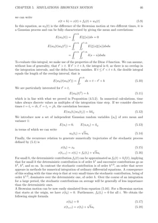
5.1.3 Code
We will now write a code to plot four different Brownian motion samples, using the equation
(5.16). In our case
def plotBrownianMotion (h=1, l =1000):
x=[]
x . append (0)
y=[]
y . append (0)](https://image.slidesharecdn.com/edc87572-6bc2-40ac-a67c-f53bfedb3e6d-160930223103/85/tfg-54-320.jpg)
![CHAPTER 5. SIMULATIONS: BROWNIAN MOTION 50
z =[]
z . append (0)
v=[]
v . append (0)
for i in range (0 , int ( l /h ) ) :
x . append (x [ i ]+np . sqrt (h)*np . random . normal ( loc =0.0 , s c a l e =1.0))
plt . plot (x , c=’b ’ )
for i in range (0 , int ( l /h ) ) :
y . append (y [ i ]+np . sqrt (h)*np . random . normal ( loc =0.0 , s c a l e =1.0))
plt . plot (y , c=’ r ’ )
for i in range (0 , int ( l /h ) ) :
z . append ( z [ i ]+np . sqrt (h)*np . random . normal ( loc =0.0 , s c a l e =1.0))
plt . plot ( z , c=’y ’ )
for i in range (0 , int ( l /h ) ) :
v . append (v [ i ]+np . sqrt (h)*np . random . normal ( loc =0.0 , s c a l e =1.0))
plt . plot (v , c=’ g ’ )
plt . show ()
This will alow us to draw Brownian motion samples. The same code is valid for plotting
Brownian motion samples in 2D, only changing plt.plot(x,c=’b’) for plt.plot(x,y,c=’b’) For
plotting the histogram 5.1 we have written the following code
def simBrownianMotion (h=1, l =10000,N=1000):
v=[]
for n in range (1 ,N) :
#x=numpy . random . normal (0 ,1 ,3)
i=0
suma=0
sumaa=0
while (0.5 −sumaa)*(0.5 −suma)>=0 and i<l :
sumaa=suma
suma=suma+np . sqrt (h)*np . random . normal (0 ,1)
i=i+h
i f (0.5 −sumaa)*(0.5 −suma)<0:
v . append ( i−h)
return v
t1 = np . arange (−6, 10 , 0.1)
plt . plot ( t1 ,
np . exp ( −0.5**2/(2*np . exp ( t1 )))* 0.5/ np . sqrt (2*math . pi *np . exp ( t1 ) ) )
def freqHistogramBrownian (h=0.01 , l =1000,N=100000):
bins=13
X=l i s t (map( log , simBrownianMotion (h , l ,N) ) )
(n , bins , patches ) = plt . h i s t (X, bins =[−5,−4.5,−4,−3.5,−3,−2.5,
−2 , −1.5 , −1 , −0.5 ,0 ,0.5 ,1 ,
1. 5 , 2 , 2.5 ,3 ,3 .5 , 4 , 4.5 ,5 ,
5 . 5 , 6 , 6 . 5 , 7 , 7 . 5 , 8 ] , normed=True )
plt . xlabel ( ’ log ( t ) ’ )](https://image.slidesharecdn.com/edc87572-6bc2-40ac-a67c-f53bfedb3e6d-160930223103/85/tfg-55-320.jpg)
![CHAPTER 5. SIMULATIONS: BROWNIAN MOTION 52
example, and we know that the extension will be u(x, y) = f(x, y) = x + y for all (x, y) ∈ U, so
we can verify if the algorithm works. A Brownian motion will start at 0 and will at some point
cross the boundary. The average of all the points at which the simulations crosses the boundary
will give us the value of f(x, y). In this example we will calculate u(0, 0). Intuitively, we would
expect that u(0, 0) = 0, because of the symmetry of this case. For every Brownian motion
that crosses the boundary at some point (x, y) we would expect another Brownian motion to
cross it at the point (−x, −y), so the average of all this points looks like it should be 0. We
will run 105
Brownian motions starting at (x, y) = (0, 0) to compute this point. The result is
u(0, 0) = 0.0176. The code we used is the following.
5.2.1 Code
def f (x , y ) :
return x+y
def d i r i c h l e t (h=1, l =10000,N=100000,x=0,y=0):
v=[]
for n in range (1 ,N) :
#x=numpy . random . normal (0 ,1 ,3)
i=1
sumax=x
sumaax=x
sumay=y
sumaay=y
while (10−sumaax)*(10−sumax)>=0 and (10−sumaay)*(10−sumay)>=0
and (−10−sumaax)*(−10−sumax)>=0 and (−10−sumaay)*(−10−sumay)>=0
and i<l :
sumaax=sumax
sumax=sumax+np . sqrt (h)*np . random . normal (0 ,1)
sumaay=sumay
sumay=sumay+np . sqrt (h)*np . random . normal (0 ,1)
i=i+1
i f sumax*sumaax<0 or sumay*sumaay<0:
v . append ( f (sumax , sumay ))
print (sum(v)/ len (v ))
return sum(v)/ len (v)
We compute a two dimensional Brownian motion in a similar way than the one dimensional
case. In every step we compute the two variables x and y as
x(t0) = 0 (5.34)
y(t0) = 0 (5.35)
x(ti+1) = x(ti) +
√
hui,1 (5.36)
y(ti+1) = y(ti) +
√
hui,2 (5.37)](https://image.slidesharecdn.com/edc87572-6bc2-40ac-a67c-f53bfedb3e6d-160930223103/85/tfg-57-320.jpg)
![Chapter 6
Stochastic integrals
In this chapter we will try to develop an integral for stochastic processes. In particular, we are
interested in the integral
t
0
f(s)dBs(ω), where (Bt(ω), t ≥ 0) is a given Brownian sample path
and f is a deterministic function or the sample path of a stochastic process. This integrals may
seem a little too abstract, but they are very useful tools to model different situations. As an
example of application, we will see that they are necessary when developing the next chapter:
Stochastic calculus in Finance. Our first approach will be the Riemann-Stieltjes integral, but
as we will soon see this has a limited use, and another approach will be needed.
6.1 Riemann-Stieltjes integral
We will not go into deep detail in this section, as its only purpose is the motivation for our
next section where we will build the Itˆo integral.
From now let’s consider τn a partition τn : {0 = t0 < t1 < . . . < tn = T} over the interval [0, T]
and σn an intermediate partition of τn:
σn : ti−1 ≤ yi ≤ ti for i = 1, . . . , n (6.1)
and let
∆ig = g(ti) − g(ti−1), i = 1, . . . , n (6.2)
Definition 6.1.1. Let f and g two real-valued functions on [0, 1]. The Riemann-Stieltjes sum
corresponding to τn and σn is given by
Sn = Sn(τn, σn) =
n
i=1
f(yi)∆ig =
n
i=1
f(yi)(g(ti) − g(ti−1)) (6.3)
Definition 6.1.2. If the limit
S = lim
n→∞
Sn = lim
n→∞
n
i=1
f(yi)∆ig (6.4)
exists as mesh(πn) = max(|ti − ti−1|, i = 1, . . . , n) → 0 and S is independent of the choice of
the partitions σn, then S is called the Riemann-Stieltjes integral of f with respect to g on [0, 1]
and we write
S =
T
0
f(t)dg(t) (6.5)
So now we can consider the previous integral for stochastic processes. However, the following
theorem shows its limitations.
53](https://image.slidesharecdn.com/edc87572-6bc2-40ac-a67c-f53bfedb3e6d-160930223103/85/tfg-58-320.jpg)
![CHAPTER 6. STOCHASTIC INTEGRALS 54
Theorem 6.1.1. Let g(t) be a continuous function on [0, 1] and (πn) a sequence of refining
partitions of [0, 1] such that its norm tends to zero, then the Riemann-Stieltjes integral
T
0
fdg = lim
n
ti,ti+1∈πn
f(yi)(g(ti) − g(ti−1)) (6.6)
exists and is finite for all f ∈ C([0, 1]) ⇐⇒ g has bounded variation.
Corollary 6.1.1. Let B = (Bt, t ≥ 0) be a Brownian motion, then ∃f ∈ C([0, 1]) such that
T
0
f(t)dBt(ω) does not exist in the Riemann-Stieltjes integral.
Proof. We know from proposition 4.5.3 that Brownian motion has unbounded variation. Taking
g = B a Brownian motion from theorem 6.1.1 we get that there exists f such that
T
0
f(t)dB(ω)
is not well defined in the Riemann-Stieltjes sense.
Indeed, one does not need uncommon functions f for the previous integral not to exist. For ex-
ample, take
T
0
Bt(ω)dBt(ω). It can be shown that this integral does not exist in the Riemann-
Stieltjes sense.
Example 6.1.1. The integral
T
0
Bt(ω)dBt(ω) is not well defined in the Riemann-Stieltjes
sense. Let (πn) a sequence of refining partitions such that Qn → T almost surely. We know
such sequence exist from proposition 4.5.2. Assume the integral is well defined, then the limits
lim
n
n
i=1
Bti
(ω)(Bti+1
(ω) − Bti
(ω)), lim
n
n
i=1
Bti+1(ω)(Bti+1
(ω) − Bti
(ω)) (6.7)
exist and they are equal, which means that the difference is equal to 0
lim
n
n
i=1
Bti
(ω)(Bti+1
(ω) − Bti
(ω)) − Bti+1(ω)(Bti+1
(ω) − Bti
(ω)) = 0 (6.8)
but if one rearranges terms the previous sum becomes
0 = lim
n
n
i=1
(∆iB)2
= lim
n
Qn(ω) (6.9)
and using proposition 4.5.2 one obtains
lim
n
Qn → T (6.10)
in contradiction with the fact that Qn(ω) ≡ 0.
6.2 The Itˆo integral for simple processes
The previous section served as motivation to show the limitations of the Riemann-Stieltjes
integral. At first glance it may seem that it is the most natural definition for stochastic integrals,
but we saw that some simple integrals made no sense in the Riemann-Stieltjes sense. For this
reason, we will develop more advanced tools.](https://image.slidesharecdn.com/edc87572-6bc2-40ac-a67c-f53bfedb3e6d-160930223103/85/tfg-59-320.jpg)
![CHAPTER 6. STOCHASTIC INTEGRALS 55
Definition 6.2.1. The stochastic process C = (Ct, t ∈ [0, T]) is said to be simple if it satisfies
the following properties:
There exists a partition
τn : 0 = t0 < t1 < · · · < tn−1 < tn = T
and a sequence (Zi, i = 1, . . . , n) of random variables such that
Ct =
Zn, if t = T
Zi, if ti−1 ≤ t < ti, i = 1, . . . , n
The sequence (Zi) is adapted to (Fti−1
, i = 1, . . . , n),i.e., Zi is a ‘function’ of Brownian motion
up to time ti−1, and satisfies E(Z2
i ) < ∞ for all i.
Definition 6.2.2. Let C = (Ct, t ∈ [0, T) be a simple stochastic process on [0, T], τn : 0 = t0 <
t1 < · · · < tn−1 < tn = T a partition and B = (Bt, t ≥ 0) a Brownian motion.
The Itˆo stochastic integral of a simple process on [0, T] is given by:
T
0
CsdBs :=
n
i=1
Cti−1
(Bti
− Bti−1
) =
n
i=1
Zi∆iB (6.11)
The Itˆo stochastic integral of a simple process on [0, t], for tk−1 ≤ t ≤ tk is given by:
t
0
CsdBs :=
T
0
CsI[0,t](s)dBs =
k−1
i=1
Zi∆iB + Zk(Bt − Btk−1) (6.12)
6.3 The general Itˆo integral
From now on, we will assume that the process C = (Ct, t ∈ [0, T]) serves as the integrand of
the Itˆo stochastic integral and that the following conditions are satisfied:
ˆ C is adapted to Brownian motion on [0, T], i.e., Ct only depends on Bs, s ≤ t.
ˆ The integral
T
0
E(C2
s )ds is finite.
Remark 6.3.1. For a process C satisfying the assumptions one can find a sequence (C(n)
) of
simple processes such that
T
0
E(Cs − C(n)
s )2
ds → 0
This means that the processes (C(n)
) converge in a mean square sense to the process C. The
fact of (C(n)
) being a simple process means that we can evaluate all Itˆo stochastic integrals
It(C(n)
). Furthermore, it can be shown that the sequence It(C(n)
) converges in the mean square
sense to an unique limit process, say It(C), i.e.,
E( sup
0≤t≤T
[It(C) − It(C(n)
)]2
) → 0 (6.13)
Definition 6.3.1. The mean square limit It(C) is called the Itˆo stochastic integral of C. It is
denoted by
It(C) =
t
0
CsdBs, t ∈ [0, T] (6.14)
For a simple process C, the Itˆo stochastic integral has the Riemann-Stieltjes sum representation.](https://image.slidesharecdn.com/edc87572-6bc2-40ac-a67c-f53bfedb3e6d-160930223103/85/tfg-60-320.jpg)
![CHAPTER 6. STOCHASTIC INTEGRALS 57
Example 6.5.1. Consider a geometric Brownian motion Xt, which is given by
Xt = f(t, Bt) = X0e(c−1
2
σ2)t+σBt
(6.22)
where X0 is a random variable independent of the Brownian motion. If we apply formula (6.20)
we obtain that Xt satisfies
Xt − X0 = c
t
0
Xsds + σ
t
0
XsdBs (6.23)
6.6 Extension II of the Itˆo formula
We now consider a more general case than the I extension, where we have processes f(t, Xt)
and Xt is an Itˆo process. The reason why we are introducing these extensions of the Itˆo formula
is because we will need to use them in the next chapter.
Definition 6.6.1. A stochastic process Xt is called an Itˆo process if there are processes A(1)
and A(2)
adapted to Brownian motion Bt, and a random variable X0 such that Xt can be
written as.
Xt = X0 +
t
0
A(1)
s ds +
t
0
A(2)
s dBs (6.24)
Remark 6.6.1. One can show that the A(1)
and A(2)
are uniquely determined.
Using arguments similar to those used for the simple Itˆo formula one can arrive to the following
more general Itˆo formula:
Theorem 6.6.1. Let Xt be an Itˆo process and f ∈ C1,2
([0, ∞) × R). Then
f(t, XT ) − f(s, Xs) = (6.25)
=
t
a
f1(s, Xs) + A(1)
s f2(s, Xs) +
1
2
(A2
s)2
f22(s, Xs) ds +
t
a
A(2)
s f2(s, Xs)dBs (6.26)
where fi and fij represent the partial derivatives of f.
6.7 Stratonovich integral
It is useful to notice that the Itˆo integral is not the only possible integral for stochastic pro-
cesses, but rather just a member of a big family. The Itˆo integral has some nice mathematical
properties, but the classical chain rule does not apply. Instead, we need to use Itˆo’s formula.
For some applications it comes more handy to have an integral for which classical chain rule
applies, but the price we have to pay is some of the nice properties that the Itˆo integral has.
We start in the case that the integrand process is of the form f(Bt) where (Bt, t ≥ 0) is a
Brownian motion and f is a twice differentiable function on [0, T]. Let
ˆSn =
n
i=1
f(Byi
)∆iB (6.27)
where
∆iB = Bti
− Bti−1
, yi =
ti−1 + ti
2
, i = 1, . . . , n (6.28)
One can show that the Riemann-Stieltjes sums ˆSn exist if mesh(πn) → 0](https://image.slidesharecdn.com/edc87572-6bc2-40ac-a67c-f53bfedb3e6d-160930223103/85/tfg-62-320.jpg)
![CHAPTER 6. STOCHASTIC INTEGRALS 58
Definition 6.7.1. The unique mean square limit ST (f(B)) of the Riemann-Stieltjes sums ˆSn
exists if
T
0
E(f2
(Bt))dt < ∞. This limit is called the Stratonovich stochastic integral of f(B).
It is denoted by
ST (f(B)) =
T
0
f(Bs)ds ◦ dBs (6.29)
In the same way as in the Itˆo integral, we can define the stochastic process of the Stratonovich
stochastic integrals
St(f(B)) =
t
0
f(Bs)ds ◦ dBs, t ∈ [0, T] (6.30)
as the mean square limit of the corresponding Riemann-Stieltjes sums.
To get a feeling of the concept of the Stratonovich integral, it can be useful to find a link
between the Itˆo and Stratonovich integrals. We will assume that
T
0
E(f2
(Bt))dt < ∞,
T
0
E(f 2
(Bt))dt < ∞ (6.31)
The first condition is necessary for the definition of the Itˆo and Stratonovich integrals. We first
write the following Taylor expansion of first order
f(Byi
) = f(Bti−1
) + f (Bti−1
)(Byi
− Bti−1
) + . . . (6.32)
Thus an approximating Riemann-Stieltjes ST (f(B)) sum can be written as follows:
n
i=1
f(Byi
)∆iB =
n
i=1
f(Bti−1
)∆iB +
n
i=1
f (Bti−1
)(Byi
− Bti−1
)∆iB
=
n
i=1
f(Bti−1
)∆iB +
n
i=1
f (Bti−1
)(Byi
− Bti−1
)2
+
n
i=1
f (Bti−1
)(Byi
− Bti−1
)(Bti
− Byi
)
= ˆS(1)
n + ˆS(2)
n + ˆS(3)
n
By definition of the Itˆo integral ˆS(1)
n has mean square limit
T
0
f(Bs)dBs. We still have to see
what the values of ˆS(2)
and ˆS(3)
n are.
To keep things neat, we will show their values in the following two lemmas
Lemma 6.7.1. ˆS(3)
n has square limit zero, that is E(| ˆS(3)
n |2
) → 0
Proof. Let’s write E(| ˆS(3)
n |2
)
E(| ˆS(3)
n |2
) =
n
i=1
E[f (Bti−1
)(Byi
− Bti−1
)(Bti
− Byi
)]2
+
+ 2
i<j
E[f (Bti−1
)(Byi
− Bti−1
)f (Btj−1
)(Byj
− Btj−1
)(Bti
− Byi
)(Btj
− Byj
)]
= A1 + A2
Now the trick is to use properties of the conditional expectation to show that the second
summand A2 is 0:
A2 = 2
i<j
E[E[f (Bti−1
)(Byi
− Bti−1
)f (Btj−1
)(Byj
− Btj−1
)(Bti
− Byi
)(Btj
− Byj
)|Ftj−1]]
= 2
i<j
E[f (Bti−1
)(Byi
− Bti−1
)f (Btj−1
)(Byj
− Btj−1
)E[(Bti
− Byi
)(Btj
− Byj
)|Ftj−1]]](https://image.slidesharecdn.com/edc87572-6bc2-40ac-a67c-f53bfedb3e6d-160930223103/85/tfg-63-320.jpg)
![CHAPTER 6. STOCHASTIC INTEGRALS 59
and since Bti
− Byi
and Btj
− Byj
are independent of Ftj−1
and independent between them
E[(Bti
− Byi
)(Btj
− Byj
)|Ftj−1] = E[(Bti
− Byi
)]E[(Btj
− Byj
)] = 0 (6.33)
which means that A2 is 0. Now we will see that A1 tends to zero for refining partitions. To
avoid making the proof very technical, we will assume that |f |2
is a bounded by a constant C.
A1 ≤ C
n
i=1
E[(Byi
− Bti−1
)(Bti
− Byi
)]2
= C
n
i=1
E(Byi
− Bti−1
)2
E(Bti
− Byi
)2
= C
n
i=1
(yi − ti−1)(ti − yi)
= C
n
i=1
(ti − ti−1)2
4
≤
C
4
Tmesh(πn) → 0
These computations showed us that
ˆS(3)
n → 0 (6.34)
in the mean square sense.
Lemma 6.7.2.
ˆS(2)
n →
1
2
T
0
f (Bt)dt (6.35)
Proof. We want to see that
E( ˆS(2)
n −
1
2
T
0
f (Bt)dt)2
→ 0 (6.36)
We will now sum and substract the term
1
2
n
i=1
f (Bti−1
)(ti − ti−1).
E ˆS(2)
n −
1
2
n
i=1
f (Bti−1
)(ti − ti−1) +
1
2
n
i=1
f (Bti−1
)(ti − ti−1) −
1
2
T
0
f (Bt)dt
2
≤ 2E ˆS(2)
n −
1
2
n
i=1
f (Bti−1
)(ti − ti−1)
2
+ 2E
1
2
n
i=1
f (Bti−1
)(ti − ti−1) −
1
2
T
0
f (Bt)dt
2
= 2a1 + 2a2
If we assume again that f is bounded, we can use the dominated convergence theorem to](https://image.slidesharecdn.com/edc87572-6bc2-40ac-a67c-f53bfedb3e6d-160930223103/85/tfg-64-320.jpg)
![CHAPTER 6. STOCHASTIC INTEGRALS 60
exchange the limits in a2 and show that a2 → 0. Now for a1:
a1 = E
n
i=1
f (Bti−1
)(Byi
− Bti−1
)2
−
1
2
n
i=1
f (Bti−1
)(ti − ti−1)
2
= E
n
i=1
f (Bti−1
)[(Byi
− Bti−1
)2
− (yi − ti−1)]
2
=
n
i=1
E f (Bti−1
)2
[(Byi
− Bti−1
)2
− (yi − ti−1)]2
+
+ 2E
i<j
f (Bti
)f (Btj
)[(Byi+1
− Bti
)2
− (yi+1 − ti)][(Byj+1
− Btj
)2
− (yj+1 − tj)]
where the last summand can be shown to be 0 using conditional expactation with Ftj−1
, then
a1 =
n
i=1
E f (Bti−1
)2
[(Byi
− Bti−1
)2
− (yi − ti−1)]2
≤ C
n
i=1
E[(Byi
− Bti−1
)2
− (yi − ti−1)]2
= C
n
i=1
Var[(Byi
− Bti−1
)2
] → 0
In the previous chapter, in Proposition 4.5.2, we proved that
n
i=1
Var[(Byi
− Bti−1
)2
] tends to 0,
thus a1 → 0 and therefore
ˆS(2)
n →
1
2
T
0
f (Bt)dt (6.37)
Taking all these things into account we reach the following result:
Proposition 6.7.1. Assume the function f satisfies
T
0
E(f2
(Bt))dt < ∞,
T
0
E(f 2
(Bt))dt < ∞ (6.38)
Then the transformation formula holds:
T
0
f(Bt) ◦ dBt =
T
0
f(Bt)dBt +
1
2
T
0
f (Bt)dt (6.39)
6.8 Stratonovich or Itˆo?
There has been much debate on whether one should use Itˆo or Stratonovich integral. There is
no ‘right’ choice, both integrals are mathematically correct and the decission on which one to
use depends on the application. In this section we will see the most important property of each
stochastic integral.
Definition 6.8.1. A stochastic process (Xt, t ≥ 0) is called a continuous-time martingale with
respect to the filtration (Ft, t ≥ 0), we write (X, (Ft)), if](https://image.slidesharecdn.com/edc87572-6bc2-40ac-a67c-f53bfedb3e6d-160930223103/85/tfg-65-320.jpg)
![CHAPTER 6. STOCHASTIC INTEGRALS 61
ˆ E(|Xt|) < ∞ for all t ≥ 0
ˆ X is adapted to (Ft)
ˆ E(Xt|Fs) = Xs for all 0 ≤ s < t
that is, Xs is the best prediction of Xt given Fs
Recall that we say that a process Yt is adapted to a filtration Ft if σ(Yt) ⊂ Ft for all t ≥ 0, i.e.,
if the random variable Yt does not contain more ‘information’ than Ft.
It can be shown that the Brownian motion is a martingale with respect its natural filtration.
That means that the best prediction of the value of the Brownian motion at a future point is
the value at the present point.
The Itˆo stochastich integral also has this important property.
Property 6.8.1. The Itˆo stochastic integral It(C) =
s
0
CsdBs, t ∈ [0, T], is a martingale with
respect to the natural Brownian filtration (Ft, t ∈ [0, T]).
This is important because there are many propositions and theorems that apply to martingales,
so one can apply many of these tools to the Itˆo integral. In general, in mathematics it is prefered
to use the Itˆo stochastic integral because of this nice structure.
Now if we take f(t) = g (t) a combination of the Itˆo lemma and the transformation formula
(6.39) yields:
g(BT ) − g(B0) =
T
0
g (Bs)dBs +
1
2
T
0
g (Bs)ds
=
T
0
f(Bs)dBs +
1
2
T
0
f (Bs)ds
=
T
0
g (Bs) ◦ dBs
This shows that the Stratonovich integral satisfies the classical chain rule of classical calculus.
This means that for certain computations the Stratonovich stochastic integral is more handy
than the Itˆo stochastic integral. That is the reason why for certain models this integral is
prefered, specially in Physics.
After all, which stochastic integral to use depends on the system we want to model as we
have seen that both integrals make mathematical sense. So the basic problem is not what is
the right integral definition, but how do we model real systems by diffusion processes. There
are two rough guidelines to choose the best diffusion model for a real system. If the starting
point is a phenomenological equation in which some fluctuating parameters are approximated
by Gaussian white noise, then the most accurate interpretation is that of Stratonovich. If it
however represents the continuous time limit of a discrete time problem, it is better to use the
Itˆo interpretation. Ito’s integral is a martingale which is very convenient since martingales have
a nice mathematical structure, and there are lots of martingale tools. As for Stratonovich’s
integral, it satisfies the same chain rule as in classical calculus, so it might appear more natural,
but it is harder to work with due to the lack of martingale structure.](https://image.slidesharecdn.com/edc87572-6bc2-40ac-a67c-f53bfedb3e6d-160930223103/85/tfg-66-320.jpg)
![CHAPTER 7. STOCHASTIC CALCULUS IN FINANCE 66
Let’s try to interpret equation (7.7). This tells us that the relative return of a stock is
determined firstly by a linear deterministic term µdt and perturbed by an undeterministic
term σdBt. The constant µ is called the mean rate of return and σ the volatility. The
volatility is a measure of how risky an asset is. The more volatility, the more unexpected
fluctuations we would expect to see in the price of an asset. If σ were 0, then the price of
the stock would be deterministic.
2. A non-risky asset (called bond), whose returns are deterministic and are determined by
compounded interests. For example, a bank account. The price of such asset over time
can be modelled as
βt = β0ert
(7.8)
where r is called the risk free rate. This is also an idealization, since interest rates do not
usually stay constant in time.
Definition 7.1.1. A trading strategy is a portfolio whose value is given by
Vt = atSt + btβt (7.9)
where at and bt are stochastic processes adapted to Brownian motion.
A trading strategy is, widely speaking, a choice of how many shares will one hold of risky and
non-risky assets. Notice that at and bt can be negative values also. If at is negative we say that
we are short-selling an asset, which means that we sell an asset that we do not have with the
promise that we will buy it at later time, expecting that the price of the asset drops. If bt is
negative we are borrowing money.
We assume that our trading strategy is self-financing. This means that we do not take money
in or out from our portfolio, so that the increments in the wealth will come only from the
change in prices in the assets St and βt that we hold. Mathematically speaking this means that
dVt = d(atSt + btβt) = atdSt + btdβt (7.10)
or
Vt − V0 =
t
0
asdSs +
t
0
bsdβs (7.11)
Coming back to our initial problem, we will try to give a fair price to a European option. First,
a definition:
Definition 7.1.2. We say there is an arbitrage oportunity if there exists a riskless strategy of
buying and selling assets where one can obtain profits at t = 0
Notice that if an individual could find an arbitrage oportunity in markets, one could obtain
potentially unbounded profits. There exists an hypotehsis stating that markets are arbitrage-
free or, in other words, nobody is giving money for free. Of course it can be the case that there
are some punctual arbitrage oportunities in the market, but they often disappear very fast as
eager investors notice them and after selling and buying enough assets an equilibrium situation
where no arbitrage exists is reached1
.
Black, Scholes and Merton defined such value as follows
ˆ An individual can invest the price of an option and manage his portfolio according to a
self-financing strategy so as to yield the same payoff (St − K)+
as if the option had be
purchased.
ˆ If the price of the option were any different from this rational value there would be an
aribrtrage situation.
1
However, new research suggests that there exists a ‘memory’ and some long-range correlations in the financial
markets, which may cause arbitrage situations. See [6]](https://image.slidesharecdn.com/edc87572-6bc2-40ac-a67c-f53bfedb3e6d-160930223103/85/tfg-71-320.jpg)
![CHAPTER 7. STOCHASTIC CALCULUS IN FINANCE 67
7.1.1 A mathematical formulation for the option pricing problem
Now that the background of the problem has been explained, we will get into more mathematical
development. The general scheme will be as follows: first we will assume that our value process
Vt is a smooth function u(t, x). We will apply the Itˆo formula to our value process Vt (which
is an Itˆo process) and then we will use the fact that we are using a self-financing strategy
(at, bt). We will get two integral identities for Vt − V0. In previous chapters we stated that the
coefficients of an Itˆo process are unique, so they must coincide. From this property one can get
to a partial differential equation for u(t, x) which, surprisingly, can be explicitly solved. This
function u(t, x) will give us the fair value of an option.
Let’s suppose we want to find a self-financing strategy (at, bt) and a value process Vt such that
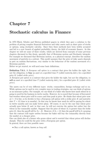
Vt = atSt + btβt = u(T − t, St), t ∈ [0, T] (7.12)
for some smooth deterministic function u(t, x). This is again another assumption, since we
assume that the value of our portfolio depends in a smooth way on t and St. We have the
following terminal condition
VT = u(0, ST ) = (ST − K)+
(7.13)
and this condition is necessary for arbitrage not to exist in our economy. For example, if VT =
u(0, ST ) < (ST −K)+
one could sell the portfolio for a value V0 and buy the option for a value V0
whose payoff is (ST −K)+
. The net profit would be in this case +V0 −V0 +(ST −K)+
−VT > 0.
The reverse strategy would be valid if VT = u(0, ST ) > (ST − K)+
.
Recall that St is a geometric Brownian motion, which in particular means that it satisfies the
following equation
Xt = X0 + µ
t
0
Xsds + σ
t
0
XsdBs (7.14)
so St is an Itˆo process with A(1)
= µX and A(2)
= σX. So we can apply the Itˆo formula from
theorem 6.6.1 to the process Vt = u(T − t, St). If we write f(t, x) = u(T − t, x) the partial
derivatives are
f1(t, x) = −u1(T − t, x), f2(t, x) = u2(T − t, x), f22(t, x) = u22(T − t, x) (7.15)
and the Itˆo formula yields
Vt − V0 =
t
0
[−u1(T − s, Ss) + µSsu2(T − s, Xs) +
1
2
σ2
S2
s u22(T − s, Xs)]ds (7.16)
+
t
0
[σSsu2(T − s, Xs)]dBs (7.17)
On the other hand, (at, bt) is self financing so
Vt − V0 =
t
0
asdSs +
s
0
bsdβs (7.18)
In order to be able to compare equations (7.17) and (7.18) we must first write (7.18) in the
same differentials as (7.17). Recall that
βt = β0ert
(7.19)
and thus
dβt = β0rert
dt = rβtdt (7.20)](https://image.slidesharecdn.com/edc87572-6bc2-40ac-a67c-f53bfedb3e6d-160930223103/85/tfg-72-320.jpg)
![CHAPTER 7. STOCHASTIC CALCULUS IN FINANCE 68
Moreover Vt = atSt + btβt so
bt =
Vt − atSt
βt
(7.21)
and combining this
bsdβs =
Vs − asSs
βs
rβsds (7.22)
We can also write dSs in terms of ds and dBs:
dSs = µSsds + σSsdBs (7.23)
Combining all this we can rewrite 7.18 as
Vt − V0 =
t
0
as(µSsds + σSsdBs) +
t
0
Vs − asSs
βs
rβsds (7.24)
=
t
0
[(µ − r)asSs + rVs]ds +
t
0
σasSsdBs (7.25)
Now we can compare identities 7.17 and 7.25. Because Vt is an Itˆo process its coefficients are
uniquely determined and thus
at = u2(T − t, St)
(µ − r)atSt + ru(T − t, St) = (µ − r)u2(T − t, St)St + ru(T − t, St)
= −u1(T − s, Ss) + µSsu2(T − s, Xs) +
1
2
σ2
S2
s u22(T − s, Xs)
and finally we can write from this last identity the following PDE
u1(t, x) =
1
2
σ2
x2
u22(t, x) + rxu2(t, x) − ru(t, x) (7.26)
for x > 0 and t ∈ [0, T] with the deterministic terminal condition u(0, x) = (x − K)+
. The
solution can be found explicitly. A full derivation can be found in section 14.5 in the book of
Rosario N. Mantegna [6].
Theorem 7.1.1 (Black-Scholes formula). The solution of the PDE 7.26 is
u(t, x) = xΦ(g(t, x)) − Ke−rt
Φ(h(t, x)) (7.27)
where
g(t, x) =
ln(x/K) + (r + 0.5σ2
)t
σt1/2
,
h(t, x) = g(t, x) − σt1/2
and
Φ(x) =
1
(2π)1/2
x
−∞
e−y2/2
dy, x ∈ R (7.28)
is the standard normal distribution.
Hence the rational price at time t = 0 for a European call option with strike price K is given
by
V0 = u(T, S0) = S0Φ(g(T, S0)) − KerT
Φ(h(T, S0)) (7.29)
Equation (7.29) is the celebrated Black-Scholes option pricing formula.](https://image.slidesharecdn.com/edc87572-6bc2-40ac-a67c-f53bfedb3e6d-160930223103/85/tfg-73-320.jpg)
![CHAPTER 7. STOCHASTIC CALCULUS IN FINANCE 69
Remark 7.1.1. The stochastic process Vt = u(T − t, St) is the value of the self-financing
portfolio at time t ∈ [0, T] and the self-financing strategy (at, bt) is given by
at = u2(T − t, St), bt =
u(T − t, St) − atSt
βt
(7.30)
Formula 7.29 is the most used formula for pricing options in finance. Part of its success comes
from the fact that it admits an explicit solution, which is quite rare when solving PDEs. Let’s
give an example of why is this formula so important.
Imagine that the price of the option at time t = 0 is p, with p = V0. Suppose that p > V0, then
one could do the following strategy:
ˆ Sell the option to someone else for a price of p. You gain p at t = 0
ˆ Invest V0 to buy a0 in stock and b0 in bonds, where a0 and b0 are given by (7.30). You
pay V0 at t = 0.
Following this strategy it is immediate to see that you obtain a net profit of p−V0 at t = 0. But
what’s interesting is that this profit remains unchanged at at maturity date T, no matter how
the stocks will move. Indeed, at T the value of our portfolio will be VT = u(0, ST ) = (ST −K)+
and we will have the obligation to pay (ST − K)+
to the buyer of our option. That means that
at T we will have had a cash flow equal to p − V0 + (ST − K)+
− (ST − K)+
for a net profit
of p − V0 > 0. We could increase the scale arbitrarily, selling n options for np and investing
nV0 in stocks and bonds for a net profit of n(p − V0), so we could obtain instantaneous and
unbounded profits.
Remark 7.1.2. Throughout the derivation we have implicitly or explicitly used a set of as-
sumptions. Let’s list them all here:
i) The stock price is an Itˆo process
ii) Security trading is continuous
iii) There are no arbitrage oportunities
iv) Selling of securities is possible at any time
v) There are no transaction costs
vi) The market interest rate r is constant
vii) There are no dividends between t = 0 and t = T
Provided that these assumptions hold, Black-Scholes formula gives the fair price of an option,
meaning that if an option is valued at a different price there exists an arbitrage opportunity.
7.1.2 Graphical representations of the Black-Scholes formula
We will see now some graphical representation for the price of an option. The following plots
have been obtained from the website [13]](https://image.slidesharecdn.com/edc87572-6bc2-40ac-a67c-f53bfedb3e6d-160930223103/85/tfg-74-320.jpg)
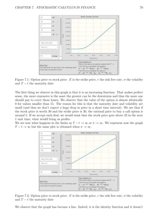

![Appendix A
Fokker-Planck equation
The Fokker–Planck equation is a partial differential equation that describes the time evolution
of the probability density function of the velocity of a particle under the influence of drag forces
and random forces. Let’s start with the evolution equation for a stochastic process x(t)
dx
dt
= q(x, t) + g(x, t)ξ(t) (A.1)
where q(x, t), g(x, t) are some deterministic functions and ξ(t) is white noise. So the process
has some deterministic function and has a random fluctuating component, described by g(x, t).
Because of this random component, one cannnot reach a deterministic solution. However, one
can instead define a function P(x, t) which gives us the probability that the solution x(t) of the
SDE at time t has the value x, averaged over all the possible realizations of the noise. One can
arrive to the formula
∂P(x, t)
∂t
= −
∂
∂x
[q(x, t)P(x, t)] +
D
2
∂
∂x
g(x(t), t)[g(x(t), t)P(x, t)] (A.2)
For a Brownian motion one has q(x, t) = 0 and g(x, t) =
√
2D, so the Fokker-Planck equation
reads
∂P
∂t
= D
∂2
P
∂x2
(A.3)
which is the diffusion equation.
73](https://image.slidesharecdn.com/edc87572-6bc2-40ac-a67c-f53bfedb3e6d-160930223103/85/tfg-78-320.jpg)
![Appendix B
Results and definitions in Probability
Theorem B.0.1 (Chebyshev inequality).
P(|X − EX|) ≥ ε) ≤
V (X)
ε2
(B.1)
B.1 Conditional expectation
Definition B.1.1. Let (Ω, F, P) be a probability space and G ⊂ F a σ-algebra. Let X be a
random variable with E(|X|) < ∞. We say that the random variable E(X|G) is the conditional
expectation of X given G if E(X|G) is G-measurable and
A
E(X|G)dP =
A
XdP ∀A ∈ G (B.2)
If X is a random variable F−measurable and G ⊂ F, then E[X|G] is a G−measurable ran-
dom variable and it is the best estimation of X that is G−measurable. The existance of the
conditional expectation can be shown using the Theorem of Radon-Nikodym. There are some
properties that we will use:
Property B.1.1. By definition, E(X) = E(E(X|G)) for G a σ−algebra
Property B.1.2. If X is F−measurable, E(XY ) < ∞ and E(Y ) < ∞ then
E(XY |G) = XE(Y |G) (B.3)
Property B.1.3. If X is independent of G and E(X) < ∞, then
E(X|G) = E(X) (B.4)
74](https://image.slidesharecdn.com/edc87572-6bc2-40ac-a67c-f53bfedb3e6d-160930223103/85/tfg-79-320.jpg)
![Bibliography
[1] Bardina, Xavier. Caminant a l’atzar tots els camins porten a Roma. Revista Electr`onica
de Divulgaci´o Matem`atica Editada por el Departament de Matem`atiques de la Universitat
Aut`onoma de Barcelona, 2008.
[2] Billingsley, Patrick. Convergence of Probability Measures. New York: Wiley, 1999.
[3] G´ora, Pawel F. The theory of Brownian Motion: A Hundred’s Year Anniversary. Marian
Smoluchowski Institute of Physics. Jagellonian University, Cracow, Poland.
[4] Ioannis Karatzas. Brownian Motion and Stochastic Calculus. New York: Springer, cop. 1991
[5] Jolis, Maria. Apuntes de Probabilidad. Universitat Aut`onoma de Barcelona.
[6] Mantegna, Rosario N. and Stanley, H. Eugene. An introduction to Econophysics. Correla-
tions and Complexity in Finance. Cambridge University Press.
[7] M´endez, Vicen¸c; Campos, Daniel and Bartumeus Frederic. Stochastic Foundations in Move-
ment Ecology. Springer.
[8] Mikosch, Thomas. Elementary Stochastic Calculus with Finance in view. World scientific.
[9] M¨orters, Peter and Peres, Yuval. Brownian motion. Cambridge University Press.
[10] Samaniego Vidal, Daniel. Moviment Browni`a. Project from the course ‘Tend`encies Actuals
de les Matm`atiques’.
[11] S. Lemons, Don. An Introduction to Stochastic Processes in Physics. The Johns Hopkins
University Press Baltimore and London.
[12] Toral, Ra´ul and Colet, Pere. Stochastic Numerical Methods: An Introduction for Students
and Scientists. Wiley-VCH.
[13] http://socr.ucla.edu/htmls/HTML5/econ apps/BlackScholesPlot/BlackScholesPlot.html
[14] https://en.wikipedia.org/wiki/Put option
[15] https://en.wikipedia.org/wiki/Call option
[16] http://introcs.cs.princeton.edu/java/15inout/RandomWalk.java.html
75](https://image.slidesharecdn.com/edc87572-6bc2-40ac-a67c-f53bfedb3e6d-160930223103/85/tfg-80-320.jpg)


