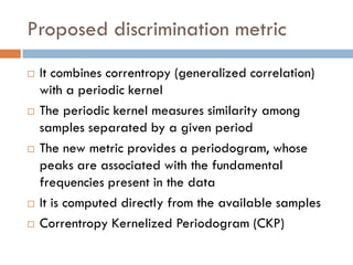
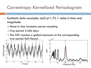
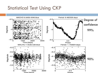
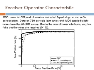
Download as PDF, PPTX

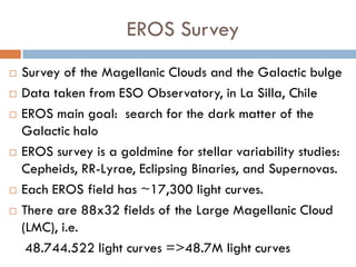
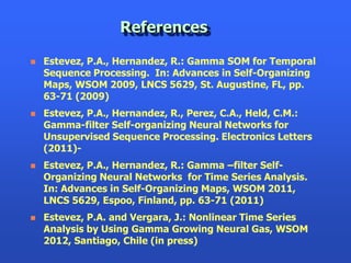
![Computational Time Requirements
for EROS Survey
Computational time measured using NVIDIA Tesla C2070
GPU (448 cores)
Sweeping 20000 trial periods with CKP, the total time
per light curve (~650 samples): 1.5 [s]
For 48.7M light curves: ~845 days!
Evaluating 600 precomputed trial periods (by using
correntropy and other methods) and optimizing the code:
0.2 [s] per light curve
For 48.7M million light curves: ~113 days!](https://image.slidesharecdn.com/pablo-121220153627-phpapp02/85/Pablo-Estevez-Computational-Intelligence-Applied-to-Time-Series-Analysis-13-320.jpg)


This document summarizes a presentation on analyzing astronomical time series data using information theoretic learning approaches. It discusses challenges with irregularly sampled and noisy light curve data from astronomical surveys. It proposes using correntropy, a generalized correlation measure, within a periodic kernel to create a Correntropy Kernelized Periodogram (CKP) for discriminating periodic vs non-periodic light curves and estimating periods of periodic curves. It applies this approach to real survey data from MACHO and EROS, achieving high classification accuracy and ability to process billions of light curves efficiently using GPU clusters.