Download as PDF, PPTX


![InstituteofComputingTechnology,ChineseAcademyofSciences
13
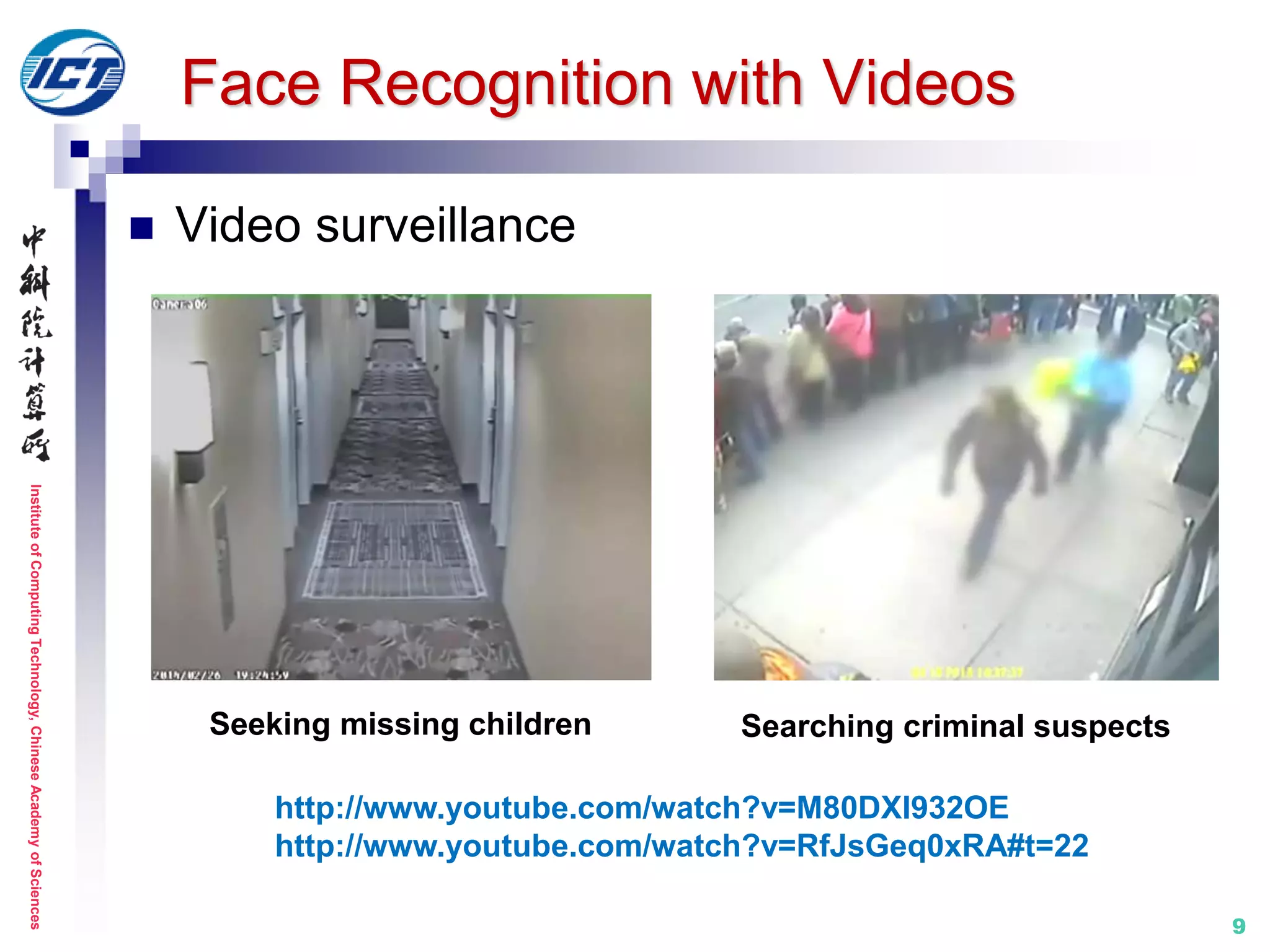
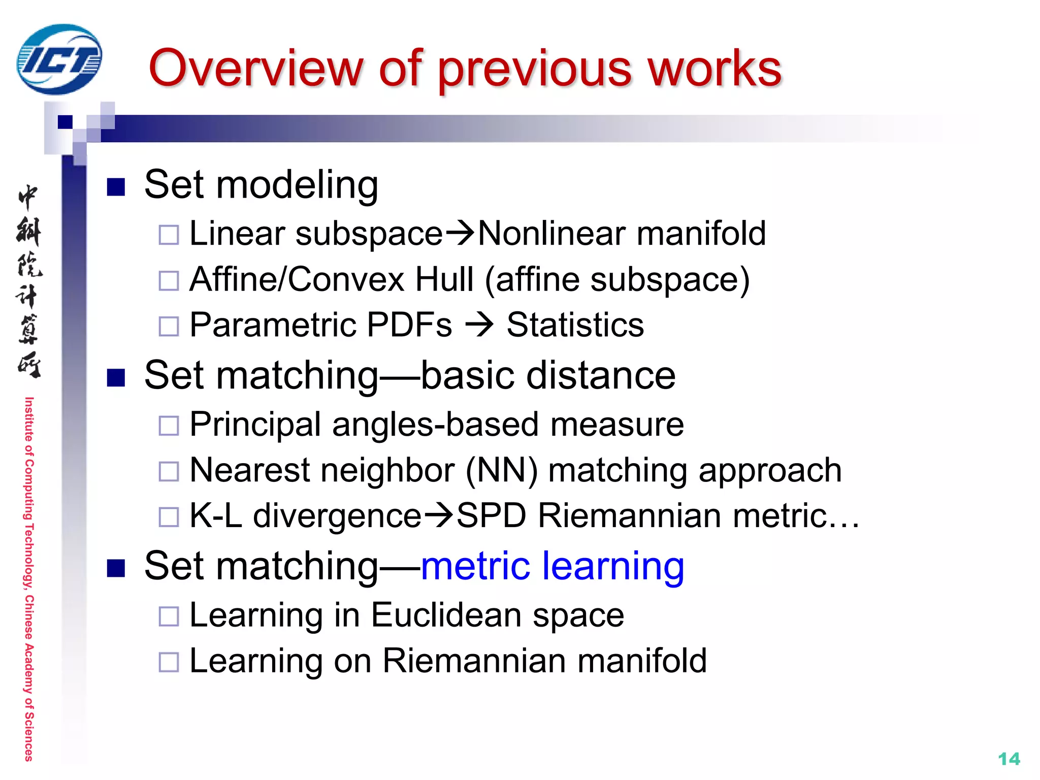
Overview of previous works
From the
view of set
modeling
Statistics
[Shakhnarovich, ECCV’02]
[Arandjelović, CVPR’05]
[Wang, CVPR’12]
[Harandi, ECCV’14]
[Wang, CVPR’15]
G1
G2
K-L
Divergence
S1
S2
Linear subspace
[Yamaguchi, FG’98]
[Kim, PAMI’07]
[Hamm, ICML’08]
[Huang, CVPR’15]
Principal
angle
H1
H2
Affine/Convex hull
[Cevikalp, CVPR’10]
[Hu, CVPR’11]
[Zhu, ICCV’13]
NN
matching
Nonlinear manifold
[Kim, BMVC’05]
[Wang, CVPR’08]
[Wang, CVPR’09]
[Chen, CVPR’13]
[Lu, CVPR’15]
Principal
angle(+)
M1
M2](https://image.slidesharecdn.com/0-report20150607cvprtutorialv3-150910074346-lva1-app6892/75/Distance-Metric-Learning-tutorial-at-CVPR-2015-13-2048.jpg)
![InstituteofComputingTechnology,ChineseAcademyofSciences
15
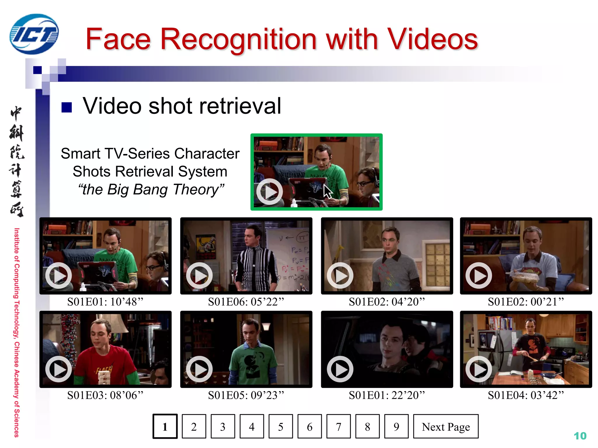
Set model I: linear subspace
Properties
PCA on the set of image samples to get subspace
Loose characterization of the set distribution region
Principal angles-based measure discards the
varying importance of different variance directions
Methods
MSM [FG’98]
DCC [PAMI’07]
GDA [ICML’08]
GGDA [CVPR’11]
PML [CVPR’15]
…
S1
S2
No distribution boundary
No direction difference](https://image.slidesharecdn.com/0-report20150607cvprtutorialv3-150910074346-lva1-app6892/75/Distance-Metric-Learning-tutorial-at-CVPR-2015-15-2048.jpg)
![InstituteofComputingTechnology,ChineseAcademyofSciences
16
Set model I: linear subspace
MSM (Mutual Subspace Method) [FG’98]
Pioneering work on image set classification
First exploit principal angles as subspace distance
Metric learning: N/A
[1] O. Yamaguchi, K. Fukui, and K. Maeda. Face Recognition Using Temporal Image
Sequence. IEEE FG 1998.
subspace method Mutual subspace method](https://image.slidesharecdn.com/0-report20150607cvprtutorialv3-150910074346-lva1-app6892/75/Distance-Metric-Learning-tutorial-at-CVPR-2015-16-2048.jpg)
![InstituteofComputingTechnology,ChineseAcademyofSciences
17
Set model I: linear subspace
DCC (Discriminant Canonical Correlations) [PAMI’07]
Metric learning: in Euclidean space
[1] T. Kim, J. Kittler, and R. Cipolla. Discriminative Learning and Recognition of Image
Set Classes Using Canonical Correlations. IEEE T-PAMI, 2007.
Set 1: 𝑿 𝟏 Set 2: 𝑿 𝟐
𝑷 𝟏
𝑷 𝟐
Linear subspace by:
orthonormal basis matrix
𝑿𝑖 𝑿𝑖
𝑇
≃ 𝑷𝑖 𝚲𝑖 𝑷𝑖
𝑇](https://image.slidesharecdn.com/0-report20150607cvprtutorialv3-150910074346-lva1-app6892/75/Distance-Metric-Learning-tutorial-at-CVPR-2015-17-2048.jpg)
![InstituteofComputingTechnology,ChineseAcademyofSciences
18
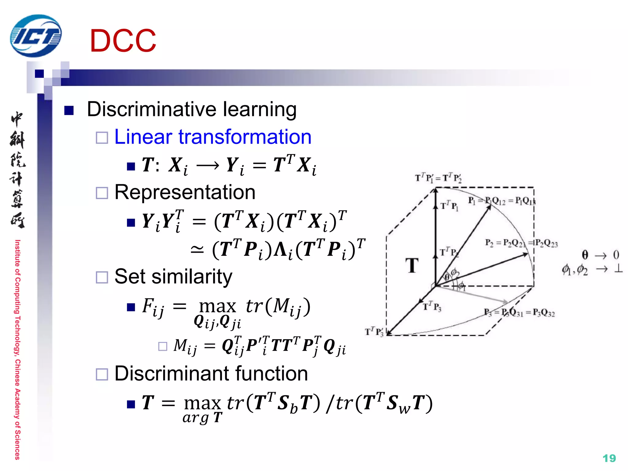
DCC
Canonical Correlations/Principal Angles
Canonical vectorscommon variation modes
Canonical vectors
Set 1: 𝑿 𝟏
Set 2: 𝑿 𝟐
𝑷1
𝑇
𝑷2 = 𝑸12 𝜦𝑸21
𝑇
𝑼 = 𝑷1 𝑸12 = [𝒖1, … , 𝒖2]
𝑽 = 𝑷2 𝑸21 = [𝒗1, … , 𝒗2]
𝜦 = 𝑑𝑖𝑎𝑔(cos 𝜃1, … , cos 𝜃 𝑑)
Canonical Correlation: cos 𝜃𝑖
Principal Angles: 𝜃𝑖
𝑷 𝟏
𝑷 𝟐](https://image.slidesharecdn.com/0-report20150607cvprtutorialv3-150910074346-lva1-app6892/75/Distance-Metric-Learning-tutorial-at-CVPR-2015-18-2048.jpg)
![InstituteofComputingTechnology,ChineseAcademyofSciences
20
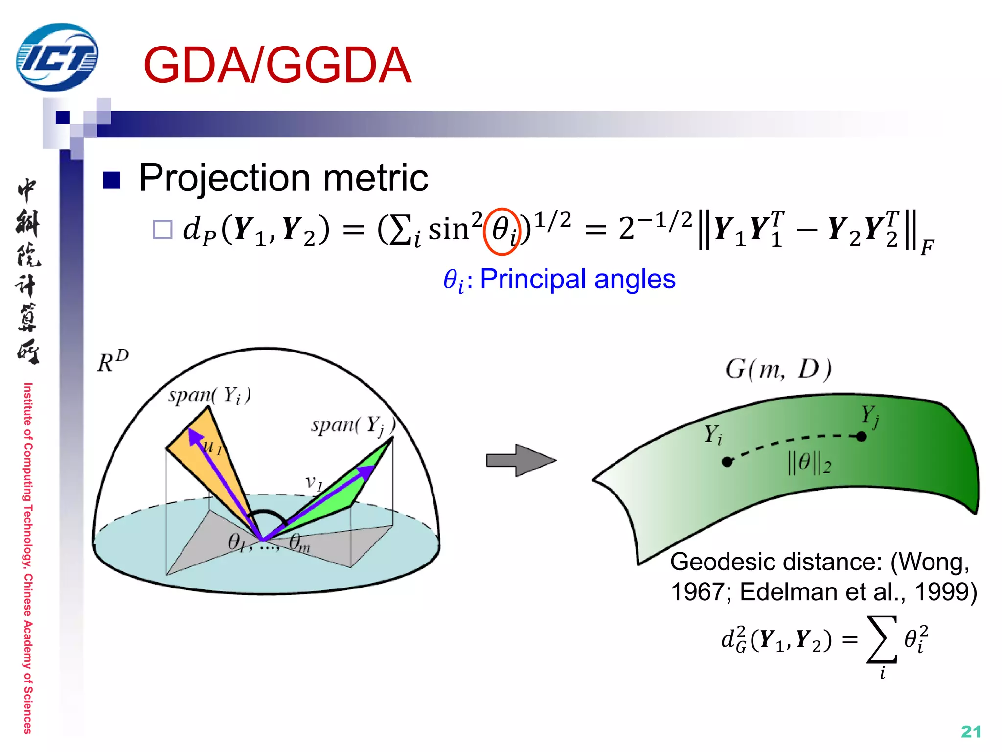
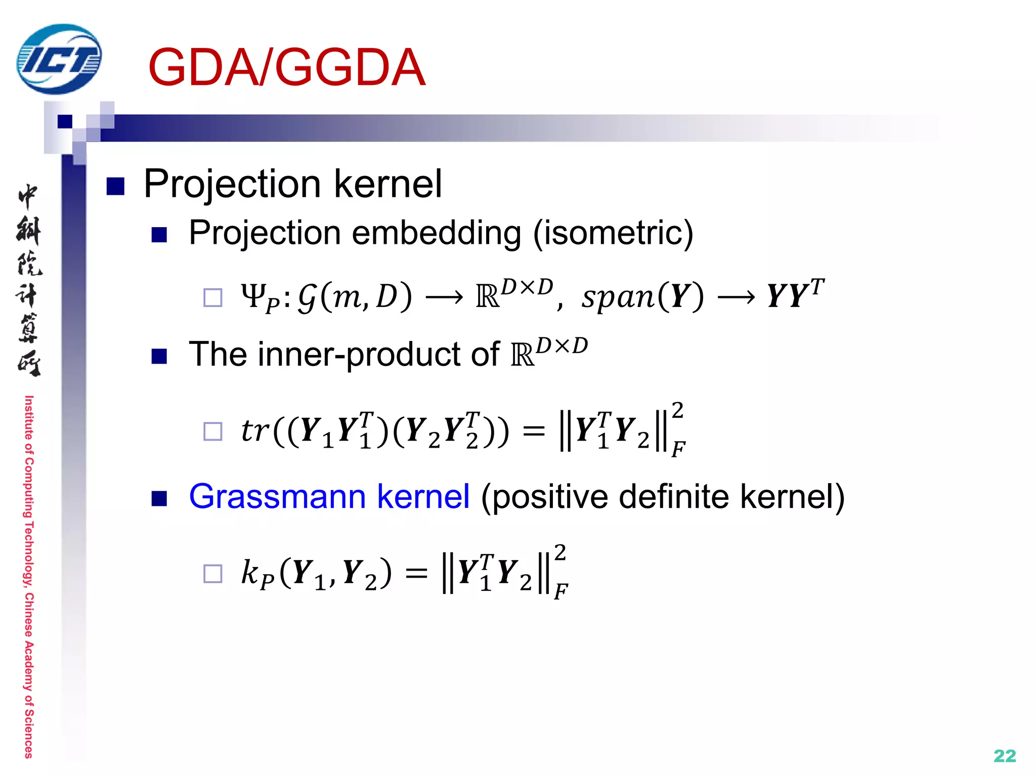
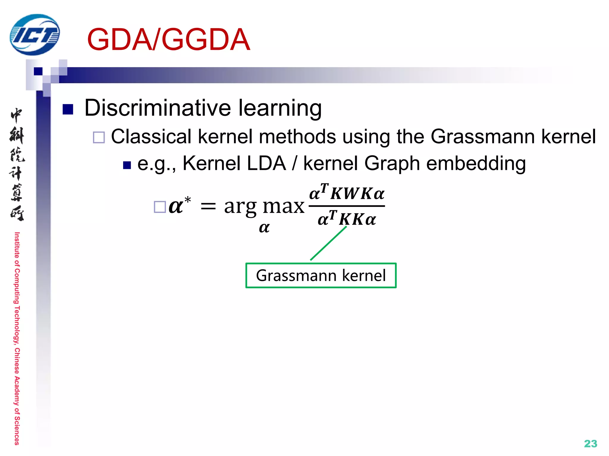
Set model I: linear subspace
GDA [ICML’08] / GGDA [CVPR’11]
Treat subspaces as points on Grassmann manifold
Metric learning: on Riemannian manifold
[1] J. Hamm and D. D. Lee. Grassmann Discriminant Analysis: a Unifying View on Subspace-Based
Learning. ICML 2008.
[2] M. Harandi, C. Sanderson, S. Shirazi, B. Lovell. Graph Embedding Discriminant Analysis on
Grassmannian Manifolds for Improved Image Set Matching. IEEE CVPR 2011.
Subspace Subspace
Grassmann manifold
implicit kernel
mapping](https://image.slidesharecdn.com/0-report20150607cvprtutorialv3-150910074346-lva1-app6892/75/Distance-Metric-Learning-tutorial-at-CVPR-2015-20-2048.jpg)
![InstituteofComputingTechnology,ChineseAcademyofSciences
24
Set model I: linear subspace
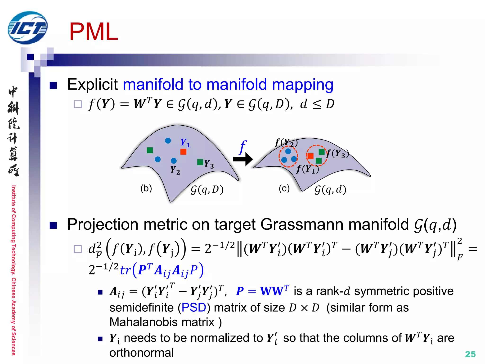
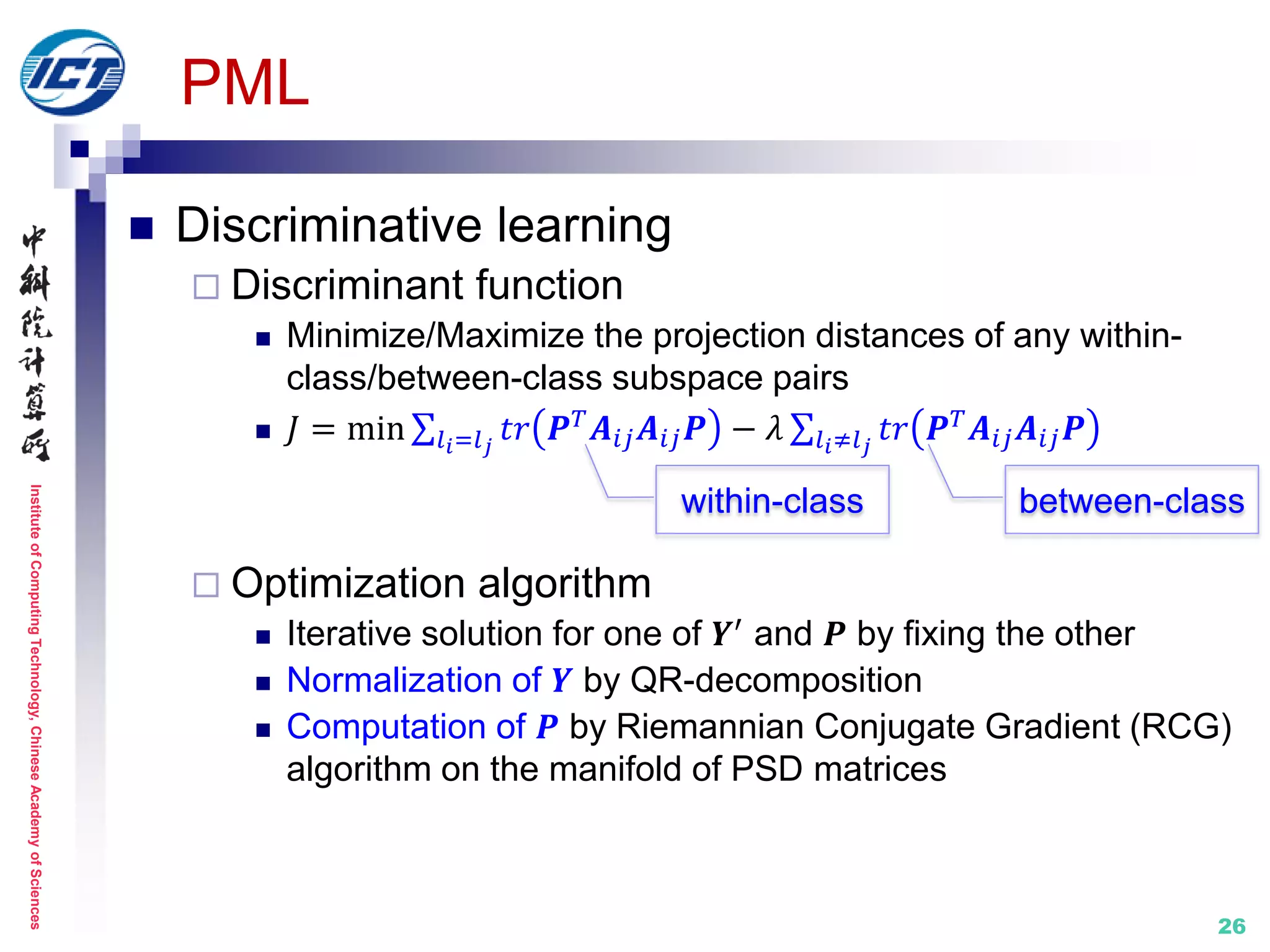
PML (Projection Metric Learning) [CVPR’15]
Metric learning: on Riemannian manifold
[1] Z. Huang, R. Wang, S. Shan, X. Chen. Projection Metric Learning on Grassmann Manifold with
Application to Video based Face Recognition. IEEE CVPR 2015.
(b) (c)(a)
𝒀1
𝒀 𝟐
𝒀 𝟑
𝒀 𝟑
𝒀 𝟐
𝒀1
𝒢(𝑞, 𝐷)
𝒀1
𝒀 𝟑
𝒀 𝟐
𝒢(𝑞, 𝑑)
(d)
𝒀1
𝒀 𝟑
𝒀 𝟐
ℋ (e)
𝒀 𝟑
𝒀1
𝒀 𝟐
ℝ 𝑑
Learning with kernel in RKHS
Learning directly on the manifold
Structure distortion
No explicit mapping
High complexity](https://image.slidesharecdn.com/0-report20150607cvprtutorialv3-150910074346-lva1-app6892/75/Distance-Metric-Learning-tutorial-at-CVPR-2015-24-2048.jpg)
![InstituteofComputingTechnology,ChineseAcademyofSciences
27
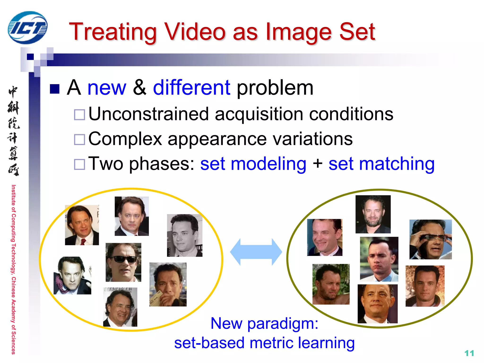
Set model II: nonlinear manifold
Properties
Capture nonlinear complex appearance variation
Need dense sampling and large amount of data
Less appealing computational efficiency
Methods
MMD [CVPR’08]
MDA [CVPR’09]
BoMPA [BMVC’05]
SANS [CVPR’13]
MMDML [CVPR’15]
…
Complex distribution
Large amount of data](https://image.slidesharecdn.com/0-report20150607cvprtutorialv3-150910074346-lva1-app6892/75/Distance-Metric-Learning-tutorial-at-CVPR-2015-27-2048.jpg)
![InstituteofComputingTechnology,ChineseAcademyofSciences
28
Set model II: nonlinear manifold
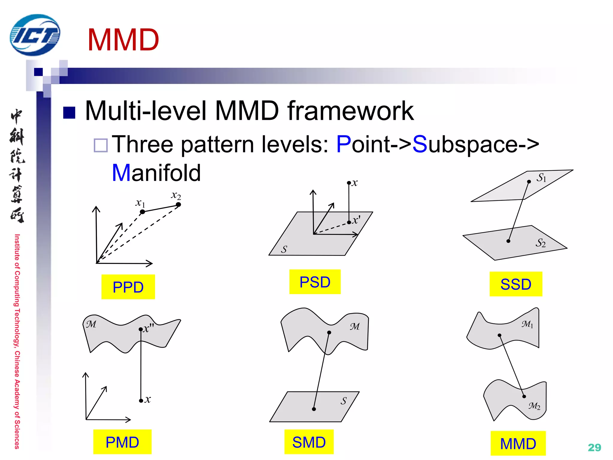
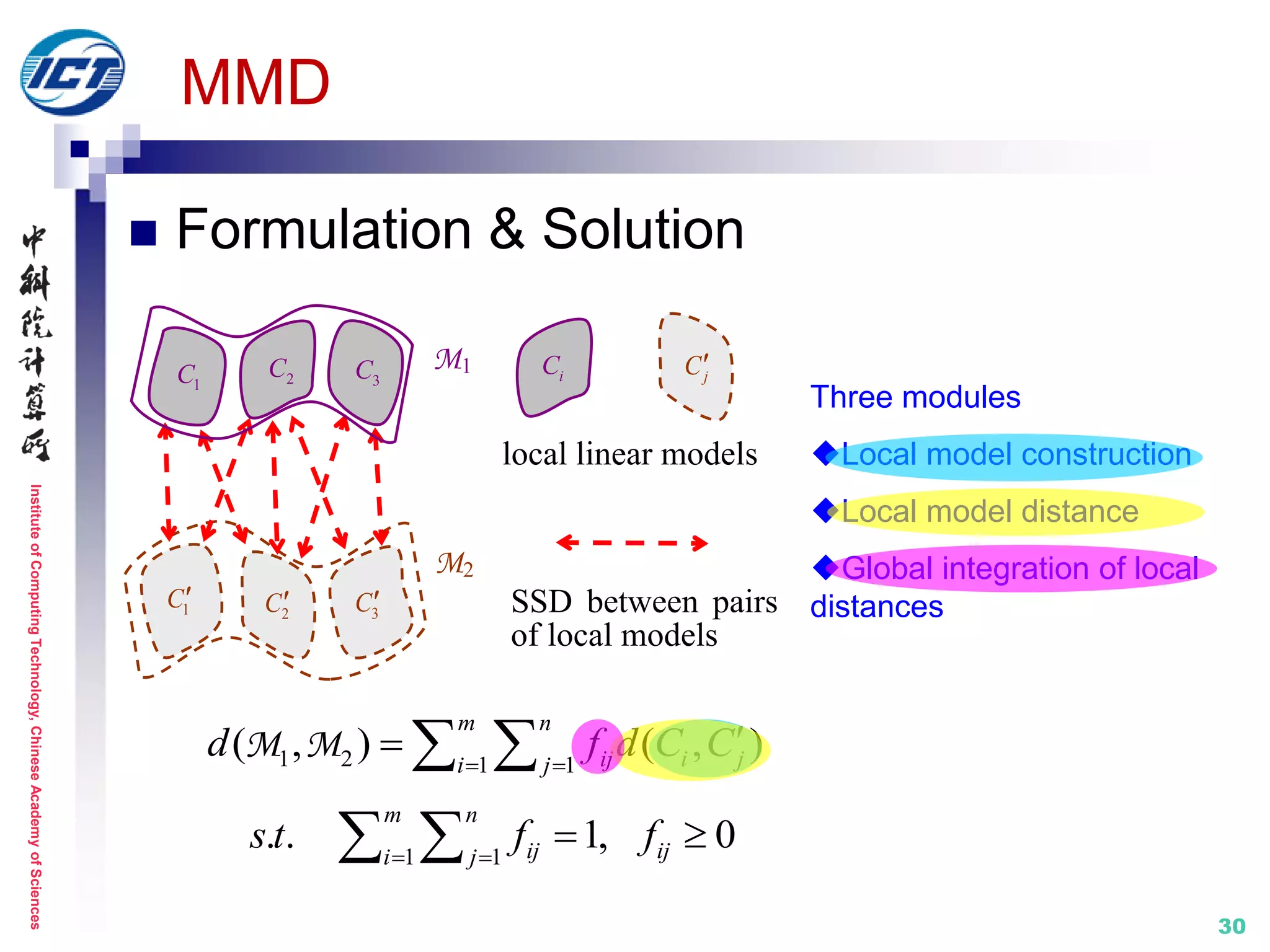
MMD (Manifold-Manifold Distance) [CVPR’08]
Set modeling with nonlinear appearance manifold
Image set classification distance computation
between two manifolds
Metric learning: N/A
D(M1,M2)
[1] R. Wang, S. Shan, X. Chen, W. Gao. Manifold-Manifold Distance with Application to Face
Recognition based on Image Set. IEEE CVPR 2008. (Best Student Poster Award Runner-up)
[2] R. Wang, S. Shan, X. Chen, Q. Dai, W. Gao. Manifold-Manifold Distance and Its Application to
Face Recognition with Image Sets. IEEE Trans. Image Processing, 2012.](https://image.slidesharecdn.com/0-report20150607cvprtutorialv3-150910074346-lva1-app6892/75/Distance-Metric-Learning-tutorial-at-CVPR-2015-28-2048.jpg)
![InstituteofComputingTechnology,ChineseAcademyofSciences
32
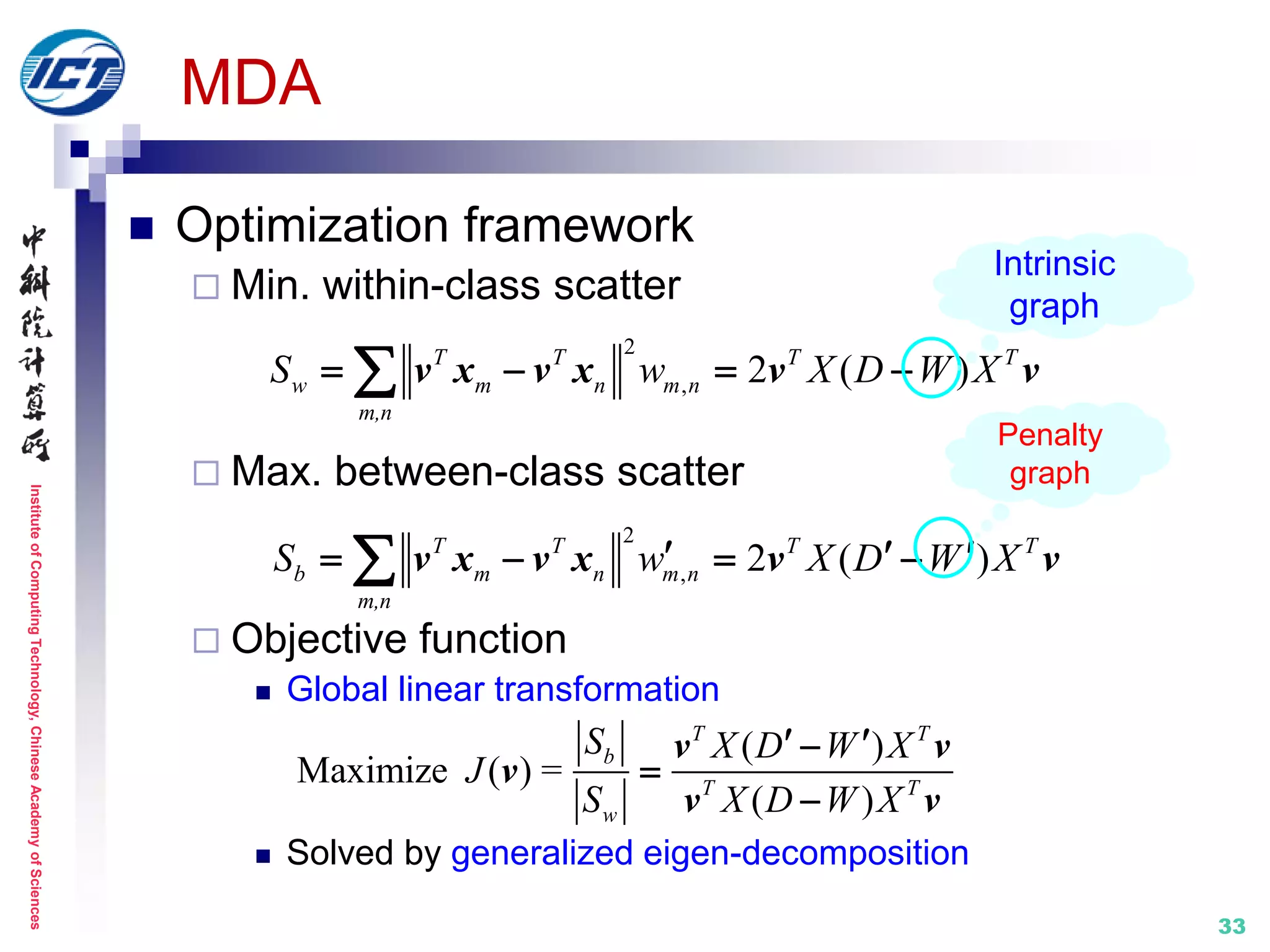
MDA (Manifold Discriminant Analysis ) [CVPR’09]
Goal: maximize “manifold margin” under Graph
Embedding framework
Metric learning: in Euclidean space
Euclidean distance between pair of image samples
[1] R. Wang, X. Chen. Manifold Discriminant Analysis. IEEE CVPR 2009.
M1
M2
within-class
compactness
between-class
separability
M1
M2
Intrinsic graph Penalty graph
Set model II: nonlinear manifold](https://image.slidesharecdn.com/0-report20150607cvprtutorialv3-150910074346-lva1-app6892/75/Distance-Metric-Learning-tutorial-at-CVPR-2015-32-2048.jpg)
![InstituteofComputingTechnology,ChineseAcademyofSciences
34
BoMPA (Boosted Manifold Principal Angles) [BMVC’05]
Goal: optimal fusion of different principal angles
Exploit Adaboost to learn weights for each angle
[1] T. Kim O. Arandjelovic, R. Cipolla. Learning over Sets using Boosted Manifold Principal Angles
(BoMPA). BMVC 2005.
PAsimilar (common illumination) BoMPAdissimilar
Subject A Subject B
Set model II: nonlinear manifold](https://image.slidesharecdn.com/0-report20150607cvprtutorialv3-150910074346-lva1-app6892/75/Distance-Metric-Learning-tutorial-at-CVPR-2015-34-2048.jpg)
![InstituteofComputingTechnology,ChineseAcademyofSciences
35
SANS (Sparse Approximated Nearest Subspaces) [CVPR’13]
Goal: adaptively construct the nearest subspace pair
Metric learning: N/A
[1] S. Chen, C. Sanderson, M.T. Harandi, B.C. Lovell. Improved Image Set Classification via Joint
Sparse Approximated Nearest Subspaces. IEEE CVPR 2013.
Set model II: nonlinear manifold
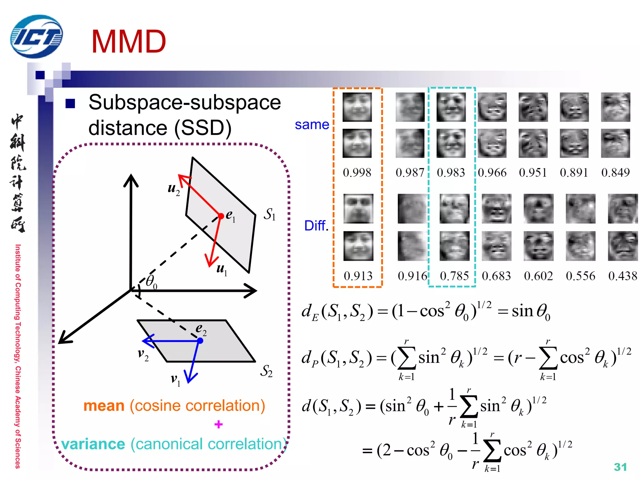
SSD (Subspace-Subspace Distance):
Joint sparse representation (JSR) is
applied to approximate the nearest
subspace over a Grassmann manifold.](https://image.slidesharecdn.com/0-report20150607cvprtutorialv3-150910074346-lva1-app6892/75/Distance-Metric-Learning-tutorial-at-CVPR-2015-35-2048.jpg)
![InstituteofComputingTechnology,ChineseAcademyofSciences
36
MMDML (Multi-Manifold Deep Metric Learning) [CVPR’15]
Goal: maximize “manifold margin” under Deep Learning
framework
Metric learning: in Euclidean space
Set model II: nonlinear manifold
[1] J. Lu, G. Wang, W. Deng, P. Moulin, and J. Zhou. Multi-Manifold Deep Metric Learning for Image
Set Classification. IEEE CVPR 2015.
Class-specific DNN
Model nonlinearity
Objective function](https://image.slidesharecdn.com/0-report20150607cvprtutorialv3-150910074346-lva1-app6892/75/Distance-Metric-Learning-tutorial-at-CVPR-2015-36-2048.jpg)
![InstituteofComputingTechnology,ChineseAcademyofSciences
37
Set model III: affine subspace
Properties
Linear reconstruction using: mean + subspace basis
Synthesized virtual NN-pair matching
Less characterization of global data structure
Computationally expensive by NN-based matching
Methods
AHISD/CHISD [CVPR’10]
SANP [CVPR’11]
PSDML/SSDML [ICCV’13]
…
H1
H2
Sensitive to noise samples
High computation cost](https://image.slidesharecdn.com/0-report20150607cvprtutorialv3-150910074346-lva1-app6892/75/Distance-Metric-Learning-tutorial-at-CVPR-2015-37-2048.jpg)
![InstituteofComputingTechnology,ChineseAcademyofSciences
38
Set model III: affine subspace
AHISD/CHISD [CVPR’10], SANP [CVPR’11]
NN-based matching using sample Euclidean distance
Metric learning: N/A
Subspace spanned by all the available samples
𝑫 = {𝑑1, … , 𝑑 𝑛} in the set
Affine hull
𝐻 𝑫 = 𝑫𝜶 = 𝑑𝑖 𝛼𝑖| 𝛼𝑖 = 1
Convex hull
𝐻 𝑫 = {𝑫𝜶 = 𝑑𝑖 𝛼𝑖| 𝛼𝑖 = 1, 0 ≤ 𝛼𝑖 ≤ 1}
[1] H. Cevikalp, B. Triggs. Face Recognition Based on Image Sets. IEEE CVPR 2010.
[2] Y. Hu, A.S. Mian, R. Owens. Sparse Approximated Nearest Points for Image Set
Classification. IEEE CVPR 2011.](https://image.slidesharecdn.com/0-report20150607cvprtutorialv3-150910074346-lva1-app6892/75/Distance-Metric-Learning-tutorial-at-CVPR-2015-38-2048.jpg)
![InstituteofComputingTechnology,ChineseAcademyofSciences
39
Set model III: affine subspace
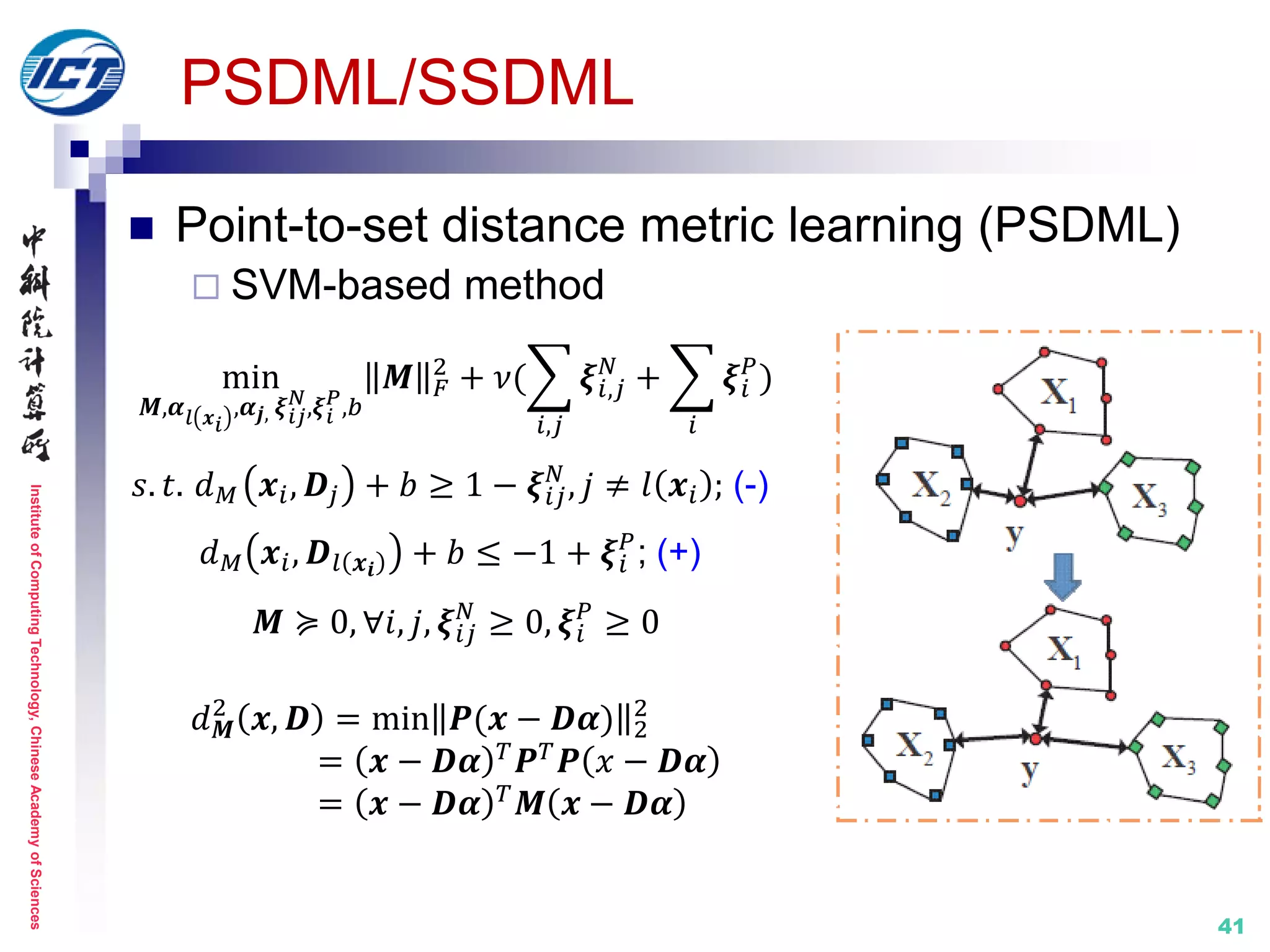
PSDML/SSDML [ICCV’13]
Metric learning: in Euclidean space
[1] P. Zhu, L. Zhang, W. Zuo, and D. Zhang. From Point to Set: Extend the Learning of
Distance Metrics. IEEE ICCV 2013.
point-to-set distance
metric learning (PSDML)
set-to-set distance metric
learning (SSDML)](https://image.slidesharecdn.com/0-report20150607cvprtutorialv3-150910074346-lva1-app6892/75/Distance-Metric-Learning-tutorial-at-CVPR-2015-39-2048.jpg)
![InstituteofComputingTechnology,ChineseAcademyofSciences
PSDML/SSDML
Set-to-set distance
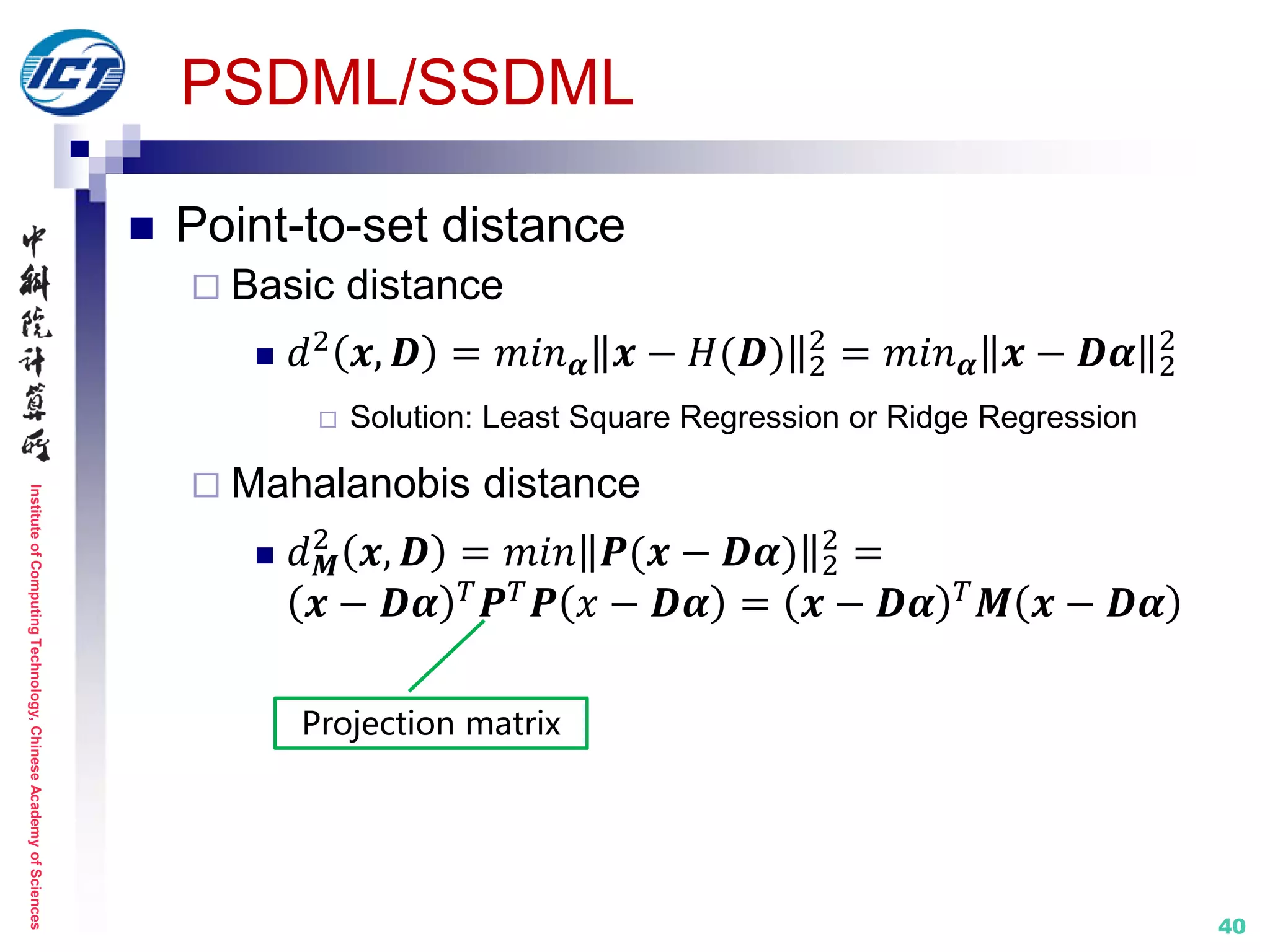
Basic distance
𝑑2 𝑫1, 𝑫2 = 𝑚𝑖𝑛 𝜶1,𝜶2
𝐻(𝑫1) − 𝐻(𝑫1) 2
2
=
𝑚𝑖𝑛 𝜶1,𝜶2
𝑫1 𝜶1 − 𝑫2 𝜶2 2
2
Solution: AHISD/CHISD [Cevikalp, CVPR’10]
Mahalanobis distance
𝑑 𝑴
2
𝑫1, 𝑫2 = 𝑚𝑖𝑛 𝑷(𝑫1 𝜶1 − 𝑫2 𝜶2) 2
2
=
𝑫1 𝜶1 − 𝑫2 𝜶2
𝑇 𝑴 𝑫1 𝜶1 − 𝑫2 𝜶2
42](https://image.slidesharecdn.com/0-report20150607cvprtutorialv3-150910074346-lva1-app6892/75/Distance-Metric-Learning-tutorial-at-CVPR-2015-42-2048.jpg)

![InstituteofComputingTechnology,ChineseAcademyofSciences
44
Set model IV: statistics (COV+)
Properties
The natural raw statistics of a sample set
Flexible model of multiple-order statistical information
Methods
CDL [CVPR’12]
LMKML [ICCV’13]
DARG [CVPR’15]
SPD-ML [ECCV’14]
LEML [ICML’15]
LERM [CVPR’14]
HER [CVPR’15 ]
…
G1
G2
Natural raw statistics
More flexible model
[Shakhnarovich, ECCV’02]
[Arandjelović, CVPR’05]](https://image.slidesharecdn.com/0-report20150607cvprtutorialv3-150910074346-lva1-app6892/75/Distance-Metric-Learning-tutorial-at-CVPR-2015-44-2048.jpg)
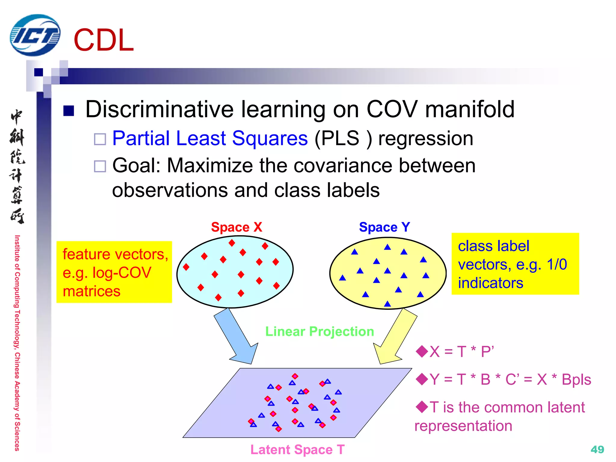
![InstituteofComputingTechnology,ChineseAcademyofSciences
45
CDL (Covariance Discriminative Learning) [CVPR’12]
Set modeling by Covariance Matrix (COV)
The 2nd order statistics characterizing set data variations
Robust to noisy set data, scalable to varying set size
Metric learning: on the SPD manifold
[1] R. Wang, H. Guo, L.S. Davis, Q. Dai. Covariance Discriminative Learning: A Natural
and Efficient Approach to Image Set Classification. IEEE CVPR 2012.
TI
log
Si
Ci Cj
Sj
I
Model data variations
No assum. of data distr.
Set model IV: statistics (COV+)](https://image.slidesharecdn.com/0-report20150607cvprtutorialv3-150910074346-lva1-app6892/75/Distance-Metric-Learning-tutorial-at-CVPR-2015-45-2048.jpg)
![InstituteofComputingTechnology,ChineseAcademyofSciences
46
CDL
Set modeling by Covariance Matrix
1 2= [ , ,..., ]N d NX x x x
COV: d*d symmetric positive
definite (SPD) matrix*
1
1
( )( )
1
N
T
i i
iN
C x x x x
Image set: N samples with d-
dimension image feature
*: use regularization to tackle singularity
problem](https://image.slidesharecdn.com/0-report20150607cvprtutorialv3-150910074346-lva1-app6892/75/Distance-Metric-Learning-tutorial-at-CVPR-2015-46-2048.jpg)
![InstituteofComputingTechnology,ChineseAcademyofSciences
47
CDL
Set matching on COV manifold
Riemannian metrics on the SPD manifold
Affine-invariant distance (AID) [1]
or
Log-Euclidean distance (LED) [2]
1 2 1 2( , ) log ( ) log ( ) F
d I IC C C C
2 2
1 2 1 21
( , ) ln ( , )
d
ii
d
C C C C
22 -1/2 -1/2
1 2 1 2 1( , ) log ( ) F
d IC C C C C
High
computational
burden
More efficient,
more appealing
[1] W. Förstner and B. Moonen. A Metric for Covariance Matrices. Technical Report 1999.
[2] V. Arsigny, P. Fillard, X. Pennec and N. Ayache. Geometric Means In A Novel Vector Space
Structure On Symmetric Positive-Definite Matrices. SIAM J. MATRIX ANAL. APPL. Vol. 29, No. 1, pp.
328-347, 2007.](https://image.slidesharecdn.com/0-report20150607cvprtutorialv3-150910074346-lva1-app6892/75/Distance-Metric-Learning-tutorial-at-CVPR-2015-47-2048.jpg)
![InstituteofComputingTechnology,ChineseAcademyofSciences
48
CDL
Set matching on COV manifold (cont.)
Explicit Riemannian kernel feature mapping with LED
1 2 1 2( , ) [log ( ) log ( )]logk trace I IC C C C
Mercer’s
theorem
Tangent space at
Identity matrix I
Riemannian manifold
of non-singular COV
M
TIM
X1 Y1
0
X2
X3
Y2
Y3
x1
x2
x3
y1
y2
y3
logI logI
: log ( ), ( )d d
log R
IC C](https://image.slidesharecdn.com/0-report20150607cvprtutorialv3-150910074346-lva1-app6892/75/Distance-Metric-Learning-tutorial-at-CVPR-2015-48-2048.jpg)
![InstituteofComputingTechnology,ChineseAcademyofSciences
COVSPD manifold
Model
Metric
Kernel
SubspaceGrassmannian
Model
Metric
Kernel
50
CDL vs. GDA
u1
u2
1
1
( )( )
1
N
T
i i
iN
C x x x x
*
T
C U U
1 2[ , , , ]m D mU u u u
1/ 2
1 2 1 1 2 2( , ) 2 T T
proj F
d
U U U U U U
: log ( ), ( )d d
log R
IC C : , ( , )T d d
proj m D R
U UU
1 2 1 2( , ) log ( ) log ( ) F
d I IC C C C
log ( ) log ( ) T
I IC U U](https://image.slidesharecdn.com/0-report20150607cvprtutorialv3-150910074346-lva1-app6892/75/Distance-Metric-Learning-tutorial-at-CVPR-2015-50-2048.jpg)
![InstituteofComputingTechnology,ChineseAcademyofSciences
51
LMKML (Localized Multi-Kernel Metric Learning) [ICCV’13]
Exploring multiple order statistics
Data-adaptive weights for different types of features
Ignoring the geometric structure of 2nd/3rd-order statistics
Metric learning: in Euclidean space
[1] J. Lu, G. Wang, and P. Moulin. Image Set Classification Using Holistic Multiple Order Statistics
Features and Localized Multi-Kernel Metric Learning. IEEE ICCV 2013.
Set model IV: statistics (COV+)
Complementary information
(mean vs. covariance)
1st / 2nd / 3rd-order statistics
Objective function](https://image.slidesharecdn.com/0-report20150607cvprtutorialv3-150910074346-lva1-app6892/75/Distance-Metric-Learning-tutorial-at-CVPR-2015-51-2048.jpg)
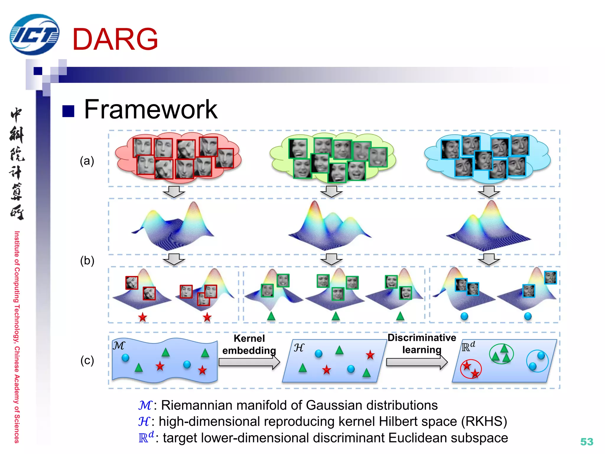
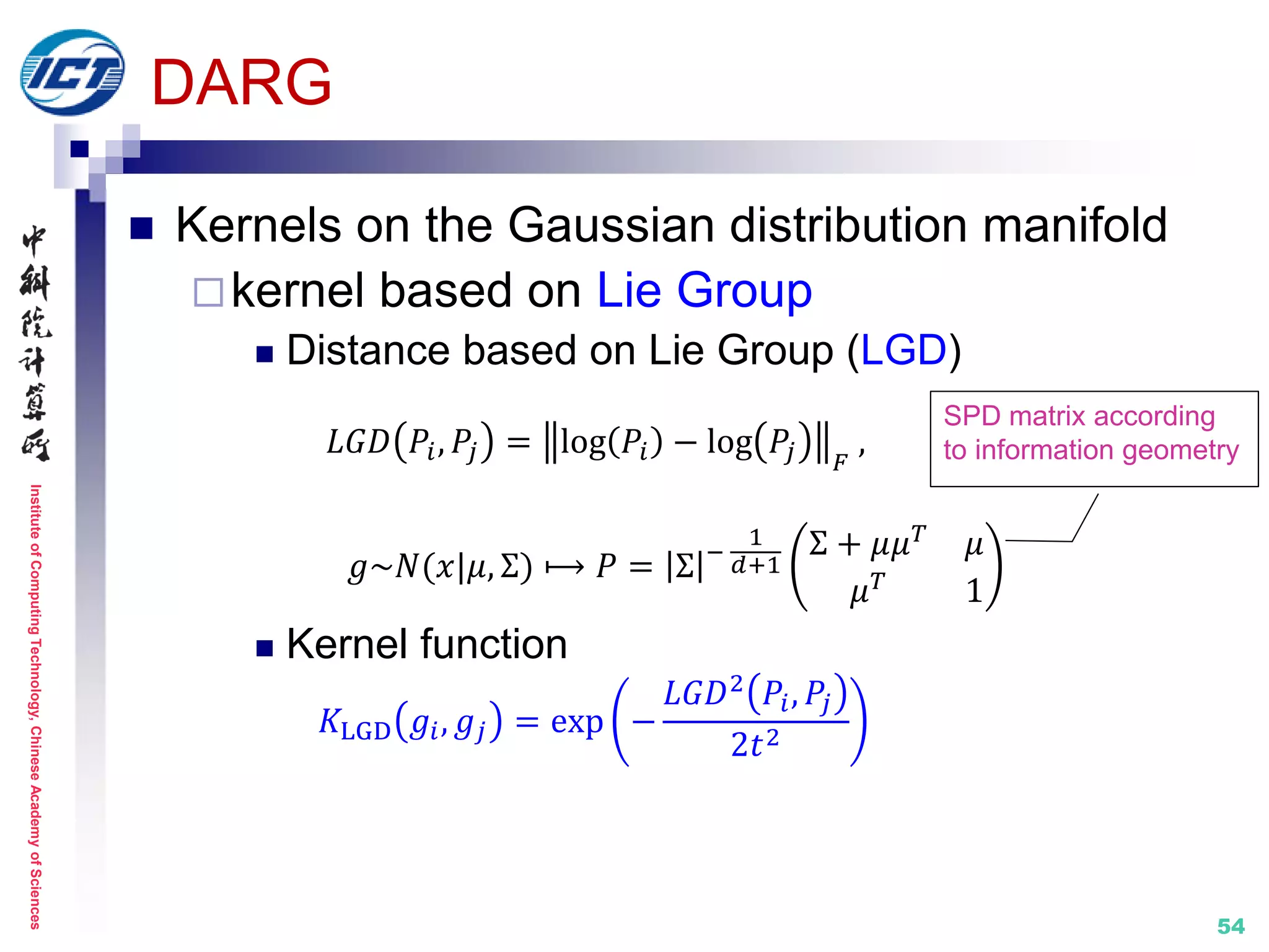
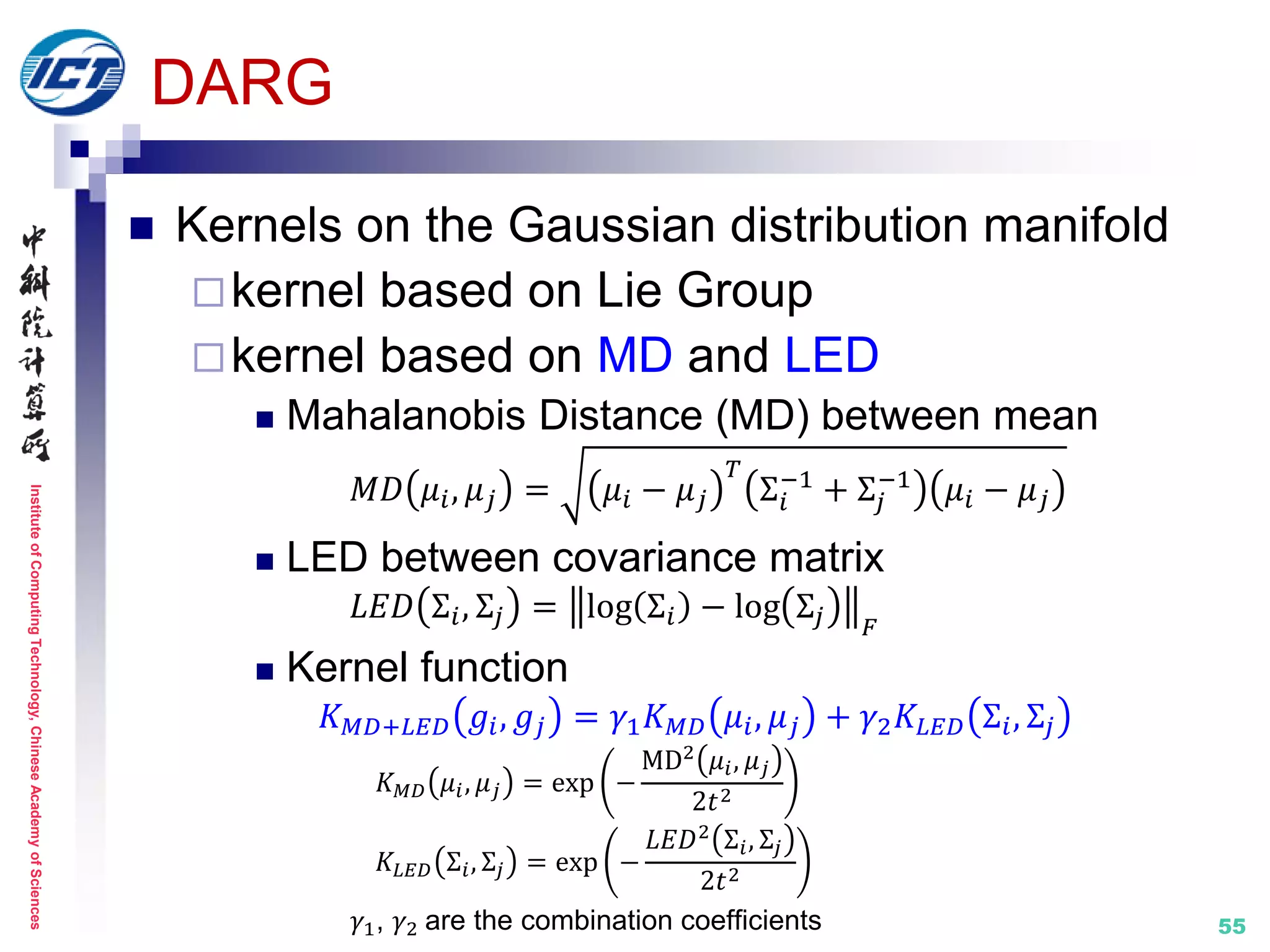
![InstituteofComputingTechnology,ChineseAcademyofSciences
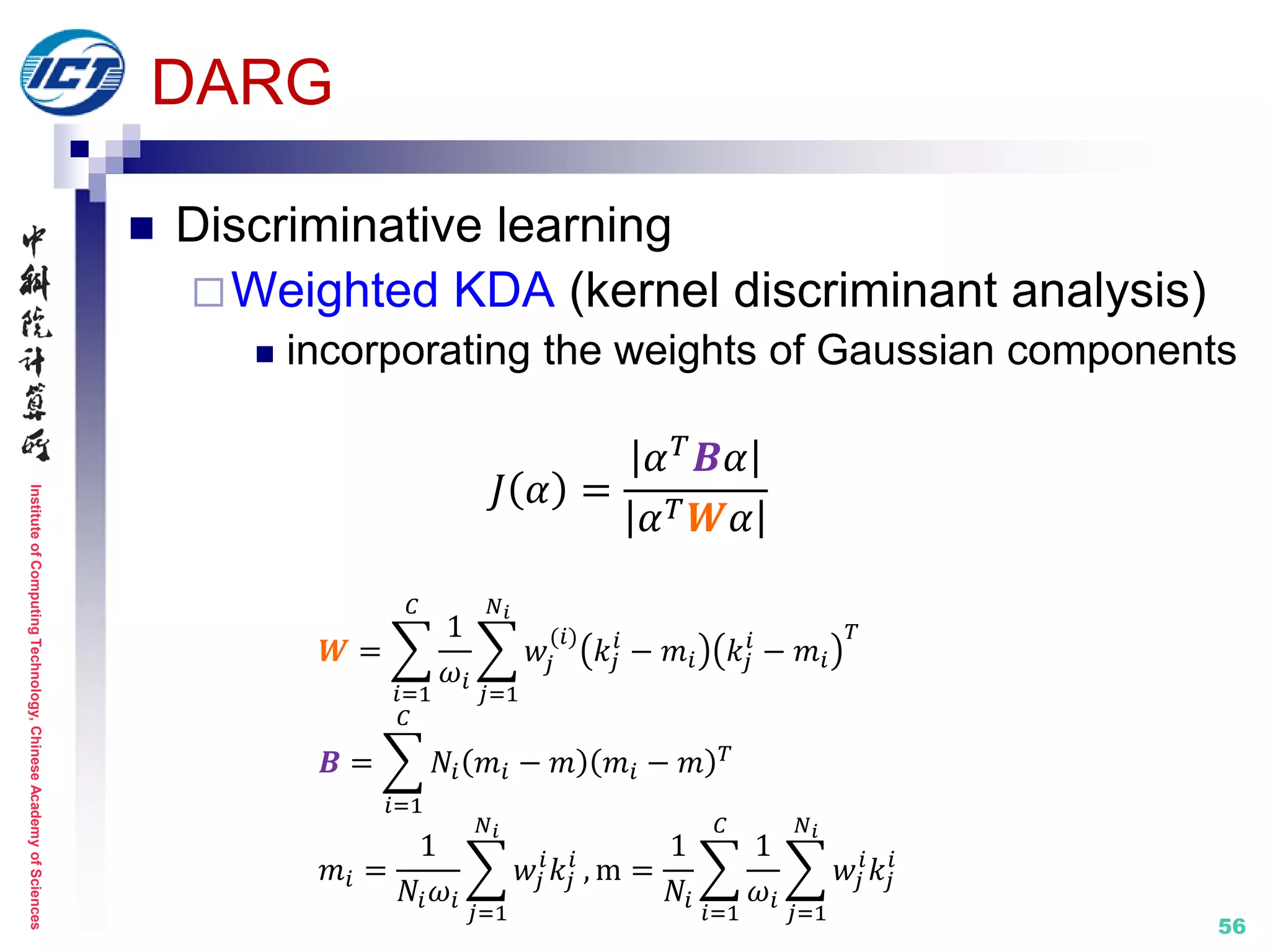
52
DARG (Discriminant Analysis on Riemannian manifold of
Gaussian distributions) [CVPR’15]
Set modeling by mixture of Gaussian distribution (GMM)
Naturally encode the 1st order and 2nd order statistics
Metric learning: on Riemannian manifold
[1] W. Wang, R. Wang, Z. Huang, S. Shan, X. Chen. Discriminant Analysis on Riemannian Manifold
of Gaussian Distributions for Face Recognition with Image Sets. IEEE CVPR 2015.
𝓜:Riemannian
manifold of Gaussian
distributions
Non-discriminative
Time-consuming
×
Set model IV: statistics (COV+)
[Shakhnarovich, ECCV’02]
[Arandjelović, CVPR’05]](https://image.slidesharecdn.com/0-report20150607cvprtutorialv3-150910074346-lva1-app6892/75/Distance-Metric-Learning-tutorial-at-CVPR-2015-52-2048.jpg)
![InstituteofComputingTechnology,ChineseAcademyofSciences
57
Set model IV: statistics (COV+)
Properties
The natural raw statistics of a sample set
Flexible model of multiple-order statistical information
Methods
CDL [CVPR’12]
LMKML [ICCV’13]
DARG [CVPR’15]
SPD-ML [ECCV’14]
LEML [ICML’15]
LERM [CVPR’14]
HER [CVPR’15 ]
…
G1
G2
Natural raw statistics
More flexible model
[Shakhnarovich, ECCV’02]
[Arandjelović, CVPR’05]](https://image.slidesharecdn.com/0-report20150607cvprtutorialv3-150910074346-lva1-app6892/75/Distance-Metric-Learning-tutorial-at-CVPR-2015-57-2048.jpg)
![InstituteofComputingTechnology,ChineseAcademyofSciences
58
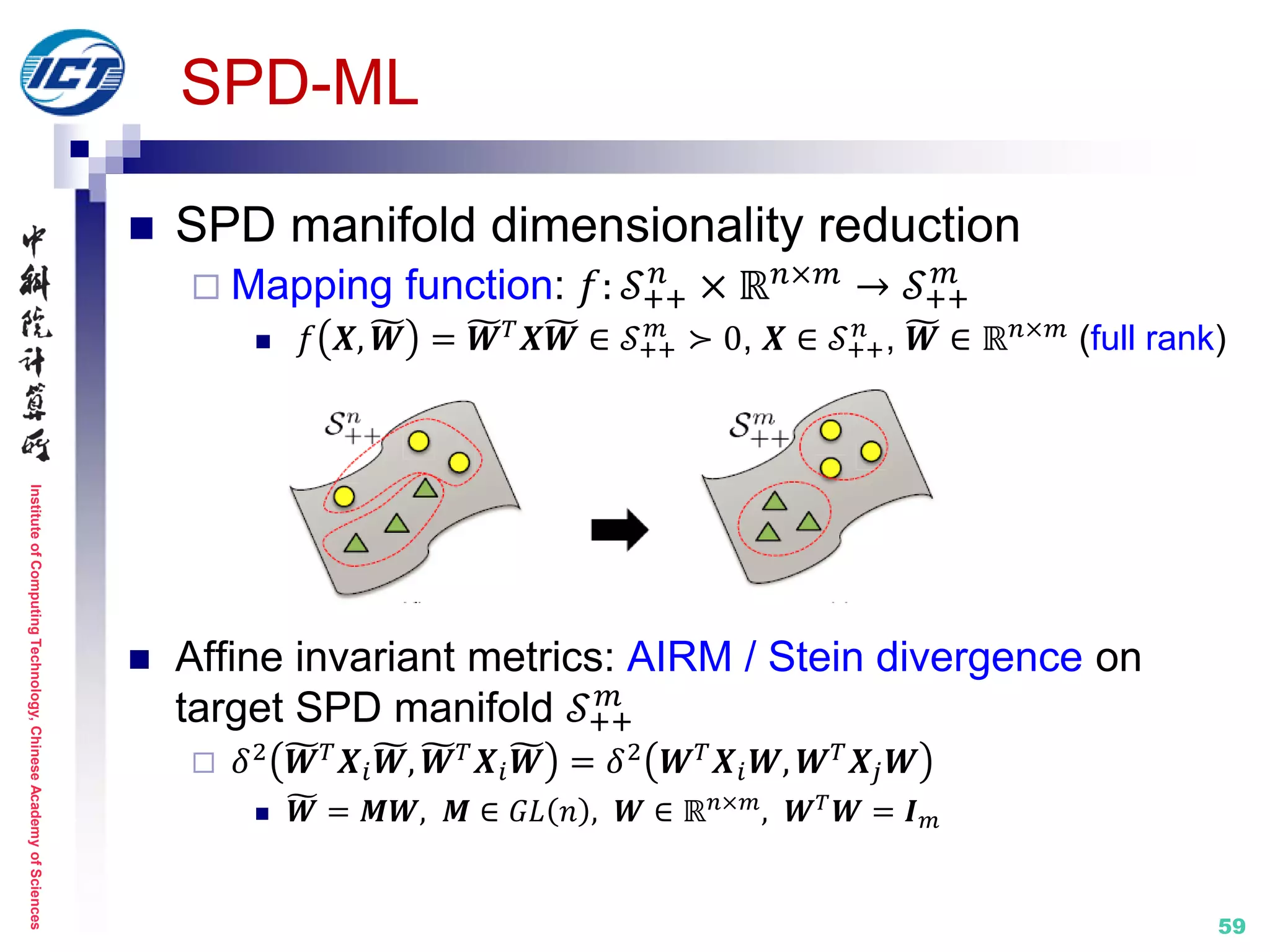
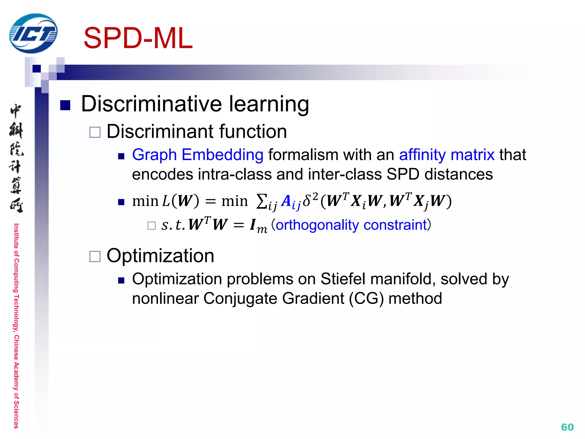
SPD-ML (SPD Manifold Learning) [ECCV’14]
Pioneering work on explicit manifold-to-manifold
dimensionality reduction
Metric learning: on Riemannian manifold
Set model IV: statistics (COV+)
[1] M. Harandi, M. Salzmann, R. Hartley. From Manifold to Manifold: Geometry-Aware
Dimensionality Reduction for SPD Matrices. ECCV 2014.
Structure distortion
No explicit mapping](https://image.slidesharecdn.com/0-report20150607cvprtutorialv3-150910074346-lva1-app6892/75/Distance-Metric-Learning-tutorial-at-CVPR-2015-58-2048.jpg)
![InstituteofComputingTechnology,ChineseAcademyofSciences
61
LEML (Log-Euclidean Metric Learning) [ICML’15]
Learning tangent map by preserving matrix symmetric
structure
Metric learning: on Riemannian manifold
Set model IV: statistics (COV+)
[1] Z. Huang, R. Wang, S. Shan, X. Li, X. Chen. Log-Euclidean Metric Learning on Symmetric
Positive Definite Manifold with Application to Image Set Classification. ICML 2015.
CDL [CVPR’12]
(a)
(b2)
(c)
OR
× 𝟐
× 𝟐
× 𝟐
(b1)
(d) (e)](https://image.slidesharecdn.com/0-report20150607cvprtutorialv3-150910074346-lva1-app6892/75/Distance-Metric-Learning-tutorial-at-CVPR-2015-61-2048.jpg)
![InstituteofComputingTechnology,ChineseAcademyofSciences
62
LEML
SPD tangent map learning
Mapping function:𝐷𝐹: 𝑓 log(𝑺) = 𝑾 𝑇log(𝑺)𝑾
𝑾 is column full rank
Log-Euclidean distance in the target tangent space
𝑑 𝐿𝐸𝐷 𝑓(𝑻𝑖), 𝑓(𝑻𝑗) = ||𝑾 𝑇 𝑻𝑖 𝑾 − 𝑾 𝑇 𝑻𝑗 𝑾|| 𝐹
= 𝑡𝑟(𝑸(𝑻𝑖 − 𝑻𝑗)(𝑻𝑖 − 𝑻𝑗))
𝑺
𝜉 𝑆
𝑇𝑺 𝕊+
𝑑 𝑇𝐹(𝑺) 𝕊+
𝑘
𝐷𝐹 𝑺 [𝜉 𝑆]
𝕊+
𝑑
𝕊+
𝑘
𝐹(𝑺)
𝐹
𝑫𝑭(𝑺)
𝛾(𝑡) 𝐹(𝛾 𝑡 )
analogy to 2DPCA
𝑸 = (𝑾𝑾 𝑇
)2
𝑻 = log(𝑺)](https://image.slidesharecdn.com/0-report20150607cvprtutorialv3-150910074346-lva1-app6892/75/Distance-Metric-Learning-tutorial-at-CVPR-2015-62-2048.jpg)
![InstituteofComputingTechnology,ChineseAcademyofSciences
63
LEML
Discriminative learning
Objective function
arg min
𝑄,𝜉
𝐷𝑙𝑑 𝑸, 𝑸 𝟎 + 𝜂𝐷𝑙𝑑 𝝃, 𝝃 𝟎
s. t. , tr 𝑸𝑨𝑖𝑗
𝑇
𝐀 𝑖𝑗 ≤ 𝜉 𝒄 𝑖,𝑗 , 𝑖, 𝑗 ∈ 𝑺
tr 𝑸𝑨𝑖𝑗
𝑇
𝐀 𝑖𝑗 ≥ 𝜉 𝒄 𝑖,𝑗 , (𝑖, 𝑗) ∈ 𝑫
𝐀 𝑖𝑗 = log 𝑪𝑖 − log (𝑪𝑗), 𝐷𝑙𝑑: LogDet divergence
Optimization
Cyclic Bregman projection algorithm [Bregman’1967]](https://image.slidesharecdn.com/0-report20150607cvprtutorialv3-150910074346-lva1-app6892/75/Distance-Metric-Learning-tutorial-at-CVPR-2015-63-2048.jpg)
![InstituteofComputingTechnology,ChineseAcademyofSciences
64
Set model IV: statistics (COV+)
Properties
The natural raw statistics of a sample set
Flexible model of multiple-order statistical information
Methods
CDL [CVPR’12]
LMKML [ICCV’13]
DARG [CVPR’15]
SPD-ML [ECCV’14]
LEML [ICML’15]
LERM [CVPR’14]
HER [CVPR’15 ]
…
G1
G2
Natural raw statistics
More flexible model
[Shakhnarovich, ECCV’02]
[Arandjelović, CVPR’05]](https://image.slidesharecdn.com/0-report20150607cvprtutorialv3-150910074346-lva1-app6892/75/Distance-Metric-Learning-tutorial-at-CVPR-2015-64-2048.jpg)
![InstituteofComputingTechnology,ChineseAcademyofSciences
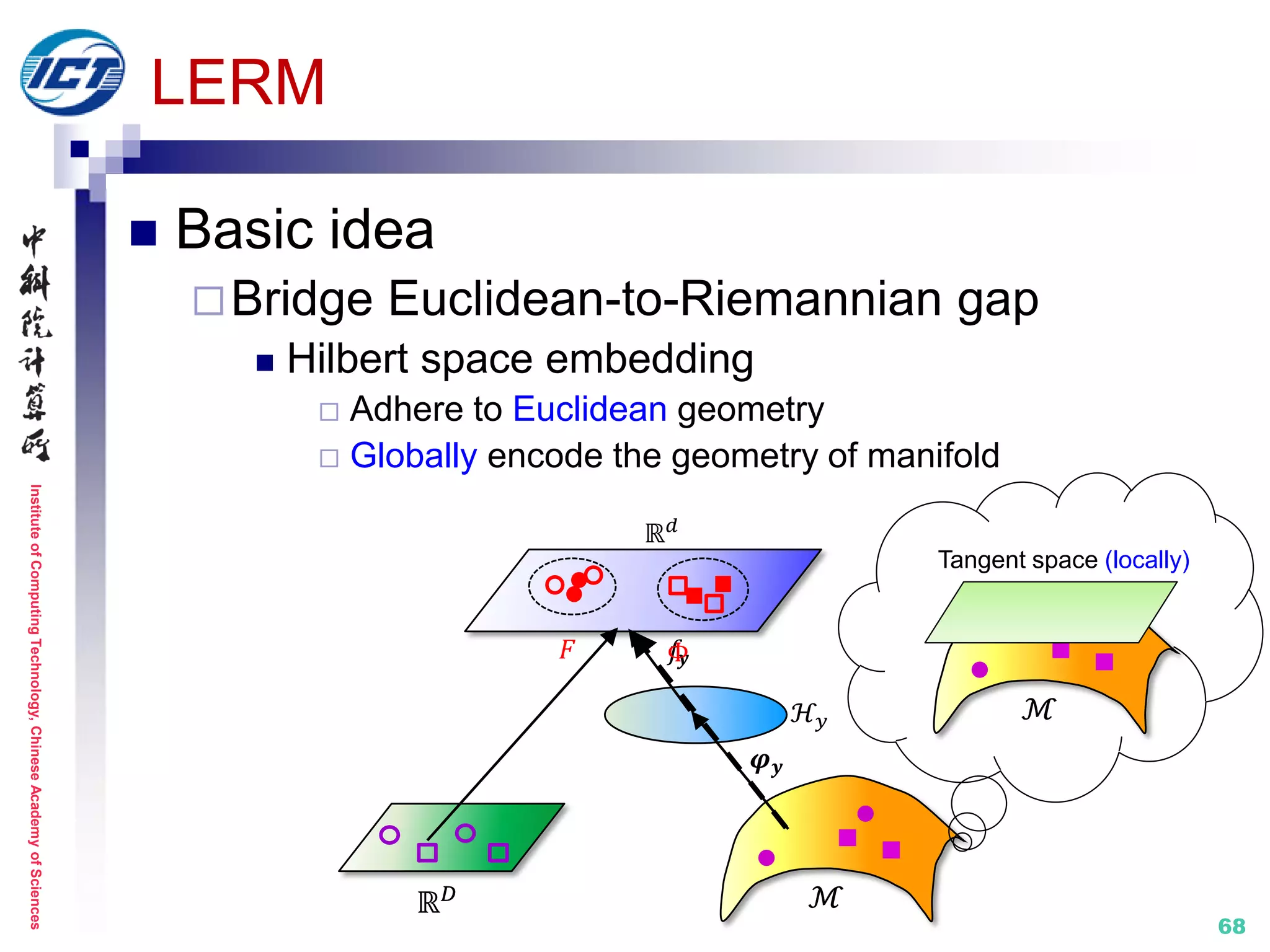
65
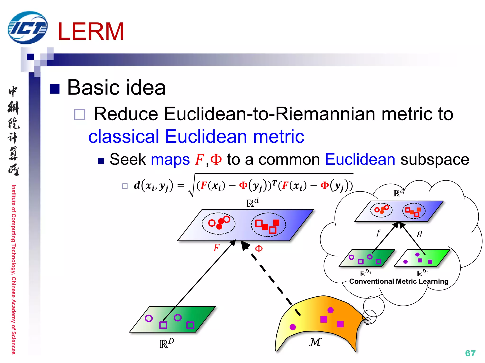
LERM (Learning Euclidean-to-Riemannian Metric) [CVPR’14]
Application scenario: still-to-video face recognition
Metric learning: cross Euclidean space and Riemannian manifold
[1] Z. Huang, R. Wang, S. Shan, X. Chen. Learning Euclidean-to-Riemannian Metric for Point-to-Set
Classification. IEEE CVPR 2014.
ℝ 𝐷
Watch list… Surveillance video
Point Set
Point-to-Set
Classification
Watch list screening
Set model IV: statistics (COV+)](https://image.slidesharecdn.com/0-report20150607cvprtutorialv3-150910074346-lva1-app6892/75/Distance-Metric-Learning-tutorial-at-CVPR-2015-65-2048.jpg)
![InstituteofComputingTechnology,ChineseAcademyofSciences
66
LERM
Point-to-Set Classification
Euclidean points vs. Riemannian points
ℳℝ 𝐷
[Hamm, ICML’08]
[Harandi, CVPR’11]
[Hamm, NIPS’08]
[Pennec, IJCV’06]
[Arsigny, SIAM’07]Point
Set model
Corresponding
manifold:
1.Grassmann (G)
2.AffineGrassmann (A)
3.SPD (S)
Euclidean space (E)
Heterogeneous
Linear subspace Affine hull Covariance matrixLinear subspace
[Yamaguchi, FG’98]
[Chien, PAMI’02]
[Kim, PAMI’07]
Affine hull
[Vincent, NIPS’01]
[Cevikalp, CVPR’10]
[Zhu, ICCV’13]
Covariance matrix
[Wang, CVPR’12]
[Vemulapalli, CVPR’13]
[Lu, ICCV’13]](https://image.slidesharecdn.com/0-report20150607cvprtutorialv3-150910074346-lva1-app6892/75/Distance-Metric-Learning-tutorial-at-CVPR-2015-66-2048.jpg)
![InstituteofComputingTechnology,ChineseAcademyofSciences
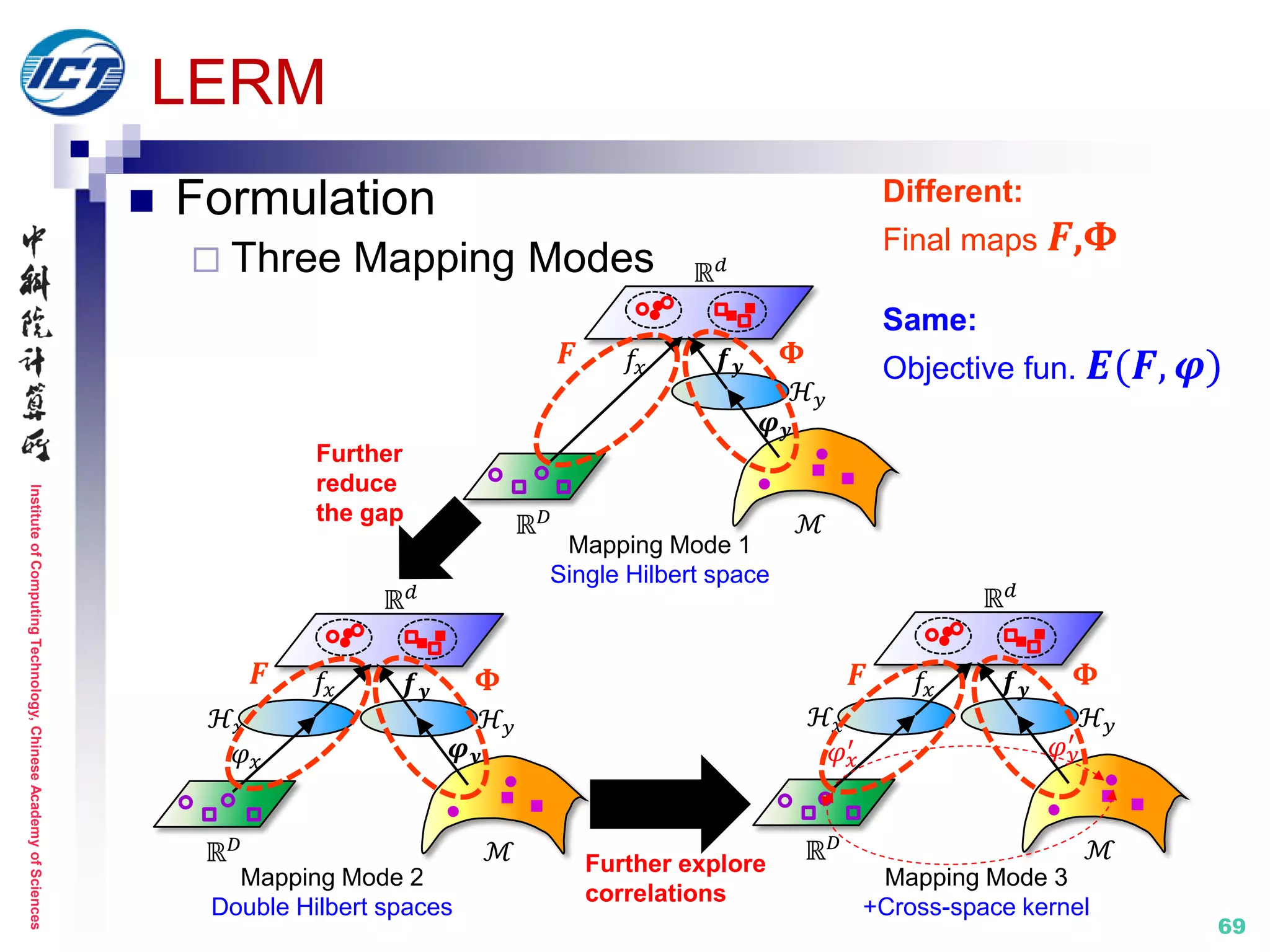
70
LERM
e.g. Mode 1
Further explore
correlations
ℝ 𝑑
ℋ𝑥
𝑓𝑥 𝒇 𝒚
ℝ 𝐷 ℳ
ℋ 𝑦
𝜑 𝑦
′
𝜑 𝑥
′
ℝ 𝑑
ℋ𝑥
𝑓𝑥 𝒇 𝒚
ℝ 𝐷 ℳ
ℋ 𝑦
𝜑 𝑦
′
𝜑 𝑥
′
Distance metric:
𝒅 𝒙𝒊, y𝒋 = (𝑭 𝒙𝒊 − 𝚽 𝒚𝒋 ) 𝑻(𝑭 𝒙𝒊 − 𝚽 𝒚𝒋 )
Objective function: 𝑬(𝑭, 𝝋)
min
𝐹,𝚽
{ 𝑫 𝑭, 𝚽 + 𝜆1 𝑮(𝑭, 𝚽) + 𝜆2 𝑻 𝑭, 𝚽 }
Distance Geometry Transformation
𝝋 𝒚
ℳ
ℋ 𝑦ℋ𝑥
𝜑 𝑥
ℝ 𝐷
ℝ 𝑑
𝒇 𝒚𝑓𝑥
Final maps:
𝑭 = 𝒇 𝒙 = 𝑾 𝒙
𝑻 𝑿
𝚽 = 𝒇 𝒚 ∘ 𝝋 𝒚 = 𝑾 𝒚
𝑻
𝑲 𝒚
𝝋 𝒚 𝒊
, 𝝋 𝒚 𝒋
= 𝐾 𝑦 𝑖, 𝑗
𝐾 𝑦 𝑖, 𝑗 = exp(−𝑑2(𝑦𝑖, 𝑦𝑗)/2𝜎2)
Single Hilbert space
Riemannian metrics [ICML’08, NIPS’08, SIAM’06]
ℝ 𝐷 ℳ
ℝ 𝑑
ℋ 𝑦
𝑓𝑥 𝒇 𝒚
𝝋 𝒚
Normalize Transformation
Discriminate Distance
Preserve Geometry
𝑭 𝚽](https://image.slidesharecdn.com/0-report20150607cvprtutorialv3-150910074346-lva1-app6892/75/Distance-Metric-Learning-tutorial-at-CVPR-2015-70-2048.jpg)
![InstituteofComputingTechnology,ChineseAcademyofSciences
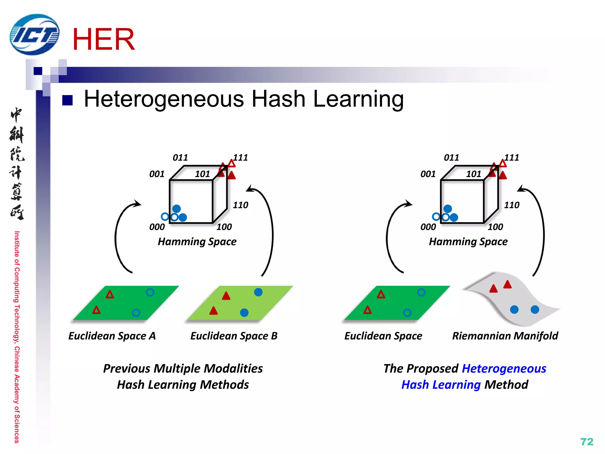
71
HER (Hashing across Euclidean and Riemannian) [CVPR’15]
Application scenario: video-based face retrieval
Metric learning: hamming distance learning across heter. spaces
[1] Y. Li, R. Wang, Z. Huang, S. Shan, X. Chen. Face Video Retrieval with Image Query via Hashing
across Euclidean Space and Riemannian Manifold. IEEE CVPR 2015.
Set model IV: statistics (COV+)](https://image.slidesharecdn.com/0-report20150607cvprtutorialv3-150910074346-lva1-app6892/75/Distance-Metric-Learning-tutorial-at-CVPR-2015-71-2048.jpg)
![InstituteofComputingTechnology,ChineseAcademyofSciences
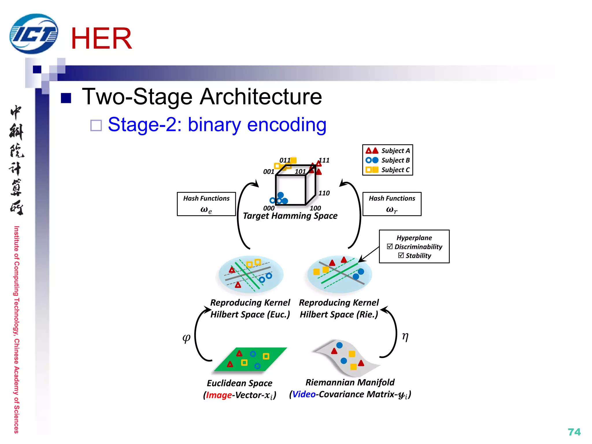
73
HER
Two-Stage Architecture
Stage-1: kernel mapping
Euclidean Kernel (Image)
𝑲 𝑒
𝑖𝑗
= exp(−
𝒙𝑖 − 𝒙𝑗 2
2
2𝜎𝑒
2 )
Riemannian Kernel (Video)
𝑲 𝑟
𝑖𝑗
= exp(−
log(𝔂𝑖) − log(𝔂 𝑗)
𝐹
2
2𝜎𝑟
2 )*
Reproducing Kernel
Hilbert Space (Euc.)
Reproducing Kernel
Hilbert Space (Rie.)
011
Target Hamming Space
001
111
110
100000
101
Subject A
Subject B
Subject C
𝜑 𝜂
[*] Y. Li, R. Wang, Z. Cui, S. Shan, X. Chen. Compact Video Code and Its Application to Robust Face
Retrieval in TV-Series. BMVC 2014. (**: CVC method for video-video face retrieval)
Euclidean Space
(Image-Vector-𝒙𝑖)
Riemannian Manifold
(Video-Covariance Matrix-𝔂𝑖)](https://image.slidesharecdn.com/0-report20150607cvprtutorialv3-150910074346-lva1-app6892/75/Distance-Metric-Learning-tutorial-at-CVPR-2015-73-2048.jpg)
![InstituteofComputingTechnology,ChineseAcademyofSciences
75
HER
Binary encoding [Rastegari, ECCV’12]
Discriminability
𝐸𝑒 = 𝑑(𝑩 𝑒
𝑚
, 𝑩 𝑒
𝑛
)
𝑚,𝑛∈𝑐𝑐∈{1:𝐶}
− 𝜆 𝑒 𝑑 𝑩 𝑒
𝑝
, 𝑩 𝑒
𝑞
𝑐2∈ 1:𝐶
𝑐1≠𝑐2,𝑞∈𝑐2
𝑐1∈ 1:𝐶
𝑝∈𝑐1
𝐸𝑟 = 𝑑(𝑩 𝑟
𝑚
, 𝑩 𝑟
𝑛
)
𝑚,𝑛∈𝑐𝑐∈{1:𝐶}
− 𝜆 𝑟 𝑑(𝑩 𝑟
𝑝
, 𝑩 𝑟
𝑞
)
𝑐2∈{1:𝐶}
𝑐1≠𝑐2,𝑞∈𝑐2
𝑐1∈{1:𝐶}
𝑝∈𝑐1
𝐸𝑒𝑟 = 𝑑(𝑩 𝑒
𝑚
, 𝑩 𝑟
𝑛
)
𝑚,𝑛∈𝑐𝑐∈{1:𝐶}
− 𝜆 𝑒𝑟 𝑑(𝑩 𝑒
𝑝
, 𝑩 𝑟
𝑞
)
𝑐2∈{1:𝐶}
𝑐1≠𝑐2,𝑞∈𝑐2
𝑐1∈{1:𝐶}
𝑝∈𝑐1
Objective Function
min
𝝎 𝑒,𝝎 𝑟,𝝃 𝑒,𝝃 𝑟,𝑩 𝑒,𝑩 𝑟
𝜆1 𝐸𝑒 + 𝜆2 𝐸𝑟 + 𝜆3 𝐸𝑒𝑟 + 𝛾1 𝝎 𝑒
𝑘 2
𝑘∈{1:𝐾}
+ 𝐶1 𝝃 𝑒
𝑘𝑖
𝑘∈{1:𝐾}
𝑖∈{1:𝑁}
+ 𝛾2 𝝎 𝑟
𝑘 2
𝑘∈{1:𝐾}
+ 𝐶2 𝝃 𝑟
𝑘𝑖
𝑘∈{1:𝐾}
𝑖∈{1:𝑁}
s.t.
𝑩 𝑒
𝑘𝑖
= 𝑠𝑔𝑛 𝝎 𝑒
𝑘 𝑇
𝜑 𝒙𝑖 , ∀𝑘 ∈ 1: 𝐾 , ∀𝑖 ∈ 1: 𝑁
𝑩 𝑟
𝑘𝑖
= 𝑠𝑔𝑛 𝝎 𝑟
𝑘 𝑇
𝜂 𝔂𝑖 , ∀𝑘 ∈ 1: 𝐾 , ∀𝑖 ∈ 1: 𝑁
𝑩 𝑟
𝑘𝑖
𝝎 𝑒
𝑘 𝑇
𝜑 𝒙𝑖 ≥ 1 − 𝝃 𝑒
𝑘𝑖
, 𝝃 𝑒
𝑘𝑖
> 0, ∀𝑘 ∈ 1: 𝐾 , ∀𝑖 ∈ 1: 𝑁
𝑩 𝑒
𝑘𝑖
𝝎 𝑟
𝑘 𝑇
𝜂 𝔂𝑖 ≥ 1 − 𝝃 𝑟
𝑘𝑖
, 𝝃 𝑟
𝑘𝑖
> 0, ∀𝑘 ∈ 1: 𝐾 , ∀𝑖 ∈ 1: 𝑁
Compatibility
(Cross-training)
Stability (SVM)
Discriminability (LDA)](https://image.slidesharecdn.com/0-report20150607cvprtutorialv3-150910074346-lva1-app6892/75/Distance-Metric-Learning-tutorial-at-CVPR-2015-75-2048.jpg)

![InstituteofComputingTechnology,ChineseAcademyofSciences
77
Evaluations
Two YouTube datasets
YouTube Celebrities (YTC) [Kim, CVPR’08]
47 subjects, 1910 videos from YouTube
YouTube FaceDB (YTF) [Wolf, CVPR’11]
3425 videos, 1595 different people
YTC
YTF](https://image.slidesharecdn.com/0-report20150607cvprtutorialv3-150910074346-lva1-app6892/75/Distance-Metric-Learning-tutorial-at-CVPR-2015-77-2048.jpg)
![InstituteofComputingTechnology,ChineseAcademyofSciences
78
Evaluations
COX Face [Huang, ACCV’12/TIP’15]
1,000 subjects
each has 1 high quality images, 3 unconstrained video
sequences
Images
Videos
http://vipl.ict.ac.cn/resources/datasets/cox-face-dataset/cox-face](https://image.slidesharecdn.com/0-report20150607cvprtutorialv3-150910074346-lva1-app6892/75/Distance-Metric-Learning-tutorial-at-CVPR-2015-78-2048.jpg)
![InstituteofComputingTechnology,ChineseAcademyofSciences
79
Evaluations
PaSC [Beveridge, BTAS’13]
Control videos
1 mounted video camera
1920*1080 resolution
Handheld videos
5 handheld video cameras
640*480~1280*720 resolution
Control video Handheld video](https://image.slidesharecdn.com/0-report20150607cvprtutorialv3-150910074346-lva1-app6892/75/Distance-Metric-Learning-tutorial-at-CVPR-2015-79-2048.jpg)
![InstituteofComputingTechnology,ChineseAcademyofSciences
80
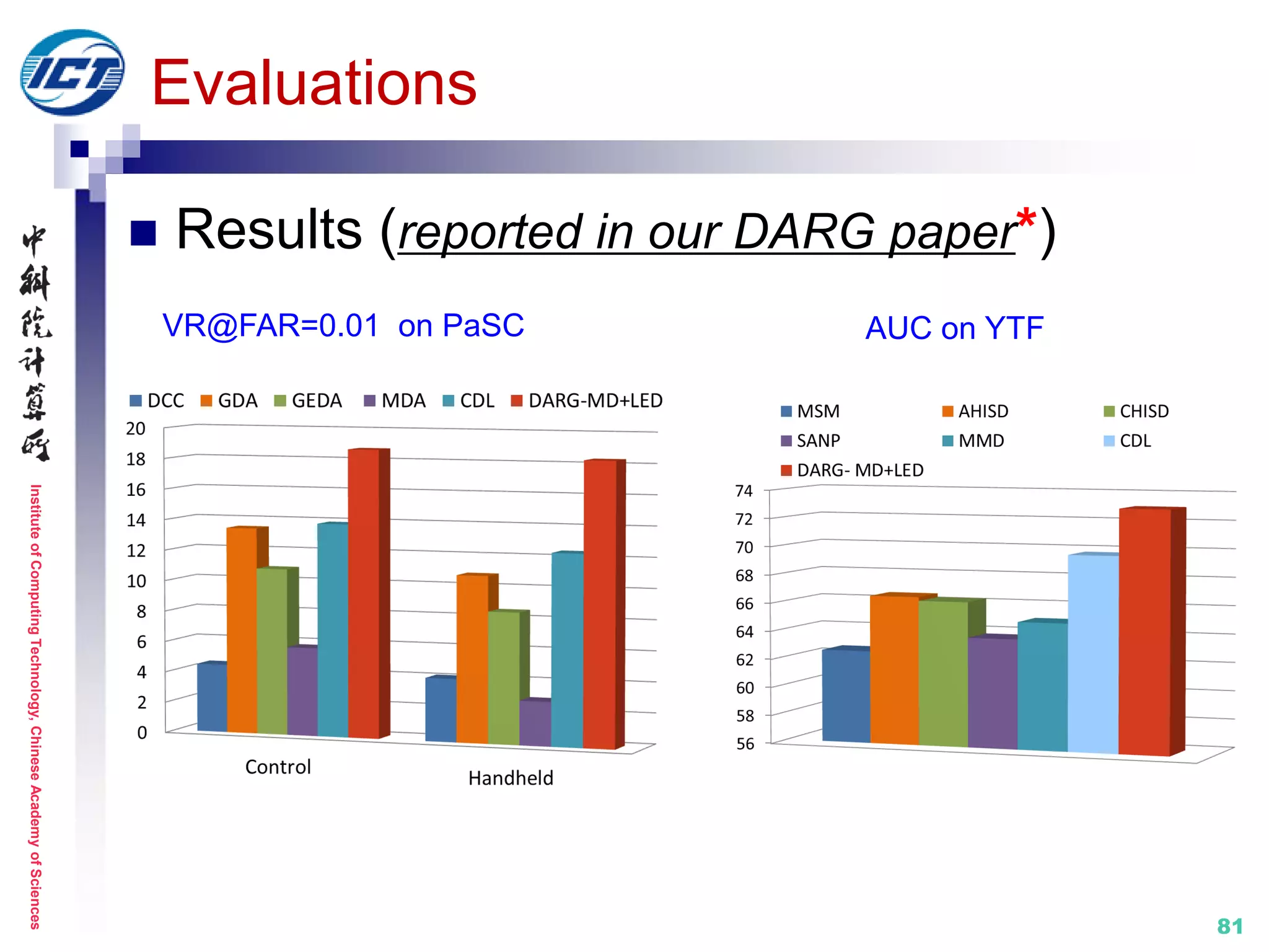
Evaluations
Results (reported in our DARG paper*)
[*] W. Wang, R. Wang, Z. Huang, S. Shan, X. Chen. Discriminant Analysis on Riemannian Manifold of
Gaussian Distributions for Face Recognition with Image Sets. IEEE CVPR 2015.](https://image.slidesharecdn.com/0-report20150607cvprtutorialv3-150910074346-lva1-app6892/75/Distance-Metric-Learning-tutorial-at-CVPR-2015-80-2048.jpg)
![InstituteofComputingTechnology,ChineseAcademyofSciences
82
Evaluations
Performance on PaSC Challenge (IEEE FG’15)
HERML-DeLF
DCNN learned image feature
Hybrid Euclidean and Riemannian Metric Learning*
[*] Z. Huang, R. Wang, S. Shan, X. Chen. Hybrid Euclidean-and-Riemannian Metric Learning for Image
Set Classification. ACCV 2014. (**: the key reference describing the method used for the challenge)](https://image.slidesharecdn.com/0-report20150607cvprtutorialv3-150910074346-lva1-app6892/75/Distance-Metric-Learning-tutorial-at-CVPR-2015-82-2048.jpg)
![InstituteofComputingTechnology,ChineseAcademyofSciences
83
Evaluations
Performance on EmotiW Challenge (ACM ICMI’14)*
Combination of multiple statistics for video modeling
Learning on the Riemannian manifold
[*] M. Liu, R. Wang, S. Li, S. Shan, Z. Huang, X. Chen. Combining Multiple Kernel Methods on
Riemannian Manifold for Emotion Recognition in the Wild. ACM ICMI 2014.](https://image.slidesharecdn.com/0-report20150607cvprtutorialv3-150910074346-lva1-app6892/75/Distance-Metric-Learning-tutorial-at-CVPR-2015-83-2048.jpg)

![InstituteofComputingTechnology,ChineseAcademyofSciences
87
Additional references (not listed above)
[Arandjelović, CVPR’05] O. Arandjelović, G. Shakhnarovich, J. Fisher, R.
Cipolla, and T. Darrell. Face Recognition with Image Sets Using Manifold
Density Divergence. IEEE CVPR 2005.
[Chien, PAMI’02] J. Chien and C. Wu. Discriminant waveletfaces and nearest
feature classifiers for face recognition. IEEE T-PAMI 2002.
[Rastegari, ECCV’12] M. Rastegari, A. Farhadi, and D. Forsyth. Attribute
discovery via predictable discriminative binary codes. ECCV 2012.
[Shakhnarovich, ECCV’02] G. Shakhnarovich, J. W. Fisher, and T. Darrell.
Face Recognition from Long-term Observations. ECCV 2002.
[Vemulapalli, CVPR’13] R. Vemulapalli, J. K. Pillai, and R. Chellappa. Kernel
learning for extrinsic classification of manifold features. IEEE CVPR 2013.
[Vincent, NIPS’01] P. Vincent and Y. Bengio. K-local hyperplane and convex
distance nearest neighbor algorithms. NIPS 2001.](https://image.slidesharecdn.com/0-report20150607cvprtutorialv3-150910074346-lva1-app6892/75/Distance-Metric-Learning-tutorial-at-CVPR-2015-87-2048.jpg)

This document summarizes Ruiping Wang's tutorial on distance metric learning for visual recognition. It provides an overview of previous works on set-based visual recognition, including set modeling approaches such as linear subspace, affine/convex hull, and nonlinear manifold models. It also reviews previous metric learning methods for set matching, including learning in Euclidean space and on Riemannian manifolds. Specific approaches discussed include mutual subspace method (MSM), discriminant canonical correlations (DCC), Grassmann discriminant analysis (GDA), and projection metric learning (PML).


![[DL輪読会]Recent Advances in Autoencoder-Based Representation Learning](https://cdn.slidesharecdn.com/ss_thumbnails/20190119dljournalclubweb-190401063633-thumbnail.jpg?width=640&height=640&fit=bounds)