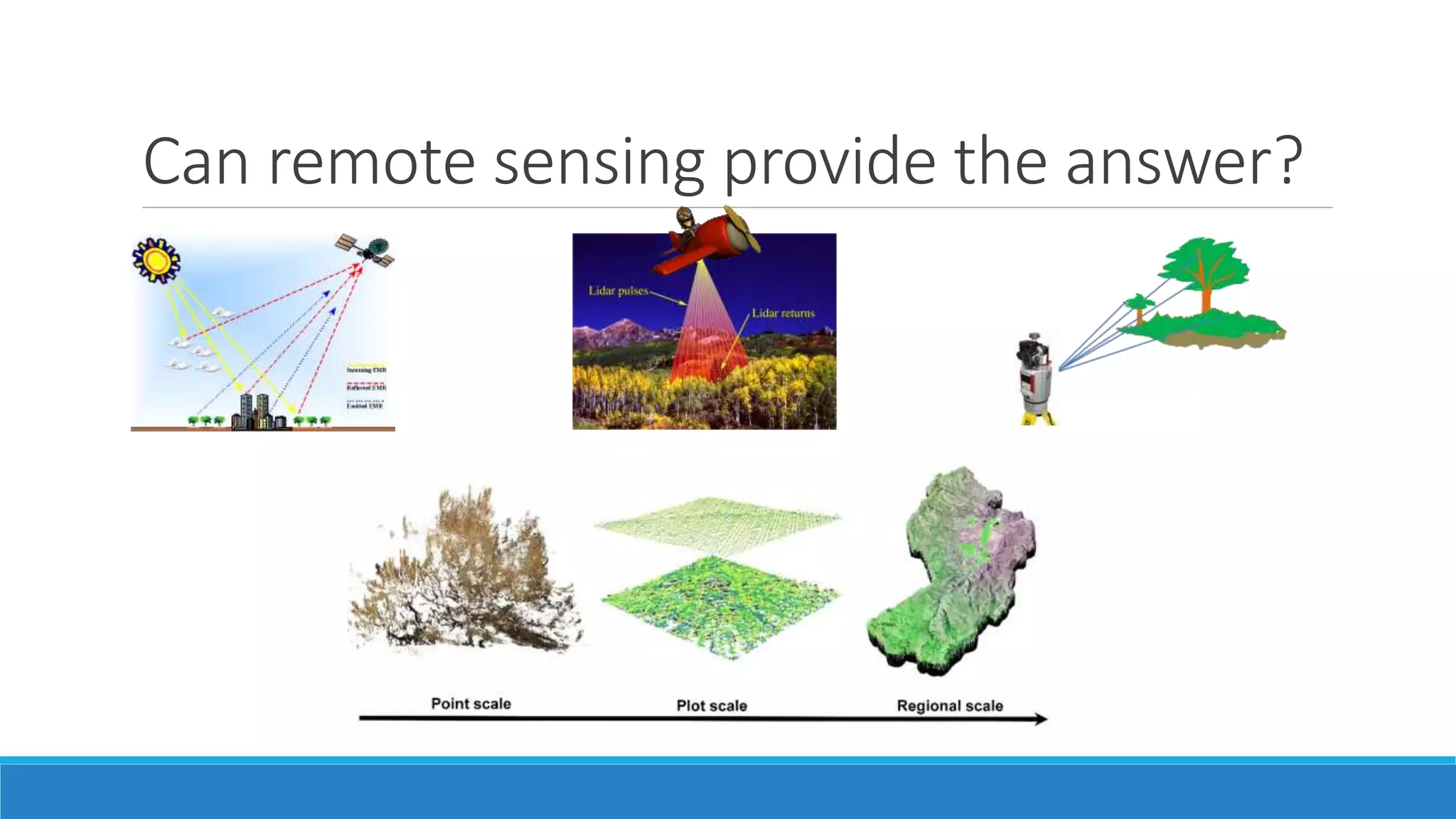
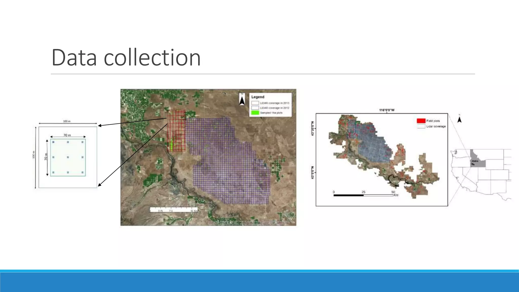
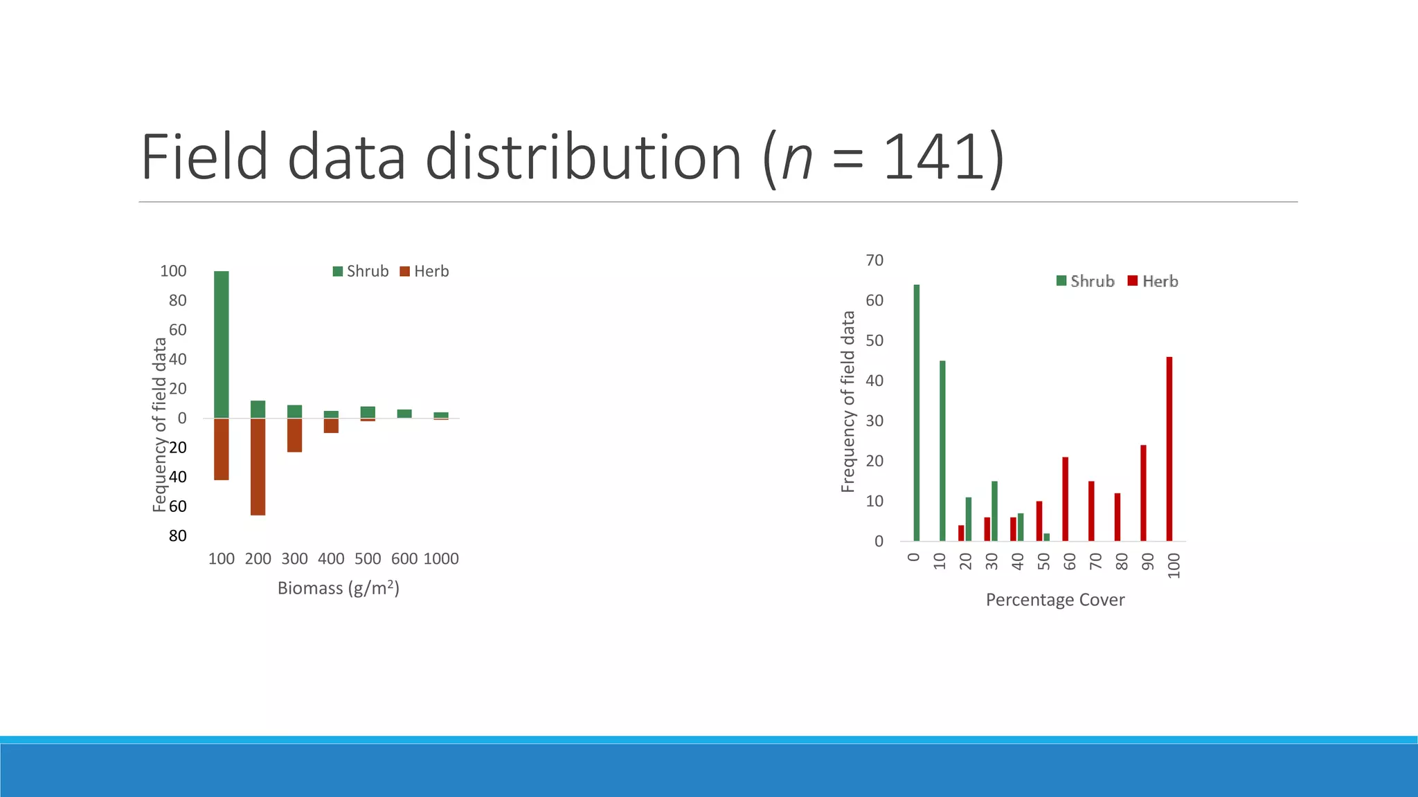
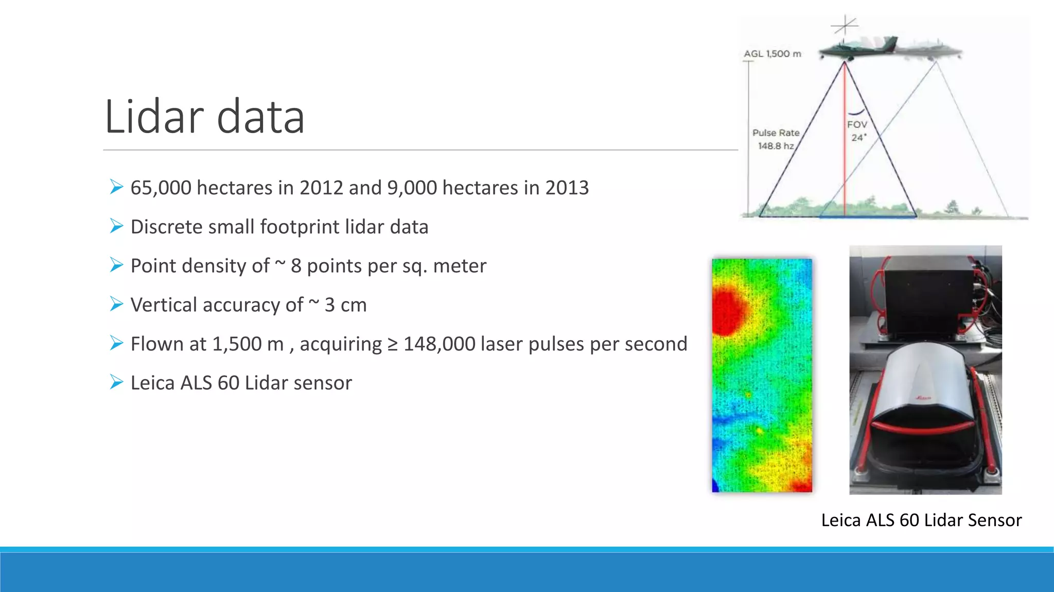
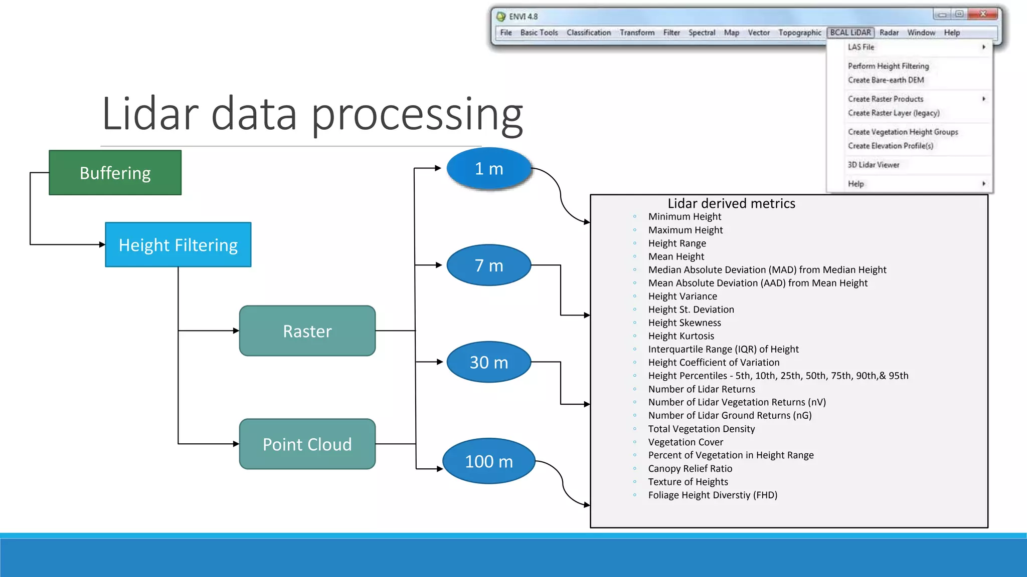
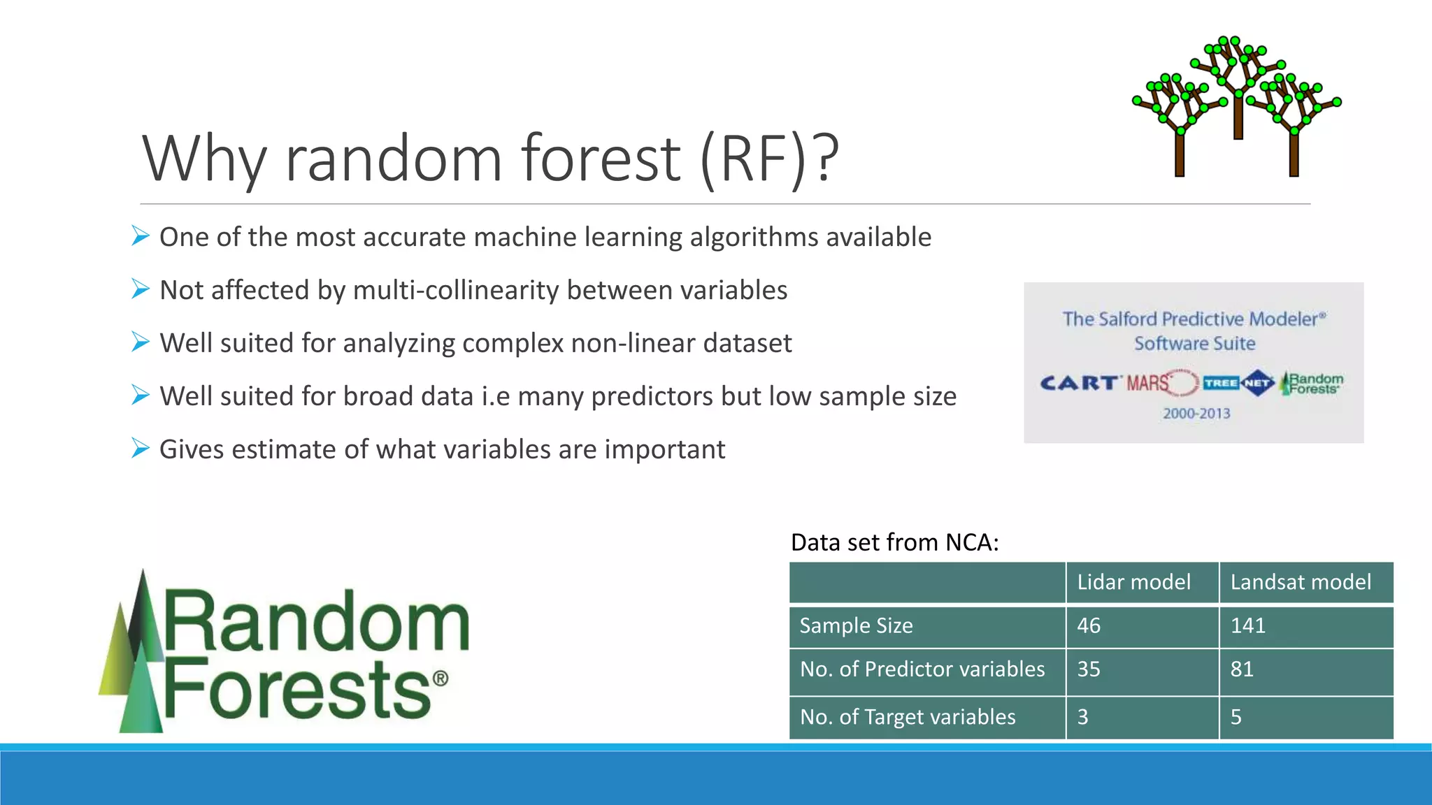
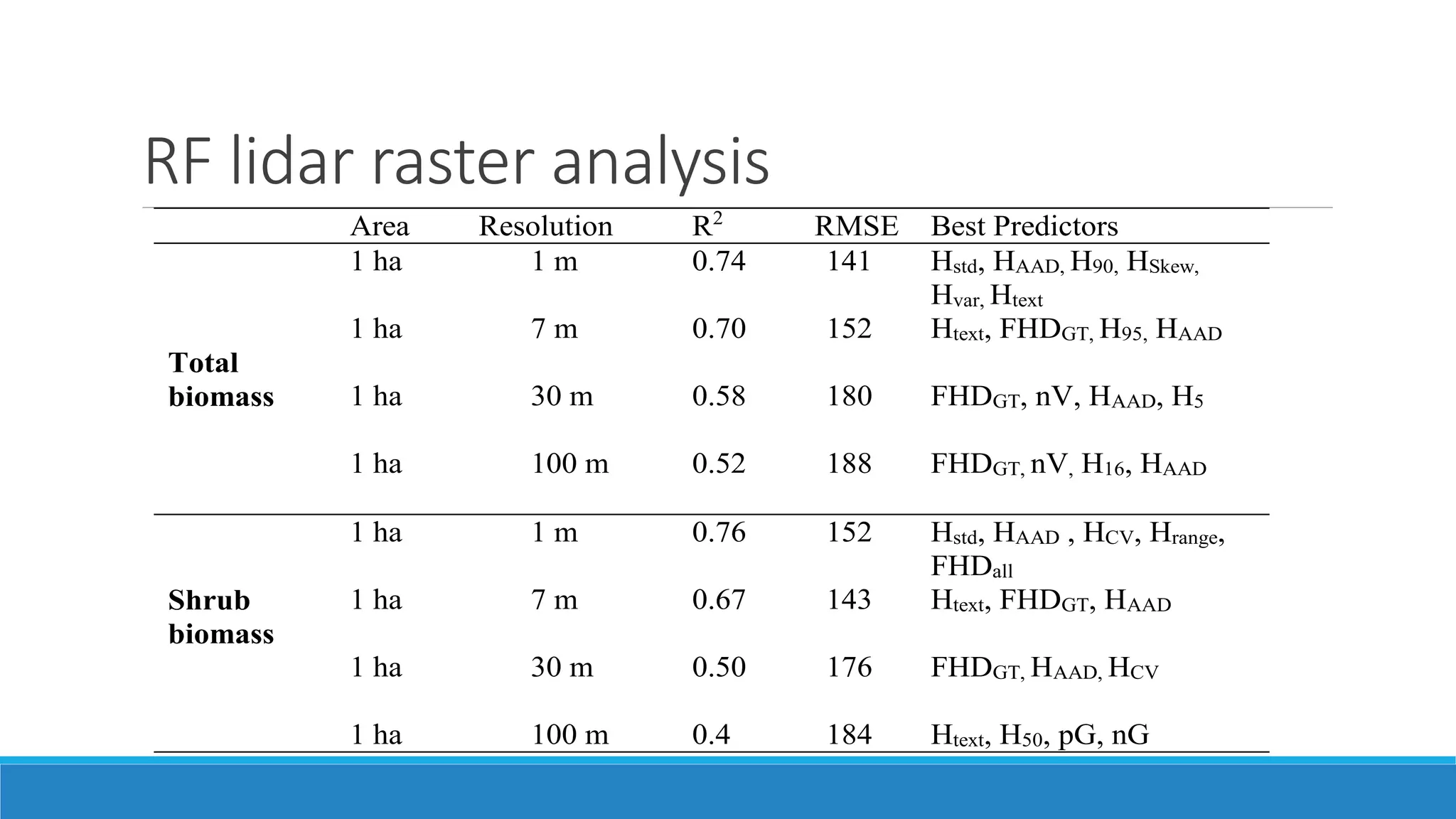
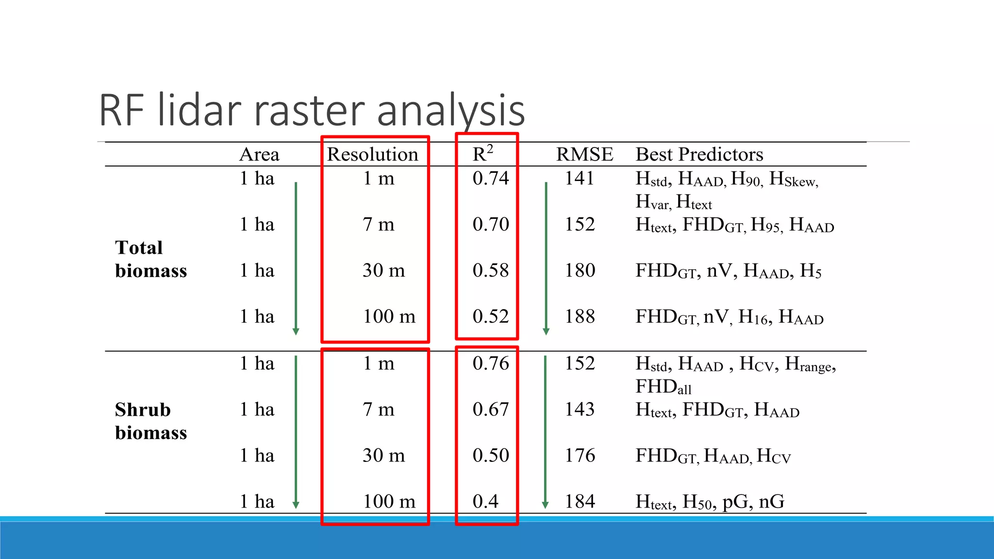
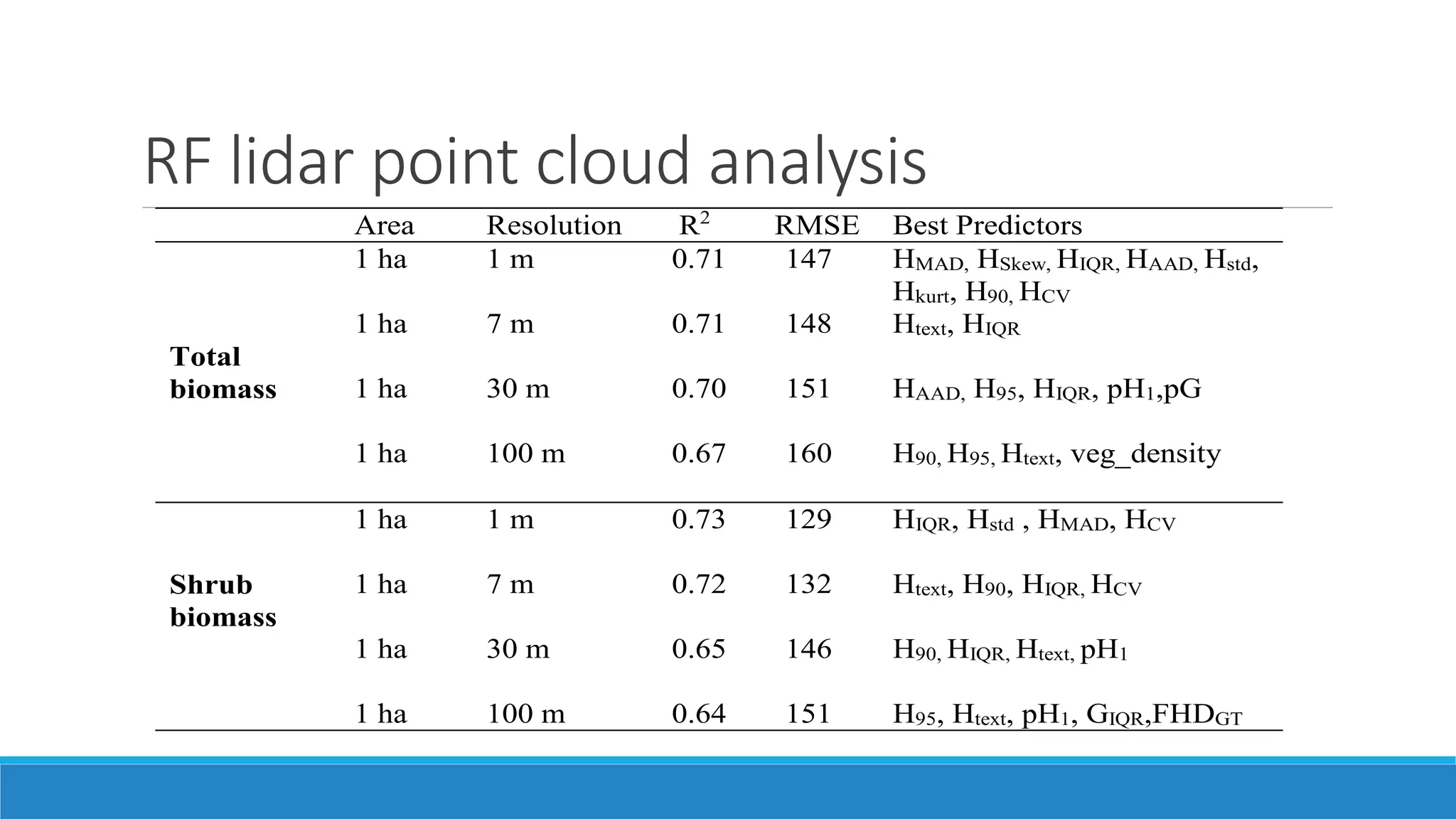
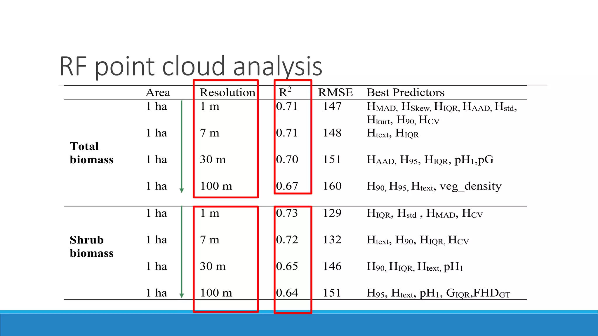
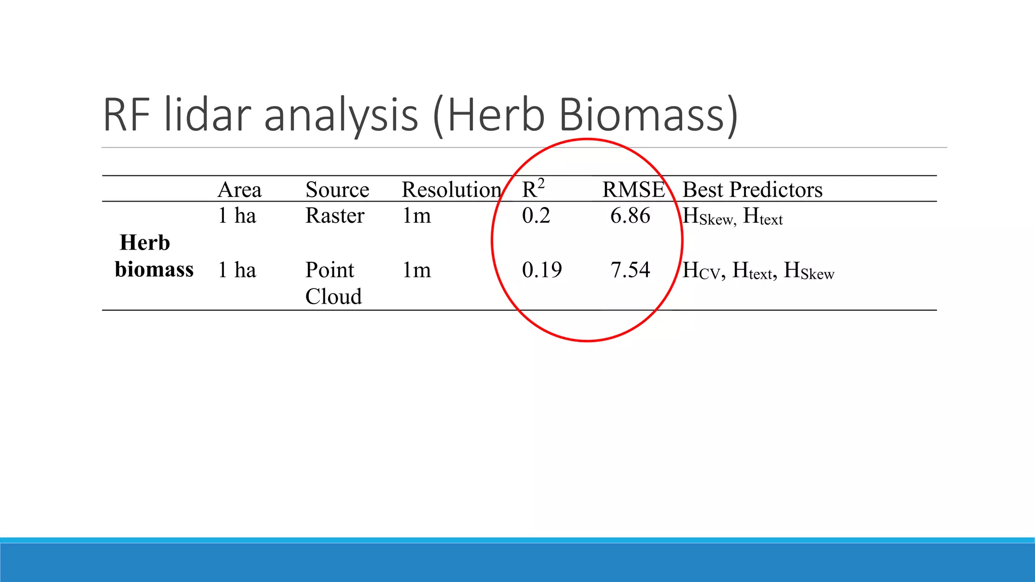
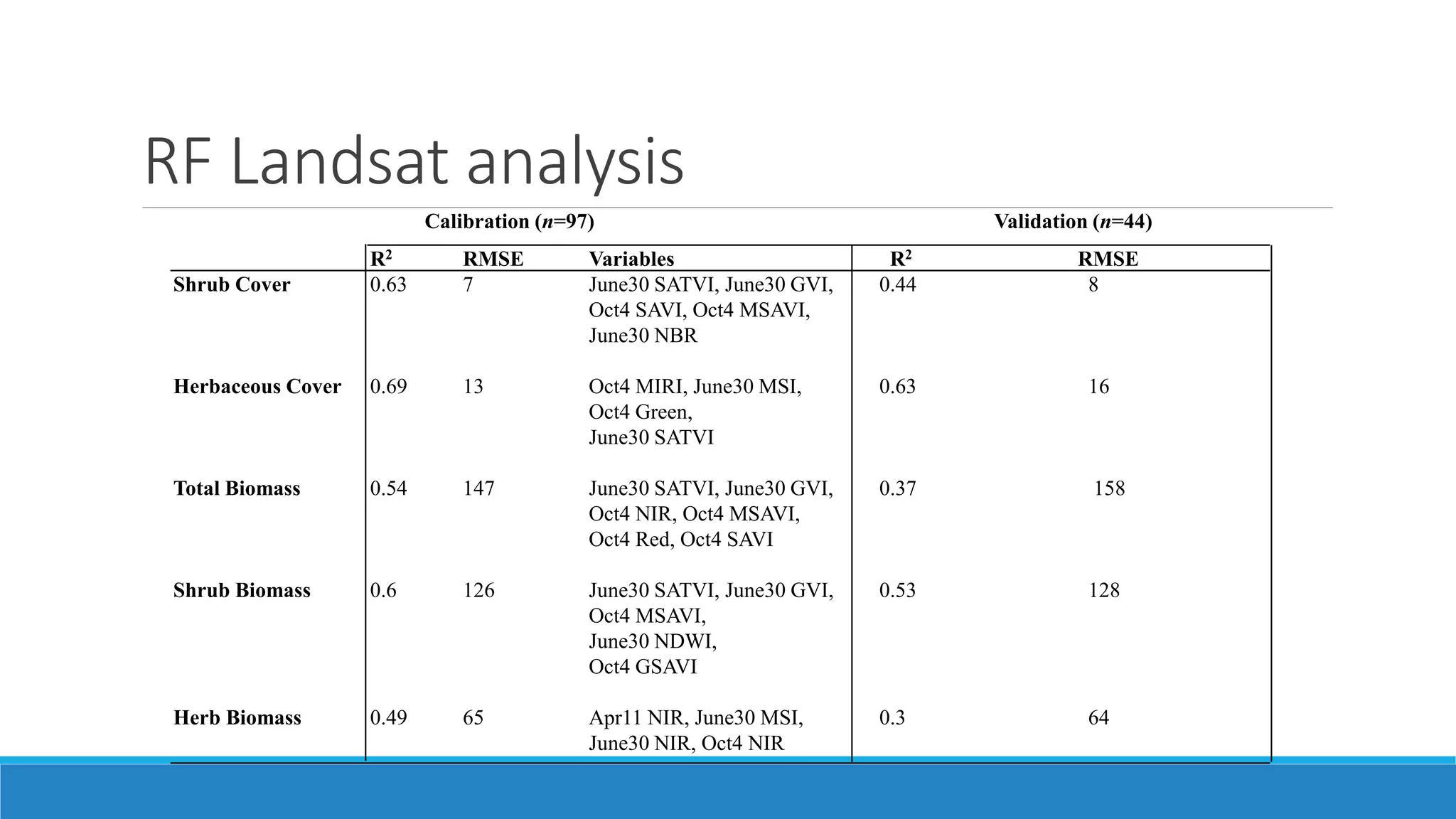
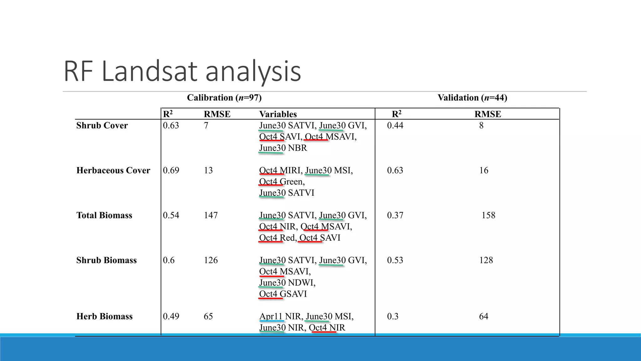
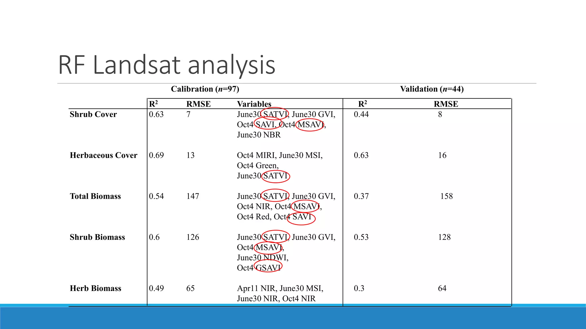
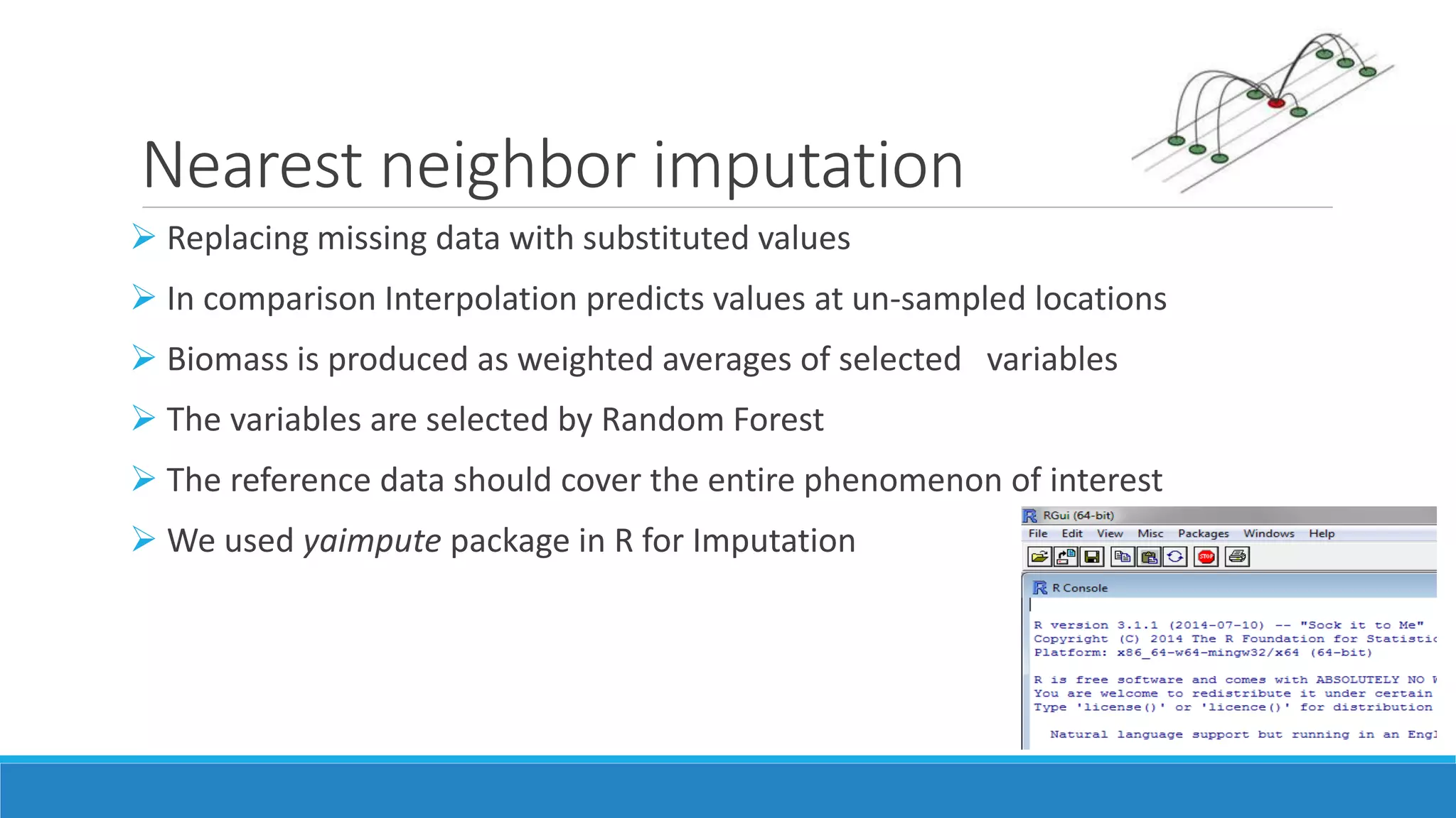
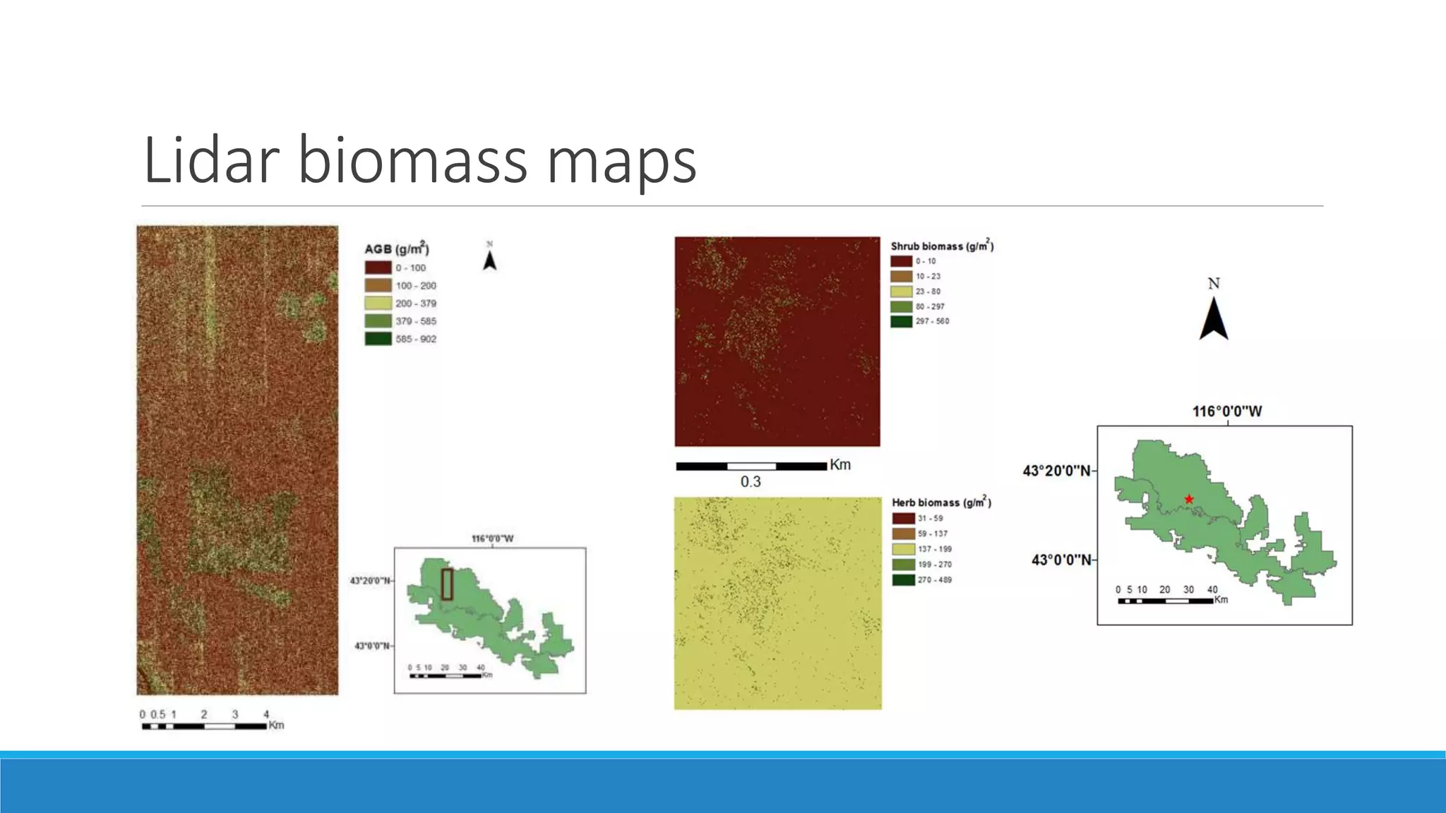
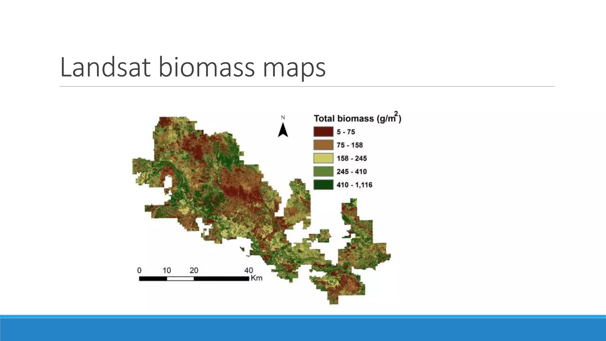
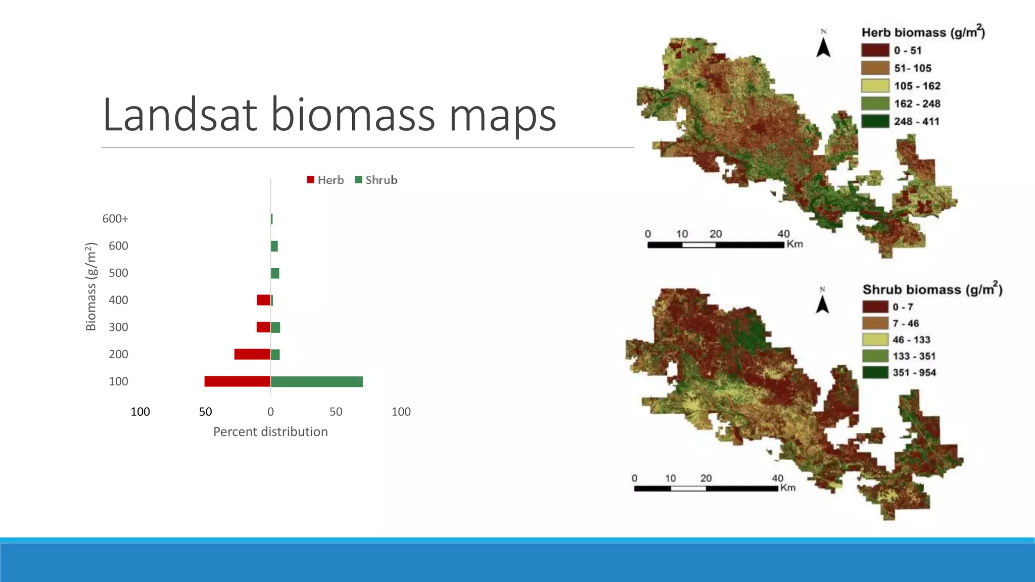
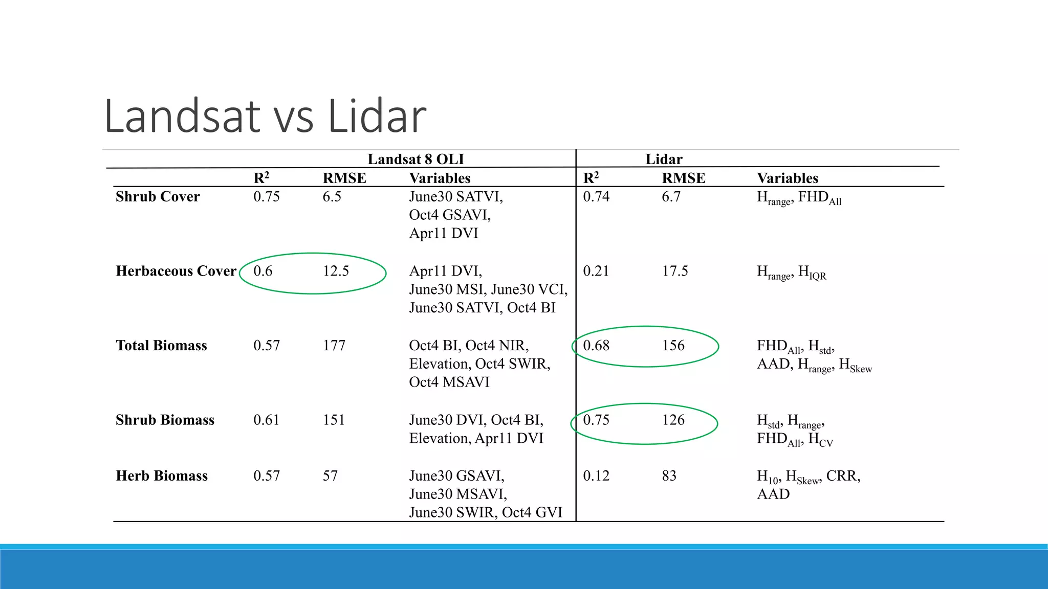
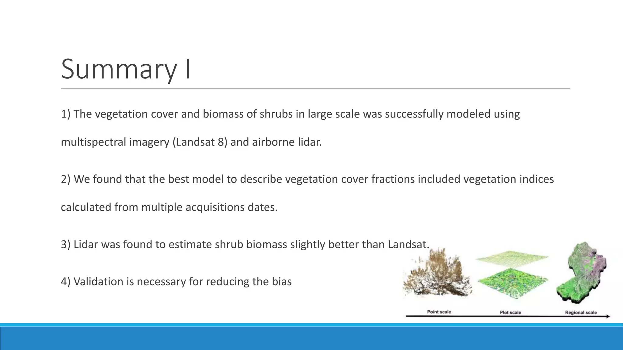
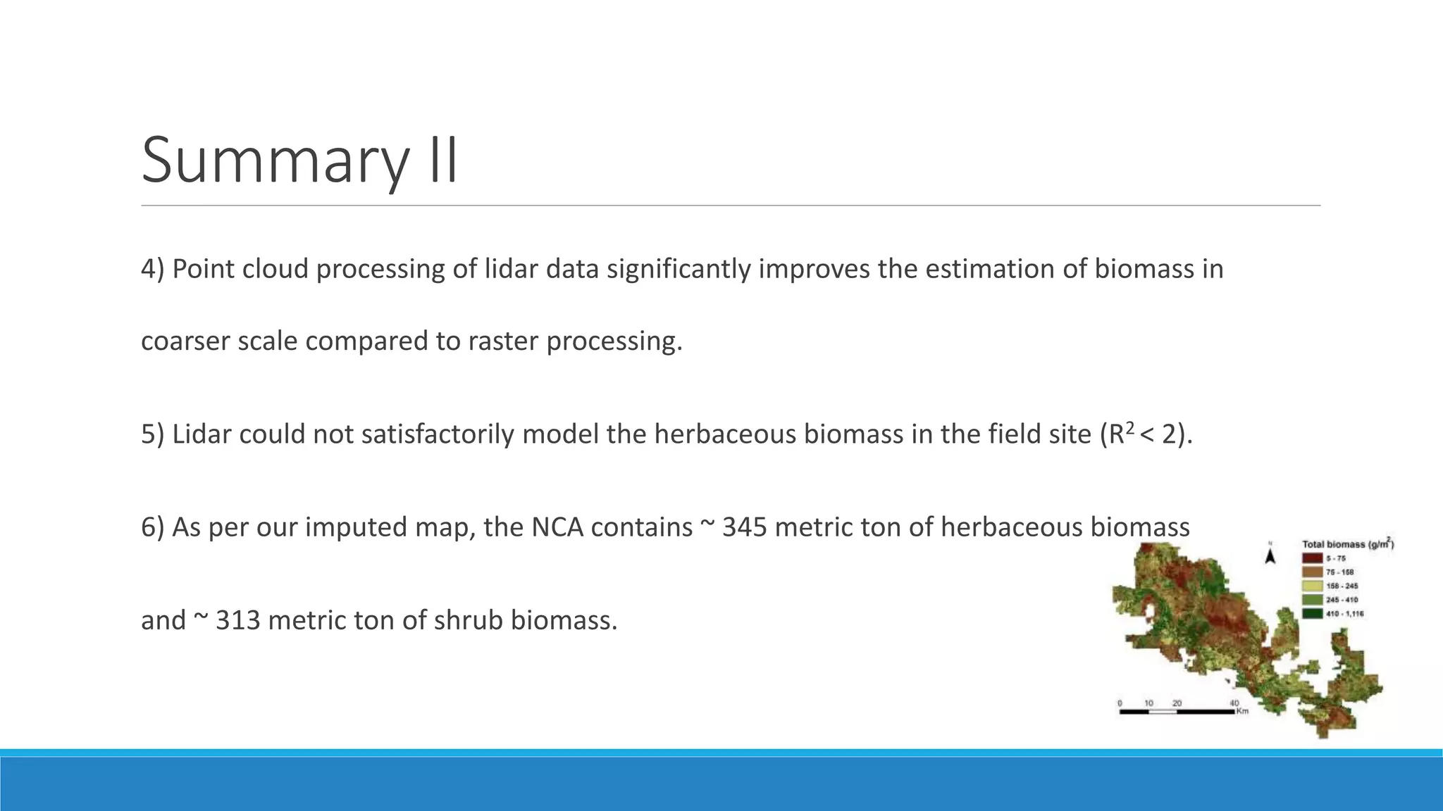
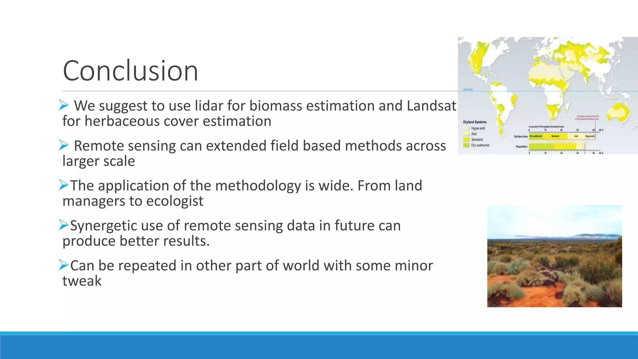
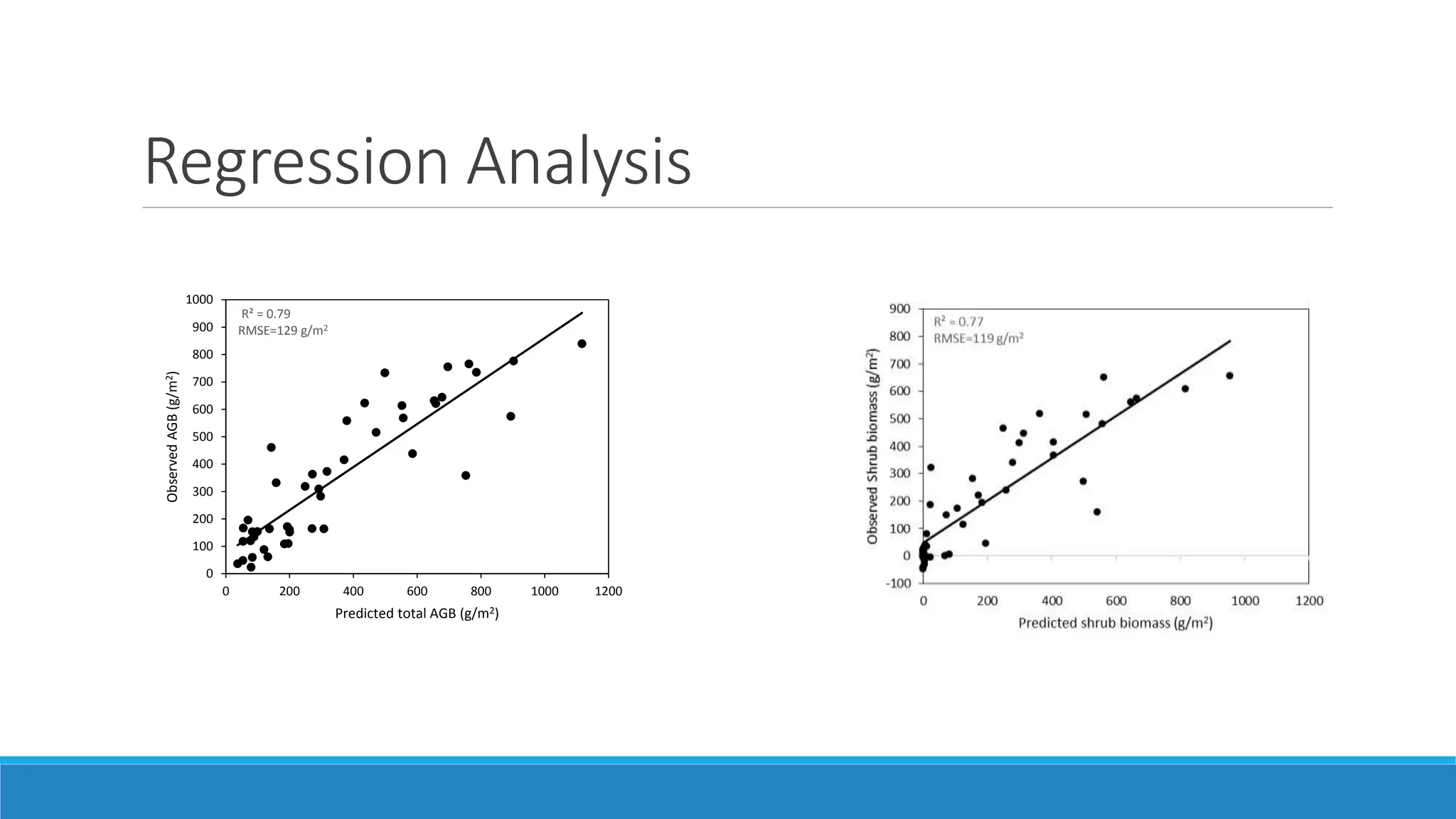
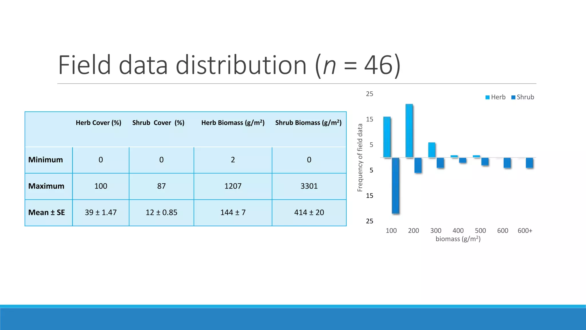
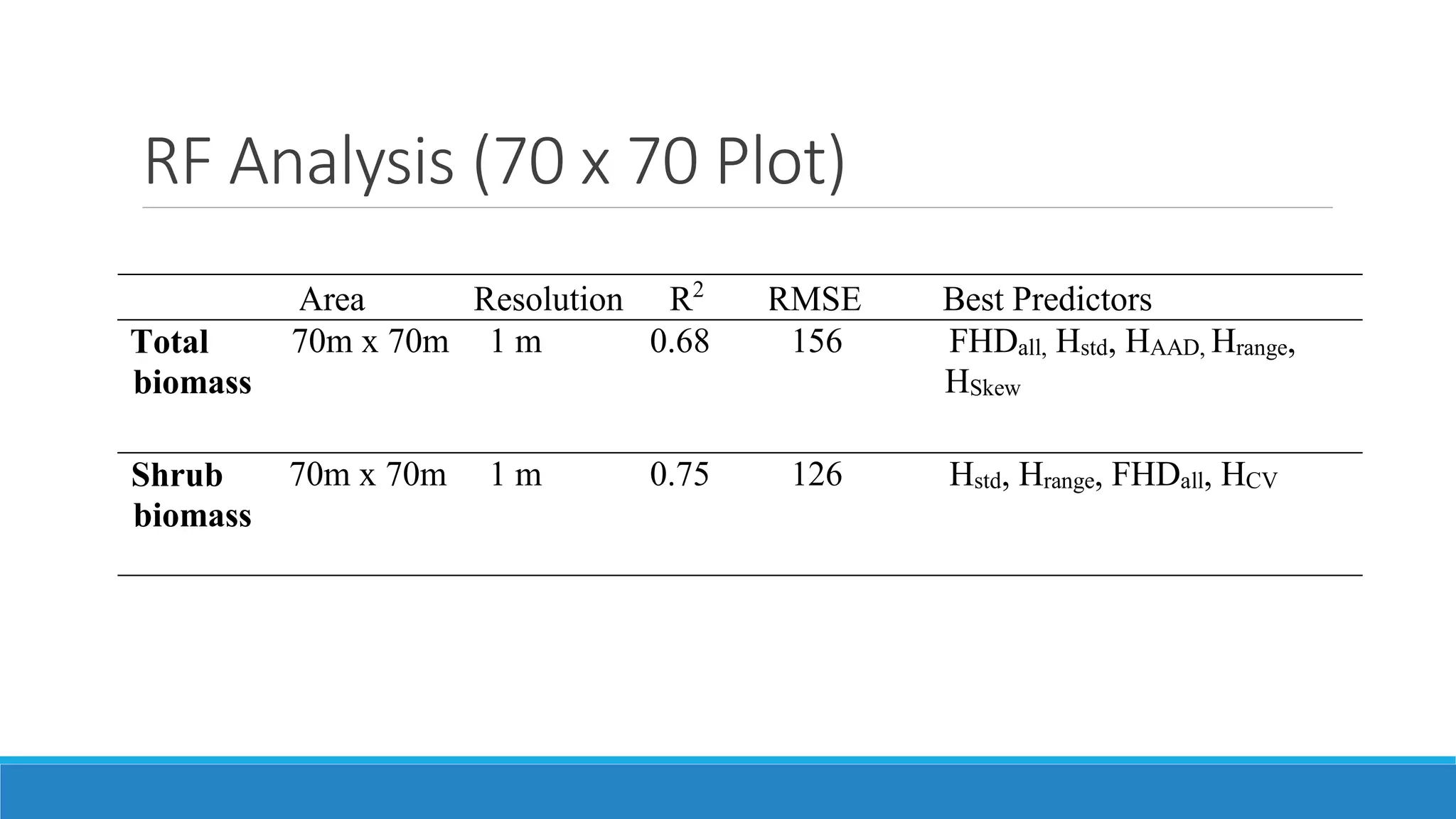
Assessing the Limitations and Capabilities of Lidar and Landsat
to Estimate Aboveground Vegetation Biomass and Cover in
Semi-arid Rangeland Ecosystem Using a Machine Learning
Algorithm
Shital Dhakal
MS in Hydrologic Sciences
Semi-arid ecosystem
Arid & Semi arid cover 1/3rd of Earth’s land surface
 These ecosystems are fragile due to water limitations
 Important roles in ecology, hydrology and carbon cycling
(PhotobyL.Engledow)
(PhotobyS.Hardegree)
Semi-arid in NW United States
Historically dominated by sagebrush steppe
One of the most important plants on western rangelands
Ecological, hydrological and carbon cycle importance
An imperiled ecosystem!
Reasons are increased fire frequency and replacement by exotic plants
Field based quantification
 Quantification is essential for modeling ecosystem, conservation of vegetation,
measuring fuel, understanding carbon flux etc.
 Some in-situ measurement methods are available
 E.g. Harvesting, Clip and Weigh, Visual estimation, Point intercept sampling
 Destructive method (clipping- oven drying) are expensive and labor intensive
 Point intercept sampling involves taking multiple field measurements
 Big problem- Very small geographical extent!
Can remote sensing provide the answer?
Previous studies
Hypothesis
 Satellite spectral remote sensing and Airborne Lidar can independently provide
large scale accurate estimation of vegetation characteristics in semi-arid rangeland.
Research questions
 What lidar based metrics are best to estimate biomass and cover of semi-arid vegetation ?
 Is point cloud processing of lidar data better than lidar based raster data?
 How does spectral remote sensing compare with lidar based estimation?
 What methods can be best utilized to produce biomass and cover map across a large scale?
 Can the available remote sensing technologies be used to estimate characteristics of both herbs and
shrubs in rangeland?
Outline of methodology
- Study site
- Field Data Collection
- Lidar data & Lidar data processing
-Landsat & Landsat image processing
-Random Forest
- Results from Lidar
-Results from Landsat
-Lidar vs Landsat
Study site
Morley Nelson Snake River Birds of Prey NCA, Boise
Data collection
Field data distribution (n = 141)
0
10
20
30
40
50
60
70
0
10
20
30
40
50
60
70
80
90
100
Frequencyoffielddata
Percentage Cover
80
60
40
20
0
20
40
60
80
100
100 200 300 400 500 600 1000
Fequencyoffielddata
Biomass (g/m2)
Shrub Herb
Lidar data
Leica ALS 60 Lidar Sensor
 65,000 hectares in 2012 and 9,000 hectares in 2013
 Discrete small footprint lidar data
 Point density of ~ 8 points per sq. meter
 Vertical accuracy of ~ 3 cm
 Flown at 1,500 m , acquiring ≥ 148,000 laser pulses per second
 Leica ALS 60 Lidar sensor
Lidar data processing
Lidar derived metrics
◦ Minimum Height
◦ Maximum Height
◦ Height Range
◦ Mean Height
◦ Median Absolute Deviation (MAD) from Median Height
◦ Mean Absolute Deviation (AAD) from Mean Height
◦ Height Variance
◦ Height St. Deviation
◦ Height Skewness
◦ Height Kurtosis
◦ Interquartile Range (IQR) of Height
◦ Height Coefficient of Variation
◦ Height Percentiles - 5th, 10th, 25th, 50th, 75th, 90th,& 95th
◦ Number of Lidar Returns
◦ Number of Lidar Vegetation Returns (nV)
◦ Number of Lidar Ground Returns (nG)
◦ Total Vegetation Density
◦ Vegetation Cover
◦ Percent of Vegetation in Height Range
◦ Canopy Relief Ratio
◦ Texture of Heights
◦ Foliage Height Diverstiy (FHD)
Buffering
Height Filtering
Raster
Point Cloud
1 m
7 m
30 m
100 m
Landsat 8 OLI
 Images the entire Earth every 16 days
 Spatial Resolution of 30 m
 Pushbroom Sensor
 Generates 16-bit images
 Eight fold increase in signal-to-noise ratio
Landsat 8 OLI
 Images the entire Earth every 16 days
 Spatial Resolution of 30 m
 Pushbroom Sensor
 Generates 16-bit images
 Eight fold increase in signal-to-noise ratio
Data Preparation (n=97+44)
11 Apr 2013
30 Jun 2013
4 Oct 2013
Topographic variables
Slope
Elevation
Aspect
More on vegetation indices
Simple Ratio based VI
-E.g. NDVI, SCI, VCI
Soil adjusted VI
-E.g. SAVI, GSAVI, SATVI
Perpendicular VI
-E.g. BI, GVI, WI
Why random forest (RF)?
 One of the most accurate machine learning algorithms available
 Not affected by multi-collinearity between variables
 Well suited for analyzing complex non-linear dataset
 Well suited for broad data i.e many predictors but low sample size
 Gives estimate of what variables are important
Lidar model Landsat model
Sample Size 46 141
No. of Predictor variables 35 81
No. of Target variables 3 5
Data set from NCA:
RF lidar raster analysis
Area Resolution R2
RMSE Best Predictors
Total
biomass
1 ha 1 m 0.74 141 Hstd, HAAD, H90, HSkew,
Hvar, Htext
1 ha 7 m 0.70 152 Htext, FHDGT, H95, HAAD
1 ha 30 m 0.58 180 FHDGT, nV, HAAD, H5
1 ha 100 m 0.52 188 FHDGT, nV, H16, HAAD
Shrub
biomass
1 ha 1 m 0.76 152 Hstd, HAAD , HCV, Hrange,
FHDall
1 ha 7 m 0.67 143 Htext, FHDGT, HAAD
1 ha 30 m 0.50 176 FHDGT, HAAD, HCV
1 ha 100 m 0.4 184 Htext, H50, pG, nG
RF lidar point cloud analysis
Area Resolution R2
RMSE Best Predictors
Total
biomass
1 ha 1 m 0.71 147 HMAD, HSkew, HIQR, HAAD, Hstd,
Hkurt, H90, HCV
1 ha 7 m 0.71 148 Htext, HIQR
1 ha 30 m 0.70 151 HAAD, H95, HIQR, pH1,pG
1 ha 100 m 0.67 160 H90, H95, Htext, veg_density
Shrub
biomass
1 ha 1 m 0.73 129 HIQR, Hstd , HMAD, HCV
1 ha 7 m 0.72 132 Htext, H90, HIQR, HCV
1 ha 30 m 0.65 146 H90, HIQR, Htext, pH1
1 ha 100 m 0.64 151 H95, Htext, pH1, GIQR,FHDGT
RF point cloud analysis
Area Resolution R2
RMSE Best Predictors
Total
biomass
1 ha 1 m 0.71 147 HMAD, HSkew, HIQR, HAAD, Hstd,
Hkurt, H90, HCV
1 ha 7 m 0.71 148 Htext, HIQR
1 ha 30 m 0.70 151 HAAD, H95, HIQR, pH1,pG
1 ha 100 m 0.67 160 H90, H95, Htext, veg_density
Shrub
biomass
1 ha 1 m 0.73 129 HIQR, Hstd , HMAD, HCV
1 ha 7 m 0.72 132 Htext, H90, HIQR, HCV
1 ha 30 m 0.65 146 H90, HIQR, Htext, pH1
1 ha 100 m 0.64 151 H95, Htext, pH1, GIQR,FHDGT
RF lidar analysis (Herb Biomass)
Area Source Resolution R2
RMSE Best Predictors
Herb
biomass
1 ha Raster 1m 0.2 6.86 HSkew, Htext
1 ha Point
Cloud
1m 0.19 7.54 HCV, Htext, HSkew
RF Landsat analysis
Calibration (n=97) Validation (n=44)
R2 RMSE Variables R2 RMSE
Shrub Cover 0.63 7 June30 SATVI, June30 GVI,
Oct4 SAVI, Oct4 MSAVI,
June30 NBR
0.44 8
Herbaceous Cover 0.69 13 Oct4 MIRI, June30 MSI,
Oct4 Green,
June30 SATVI
0.63 16
Total Biomass 0.54 147 June30 SATVI, June30 GVI,
Oct4 NIR, Oct4 MSAVI,
Oct4 Red, Oct4 SAVI
0.37 158
Shrub Biomass 0.6 126 June30 SATVI, June30 GVI,
Oct4 MSAVI,
June30 NDWI,
Oct4 GSAVI
0.53 128
Herb Biomass 0.49 65 Apr11 NIR, June30 MSI,
June30 NIR, Oct4 NIR
0.3 64
Nearest neighbor imputation
 Replacing missing data with substituted values
 In comparison Interpolation predicts values at un-sampled locations
 Biomass is produced as weighted averages of selected variables
 The variables are selected by Random Forest
 The reference data should cover the entire phenomenon of interest
 We used yaimpute package in R for Imputation
Lidar biomass maps
Landsat biomass maps
100 50 0 50 100
100
200
300
400
500
600
600+
Percent distribution
Biomass(g/m2)
Landsat cover maps
20 0 20 40 60 80
10
20
30
40
50
60
70
80
90
100
Percent distribution
PercentCover
Landsat vs Lidar
Landsat 8 OLI Lidar
R2 RMSE Variables R2 RMSE Variables
Shrub Cover 0.75 6.5 June30 SATVI,
Oct4 GSAVI,
Apr11 DVI
0.74 6.7 Hrange, FHDAll
Herbaceous Cover 0.6 12.5 Apr11 DVI,
June30 MSI, June30 VCI,
June30 SATVI, Oct4 BI
0.21 17.5 Hrange, HIQR
Total Biomass 0.57 177 Oct4 BI, Oct4 NIR,
Elevation, Oct4 SWIR,
Oct4 MSAVI
0.68 156 FHDAll, Hstd,
AAD, Hrange, HSkew
Shrub Biomass 0.61 151 June30 DVI, Oct4 BI,
Elevation, Apr11 DVI
0.75 126 Hstd, Hrange,
FHDAll, HCV
Herb Biomass 0.57 57 June30 GSAVI,
June30 MSAVI,
June30 SWIR, Oct4 GVI
0.12 83 H10, HSkew, CRR,
AAD
Summary I
1) The vegetation cover and biomass of shrubs in large scale was successfully modeled using
multispectral imagery (Landsat 8) and airborne lidar.
2) We found that the best model to describe vegetation cover fractions included vegetation indices
calculated from multiple acquisitions dates.
3) Lidar was found to estimate shrub biomass slightly better than Landsat.
4) Validation is necessary for reducing the bias
Summary II
4) Point cloud processing of lidar data significantly improves the estimation of biomass in
coarser scale compared to raster processing.
5) Lidar could not satisfactorily model the herbaceous biomass in the field site (R2 < 2).
6) As per our imputed map, the NCA contains ~ 345 metric ton of herbaceous biomass
and ~ 313 metric ton of shrub biomass.
An application - fire events
0
40
80
120
160
200
0 2 4 6 8 10
Averagebiomass(g/m2)
Fire frequency
Herb Shrub
0
20
40
60
80
0 2 4 6 8 10
Averagecover(%)
Fire frequency
Herb Shrub
0
50
100
150
200
250
300
0 2 4 6 8 10
Averagebiomass(g/m2)
Fire frequency
0
10
20
30
40
50
60
70
80
90
100
0 2 4 6 8 10
Averagecover(%)
Fire frequency
Herb
Shrub
With imputed pixels
With in-situ field plots
Conclusion
 We suggest to use lidar for biomass estimation and Landsat
for herbaceous cover estimation
 Remote sensing can extended field based methods across
larger scale
The application of the methodology is wide. From land
managers to ecologist
Synergetic use of remote sensing data in future can
produce better results.
Can be repeated in other part of world with some minor
tweak
Acknowledgement
 Committee chair- Dr. Nancy F. Glenn
Subject Committee – Dr. Alejandro N. Flores, Dr. Douglas J. Shinneman, Dr. Aihua Li
Dr. Rupesh Shrestha, Lucas Spaete
Peter Olsoy, Kyle Anderson, Hamid Dashti, Reggie, Ann Marie, Andrew, Katie
and Ginikanda Yapa Mudiyanselage Nayani Thanuja Ilangakoon
Nepalese friends and everyone in Geosciences!
Questions?
Regression Analysis
R² = 0.79
RMSE=129 g/m2
0
100
200
300
400
500
600
700
800
900
1000
0 200 400 600 800 1000 1200
ObservedAGB(g/m2)
Predicted total AGB (g/m2)
Field data distribution (n = 46)
Herb Cover (%) Shrub Cover (%) Herb Biomass (g/m2) Shrub Biomass (g/m2)
Minimum 0 0 2 0
Maximum 100 87 1207 3301
Mean ± SE 39 ± 1.47 12 ± 0.85 144 ± 7 414 ± 20
25
15
5
5
15
25
100 200 300 400 500 600 600+
Frequencyoffielddata
biomass (g/m2)
Herb Shrub
RF Analysis (70 x 70 Plot)
Area Resolution R2
RMSE Best Predictors
Total
biomass
70m x 70m 1 m 00.68 156 FHDall, Hstd, HAAD, Hrange,
HSkew
Shrub
biomass
70m x 70m 1 m 00.75 126 Hstd, Hrange, FHDall, HCV
extras

ASSESSING THE LIMITATIONS AND CAPABILITIES OF LIDAR AND LANDSAT 8 TO ESTIMATE THE ABOVEGROUND VEGETATION BIOMASS AND COVER IN A RANGELAND ECOSYSTEM USING A MACHINE LEARNING ALGORITHM

  • 1.
    Assessing the Limitationsand Capabilities of Lidar and Landsat to Estimate Aboveground Vegetation Biomass and Cover in Semi-arid Rangeland Ecosystem Using a Machine Learning Algorithm Shital Dhakal MS in Hydrologic Sciences
  • 2.
    Semi-arid ecosystem Arid &Semi arid cover 1/3rd of Earth’s land surface  These ecosystems are fragile due to water limitations  Important roles in ecology, hydrology and carbon cycling (PhotobyL.Engledow) (PhotobyS.Hardegree)
  • 3.
    Semi-arid in NWUnited States Historically dominated by sagebrush steppe One of the most important plants on western rangelands Ecological, hydrological and carbon cycle importance An imperiled ecosystem! Reasons are increased fire frequency and replacement by exotic plants
  • 4.
    Field based quantification Quantification is essential for modeling ecosystem, conservation of vegetation, measuring fuel, understanding carbon flux etc.  Some in-situ measurement methods are available  E.g. Harvesting, Clip and Weigh, Visual estimation, Point intercept sampling  Destructive method (clipping- oven drying) are expensive and labor intensive  Point intercept sampling involves taking multiple field measurements  Big problem- Very small geographical extent!
  • 5.
    Can remote sensingprovide the answer?
  • 6.
  • 7.
    Hypothesis  Satellite spectralremote sensing and Airborne Lidar can independently provide large scale accurate estimation of vegetation characteristics in semi-arid rangeland. Research questions  What lidar based metrics are best to estimate biomass and cover of semi-arid vegetation ?  Is point cloud processing of lidar data better than lidar based raster data?  How does spectral remote sensing compare with lidar based estimation?  What methods can be best utilized to produce biomass and cover map across a large scale?  Can the available remote sensing technologies be used to estimate characteristics of both herbs and shrubs in rangeland?
  • 8.
    Outline of methodology -Study site - Field Data Collection - Lidar data & Lidar data processing -Landsat & Landsat image processing -Random Forest - Results from Lidar -Results from Landsat -Lidar vs Landsat
  • 9.
    Study site Morley NelsonSnake River Birds of Prey NCA, Boise
  • 10.
  • 11.
    Field data distribution(n = 141) 0 10 20 30 40 50 60 70 0 10 20 30 40 50 60 70 80 90 100 Frequencyoffielddata Percentage Cover 80 60 40 20 0 20 40 60 80 100 100 200 300 400 500 600 1000 Fequencyoffielddata Biomass (g/m2) Shrub Herb
  • 12.
    Lidar data Leica ALS60 Lidar Sensor  65,000 hectares in 2012 and 9,000 hectares in 2013  Discrete small footprint lidar data  Point density of ~ 8 points per sq. meter  Vertical accuracy of ~ 3 cm  Flown at 1,500 m , acquiring ≥ 148,000 laser pulses per second  Leica ALS 60 Lidar sensor
  • 13.
    Lidar data processing Lidarderived metrics ◦ Minimum Height ◦ Maximum Height ◦ Height Range ◦ Mean Height ◦ Median Absolute Deviation (MAD) from Median Height ◦ Mean Absolute Deviation (AAD) from Mean Height ◦ Height Variance ◦ Height St. Deviation ◦ Height Skewness ◦ Height Kurtosis ◦ Interquartile Range (IQR) of Height ◦ Height Coefficient of Variation ◦ Height Percentiles - 5th, 10th, 25th, 50th, 75th, 90th,& 95th ◦ Number of Lidar Returns ◦ Number of Lidar Vegetation Returns (nV) ◦ Number of Lidar Ground Returns (nG) ◦ Total Vegetation Density ◦ Vegetation Cover ◦ Percent of Vegetation in Height Range ◦ Canopy Relief Ratio ◦ Texture of Heights ◦ Foliage Height Diverstiy (FHD) Buffering Height Filtering Raster Point Cloud 1 m 7 m 30 m 100 m
  • 14.
    Landsat 8 OLI Images the entire Earth every 16 days  Spatial Resolution of 30 m  Pushbroom Sensor  Generates 16-bit images  Eight fold increase in signal-to-noise ratio
  • 15.
    Landsat 8 OLI Images the entire Earth every 16 days  Spatial Resolution of 30 m  Pushbroom Sensor  Generates 16-bit images  Eight fold increase in signal-to-noise ratio
  • 16.
    Data Preparation (n=97+44) 11Apr 2013 30 Jun 2013 4 Oct 2013 Topographic variables Slope Elevation Aspect
  • 17.
    More on vegetationindices Simple Ratio based VI -E.g. NDVI, SCI, VCI Soil adjusted VI -E.g. SAVI, GSAVI, SATVI Perpendicular VI -E.g. BI, GVI, WI
  • 18.
    Why random forest(RF)?  One of the most accurate machine learning algorithms available  Not affected by multi-collinearity between variables  Well suited for analyzing complex non-linear dataset  Well suited for broad data i.e many predictors but low sample size  Gives estimate of what variables are important Lidar model Landsat model Sample Size 46 141 No. of Predictor variables 35 81 No. of Target variables 3 5 Data set from NCA:
  • 19.
    RF lidar rasteranalysis Area Resolution R2 RMSE Best Predictors Total biomass 1 ha 1 m 0.74 141 Hstd, HAAD, H90, HSkew, Hvar, Htext 1 ha 7 m 0.70 152 Htext, FHDGT, H95, HAAD 1 ha 30 m 0.58 180 FHDGT, nV, HAAD, H5 1 ha 100 m 0.52 188 FHDGT, nV, H16, HAAD Shrub biomass 1 ha 1 m 0.76 152 Hstd, HAAD , HCV, Hrange, FHDall 1 ha 7 m 0.67 143 Htext, FHDGT, HAAD 1 ha 30 m 0.50 176 FHDGT, HAAD, HCV 1 ha 100 m 0.4 184 Htext, H50, pG, nG
  • 20.
    RF lidar rasteranalysis Area Resolution R2 RMSE Best Predictors Total biomass 1 ha 1 m 0.74 141 Hstd, HAAD, H90, HSkew, Hvar, Htext 1 ha 7 m 0.70 152 Htext, FHDGT, H95, HAAD 1 ha 30 m 0.58 180 FHDGT, nV, HAAD, H5 1 ha 100 m 0.52 188 FHDGT, nV, H16, HAAD Shrub biomass 1 ha 1 m 0.76 152 Hstd, HAAD , HCV, Hrange, FHDall 1 ha 7 m 0.67 143 Htext, FHDGT, HAAD 1 ha 30 m 0.50 176 FHDGT, HAAD, HCV 1 ha 100 m 0.4 184 Htext, H50, pG, nG
  • 21.
    RF lidar pointcloud analysis Area Resolution R2 RMSE Best Predictors Total biomass 1 ha 1 m 0.71 147 HMAD, HSkew, HIQR, HAAD, Hstd, Hkurt, H90, HCV 1 ha 7 m 0.71 148 Htext, HIQR 1 ha 30 m 0.70 151 HAAD, H95, HIQR, pH1,pG 1 ha 100 m 0.67 160 H90, H95, Htext, veg_density Shrub biomass 1 ha 1 m 0.73 129 HIQR, Hstd , HMAD, HCV 1 ha 7 m 0.72 132 Htext, H90, HIQR, HCV 1 ha 30 m 0.65 146 H90, HIQR, Htext, pH1 1 ha 100 m 0.64 151 H95, Htext, pH1, GIQR,FHDGT
  • 22.
    RF point cloudanalysis Area Resolution R2 RMSE Best Predictors Total biomass 1 ha 1 m 0.71 147 HMAD, HSkew, HIQR, HAAD, Hstd, Hkurt, H90, HCV 1 ha 7 m 0.71 148 Htext, HIQR 1 ha 30 m 0.70 151 HAAD, H95, HIQR, pH1,pG 1 ha 100 m 0.67 160 H90, H95, Htext, veg_density Shrub biomass 1 ha 1 m 0.73 129 HIQR, Hstd , HMAD, HCV 1 ha 7 m 0.72 132 Htext, H90, HIQR, HCV 1 ha 30 m 0.65 146 H90, HIQR, Htext, pH1 1 ha 100 m 0.64 151 H95, Htext, pH1, GIQR,FHDGT
  • 23.
    RF lidar analysis(Herb Biomass) Area Source Resolution R2 RMSE Best Predictors Herb biomass 1 ha Raster 1m 0.2 6.86 HSkew, Htext 1 ha Point Cloud 1m 0.19 7.54 HCV, Htext, HSkew
  • 24.
    RF Landsat analysis Calibration(n=97) Validation (n=44) R2 RMSE Variables R2 RMSE Shrub Cover 0.63 7 June30 SATVI, June30 GVI, Oct4 SAVI, Oct4 MSAVI, June30 NBR 0.44 8 Herbaceous Cover 0.69 13 Oct4 MIRI, June30 MSI, Oct4 Green, June30 SATVI 0.63 16 Total Biomass 0.54 147 June30 SATVI, June30 GVI, Oct4 NIR, Oct4 MSAVI, Oct4 Red, Oct4 SAVI 0.37 158 Shrub Biomass 0.6 126 June30 SATVI, June30 GVI, Oct4 MSAVI, June30 NDWI, Oct4 GSAVI 0.53 128 Herb Biomass 0.49 65 Apr11 NIR, June30 MSI, June30 NIR, Oct4 NIR 0.3 64
  • 25.
    RF Landsat analysis Calibration(n=97) Validation (n=44) R2 RMSE Variables R2 RMSE Shrub Cover 0.63 7 June30 SATVI, June30 GVI, Oct4 SAVI, Oct4 MSAVI, June30 NBR 0.44 8 Herbaceous Cover 0.69 13 Oct4 MIRI, June30 MSI, Oct4 Green, June30 SATVI 0.63 16 Total Biomass 0.54 147 June30 SATVI, June30 GVI, Oct4 NIR, Oct4 MSAVI, Oct4 Red, Oct4 SAVI 0.37 158 Shrub Biomass 0.6 126 June30 SATVI, June30 GVI, Oct4 MSAVI, June30 NDWI, Oct4 GSAVI 0.53 128 Herb Biomass 0.49 65 Apr11 NIR, June30 MSI, June30 NIR, Oct4 NIR 0.3 64
  • 26.
    RF Landsat analysis Calibration(n=97) Validation (n=44) R2 RMSE Variables R2 RMSE Shrub Cover 0.63 7 June30 SATVI, June30 GVI, Oct4 SAVI, Oct4 MSAVI, June30 NBR 0.44 8 Herbaceous Cover 0.69 13 Oct4 MIRI, June30 MSI, Oct4 Green, June30 SATVI 0.63 16 Total Biomass 0.54 147 June30 SATVI, June30 GVI, Oct4 NIR, Oct4 MSAVI, Oct4 Red, Oct4 SAVI 0.37 158 Shrub Biomass 0.6 126 June30 SATVI, June30 GVI, Oct4 MSAVI, June30 NDWI, Oct4 GSAVI 0.53 128 Herb Biomass 0.49 65 Apr11 NIR, June30 MSI, June30 NIR, Oct4 NIR 0.3 64
  • 27.
    Nearest neighbor imputation Replacing missing data with substituted values  In comparison Interpolation predicts values at un-sampled locations  Biomass is produced as weighted averages of selected variables  The variables are selected by Random Forest  The reference data should cover the entire phenomenon of interest  We used yaimpute package in R for Imputation
  • 28.
  • 29.
  • 30.
    Landsat biomass maps 10050 0 50 100 100 200 300 400 500 600 600+ Percent distribution Biomass(g/m2)
  • 31.
    Landsat cover maps 200 20 40 60 80 10 20 30 40 50 60 70 80 90 100 Percent distribution PercentCover
  • 32.
    Landsat vs Lidar Landsat8 OLI Lidar R2 RMSE Variables R2 RMSE Variables Shrub Cover 0.75 6.5 June30 SATVI, Oct4 GSAVI, Apr11 DVI 0.74 6.7 Hrange, FHDAll Herbaceous Cover 0.6 12.5 Apr11 DVI, June30 MSI, June30 VCI, June30 SATVI, Oct4 BI 0.21 17.5 Hrange, HIQR Total Biomass 0.57 177 Oct4 BI, Oct4 NIR, Elevation, Oct4 SWIR, Oct4 MSAVI 0.68 156 FHDAll, Hstd, AAD, Hrange, HSkew Shrub Biomass 0.61 151 June30 DVI, Oct4 BI, Elevation, Apr11 DVI 0.75 126 Hstd, Hrange, FHDAll, HCV Herb Biomass 0.57 57 June30 GSAVI, June30 MSAVI, June30 SWIR, Oct4 GVI 0.12 83 H10, HSkew, CRR, AAD
  • 33.
    Summary I 1) Thevegetation cover and biomass of shrubs in large scale was successfully modeled using multispectral imagery (Landsat 8) and airborne lidar. 2) We found that the best model to describe vegetation cover fractions included vegetation indices calculated from multiple acquisitions dates. 3) Lidar was found to estimate shrub biomass slightly better than Landsat. 4) Validation is necessary for reducing the bias
  • 34.
    Summary II 4) Pointcloud processing of lidar data significantly improves the estimation of biomass in coarser scale compared to raster processing. 5) Lidar could not satisfactorily model the herbaceous biomass in the field site (R2 < 2). 6) As per our imputed map, the NCA contains ~ 345 metric ton of herbaceous biomass and ~ 313 metric ton of shrub biomass.
  • 35.
    An application -fire events 0 40 80 120 160 200 0 2 4 6 8 10 Averagebiomass(g/m2) Fire frequency Herb Shrub 0 20 40 60 80 0 2 4 6 8 10 Averagecover(%) Fire frequency Herb Shrub 0 50 100 150 200 250 300 0 2 4 6 8 10 Averagebiomass(g/m2) Fire frequency 0 10 20 30 40 50 60 70 80 90 100 0 2 4 6 8 10 Averagecover(%) Fire frequency Herb Shrub With imputed pixels With in-situ field plots
  • 36.
    Conclusion  We suggestto use lidar for biomass estimation and Landsat for herbaceous cover estimation  Remote sensing can extended field based methods across larger scale The application of the methodology is wide. From land managers to ecologist Synergetic use of remote sensing data in future can produce better results. Can be repeated in other part of world with some minor tweak
  • 37.
    Acknowledgement  Committee chair-Dr. Nancy F. Glenn Subject Committee – Dr. Alejandro N. Flores, Dr. Douglas J. Shinneman, Dr. Aihua Li Dr. Rupesh Shrestha, Lucas Spaete Peter Olsoy, Kyle Anderson, Hamid Dashti, Reggie, Ann Marie, Andrew, Katie and Ginikanda Yapa Mudiyanselage Nayani Thanuja Ilangakoon Nepalese friends and everyone in Geosciences!
  • 38.
  • 40.
    Regression Analysis R² =0.79 RMSE=129 g/m2 0 100 200 300 400 500 600 700 800 900 1000 0 200 400 600 800 1000 1200 ObservedAGB(g/m2) Predicted total AGB (g/m2)
  • 41.
    Field data distribution(n = 46) Herb Cover (%) Shrub Cover (%) Herb Biomass (g/m2) Shrub Biomass (g/m2) Minimum 0 0 2 0 Maximum 100 87 1207 3301 Mean ± SE 39 ± 1.47 12 ± 0.85 144 ± 7 414 ± 20 25 15 5 5 15 25 100 200 300 400 500 600 600+ Frequencyoffielddata biomass (g/m2) Herb Shrub
  • 42.
    RF Analysis (70x 70 Plot) Area Resolution R2 RMSE Best Predictors Total biomass 70m x 70m 1 m 00.68 156 FHDall, Hstd, HAAD, Hrange, HSkew Shrub biomass 70m x 70m 1 m 00.75 126 Hstd, Hrange, FHDall, HCV
  • 43.

Editor's Notes

  • #2 Introduce Committee
  • #3 Typical Karoo vegetation to the south of Matjiesfontein, with the Anysberg Mountains visible in the background WPPs are found in the Middleback Ranges; a semi-arid mallee system, with a eucalypt upperstorey and hummock grass (Triodia irritans) dominated understory. (Photo by L. Engledow)
  • #4 Native shrubs like sagebrush are one of the most important plants on western rangelands from an ecological point of view. They are home and provide food to endangered animals like greater sage grouse (Centrocercus urophasianus) and pygmy rabbits (Brachylagus idahoensis) (Storch 2007; Shipley et al. 2006; J. W. Connelly et al. 2000). Sagebrush provides habitat for nearly 100 types of birds and to hosts of invertebrates which in turn support birds, reptiles and small mammals. Thermal or security cover is also provided by sagebrush for wildlife like pheasants, chukar, sharp tailed grouse and sage grouse. A change in the sagebrush distribution will cause a decline in number of these already endangered species and species that are not yet endangered. Distribution of sagebrush across the rangeland is also important from hydrology and hydraulics point of view (Ursino 2007; Pierson et al. 2003). Big sagebrush plants have a two-part root system- deep tap root and a shallow diffuse root system. The tap root system brings deep soil moisture and nutrients to the soil surface by “hydraulic lift” which is available for roots of other understory plants (Cardon et al. 2013). This decreases water holding capacity of soil and infiltration and increases the surface flow. Sagebrush plays a crucial role in the hydrological cycle of the water-limited region (Wilcox 2010). Evapotranspiration is a major component of soil water content in semiarid rangeland and about 96% of incoming precipitation has been shown to be returned to the atmosphere by vegetation such as sagebrush in rangelands (Branson, Miller, and McQueen 1976). Several studies (Angell et al. 2001; Shrestha and Stahl 2008) have also shown the critical role that sagebrush plays as a storage of terrestrial carbon storage.
  • #6 The LiDAR instrument fires rapid pulses of laser light at a surface, some at up to 150,000 pulses per second. A sensor on the instrument measures the amount of time it takes for each pulse to bounce back. Light moves at a constant and known speed so the LiDAR instrument can calculate the distance between itself and the target with high accuracy. By repeating this in quick succession the instrument builds up a complex 'map' of the surface it is measuring.
  • #7 Zolkos- 70 referred articles for optical, lidar and radar Hufkens- Upscaling of RS data using averaged LAI in China Chen et al.- Used 17 vegetative indices in estimating saltbush and total vegetation cover in Australia using Landsat TM Vierling et al- Used TLS to automatically determine structural information of individual shrub in WA Zandler et al- Modeled total biomass in Tajikistan using Landsat and Rapid eye using several modeling approaches- stepwise, lasso, pls, RF etc.
  • #10 The study area is located within the Morley Nelson Snake River Birds of Prey National Conservation Area (NCA), a shrub-steppe rangeland once dominated by big sagebrush. The NCA encompasses about 600,000 acres of the Snake River Plain ecoregion in southwestern Idaho, USA . It contains other native species including shadescale (Altriplex confertifolia), winterfat (Ceratoides lanata), budsage (Artemisia spinescen), and rabbitbrush (Chrysothamnus visciflorus) including rapidly invading annual exotic like cheatgrass (Bromus tectorum). Since 1980, over half of the NCA has been burned resulting a mosaic of plant communities, with compositions spanning a gradient between intact native shrublands, shrublands degraded by biological invasion and wildfire, and grasslands where native plants have been fully replaced by cheatgrass and other invasive annuals. Currently 37% or less of the NCA retains an intact a native shrubland community
  • #11 Talk about 1)Clipping and oven drying 1.5)Grouping into categories 2)Averaging the biomass and cover in subplots 3)Define herbs
  • #12 Talk about calibration and validation plots (97+44)
  • #15  A push broom scanner can gather morelight than a whisk broom scanner because it looks at a particular area for a longer time, like a long exposure on a camera.
  • #17 -We first acquired images overlapping the study site -derived vegetation indices for each of the plot Talk about why did you choose these dates? – overlapping with field dates, low cloud cover and acquisition of Landsat 8 Why these particular vegetation indices? Why topographic variables? And why RF again? SRTM DEM- Shuttle Radar Topography DEMv(90 m)
  • #19 Random Forest is a collection of decision tree. Each tree is trained on a bootstrapped sample of the training data. At each node in each tree the algorithm only searches across a random subset of the feature to determine split. RF is a machine learning algorithm that addresses the limitation of classification and regression trees (CART) by bootstrapping samples to iteratively construct a large number of decision trees each grown with a randomized subset of predictors.
  • #20 Talk about some of the metrics
  • #21 Because we are averaging over a larger area in lower resolution
  • #23 The illuminated footprint is closer to 1 m2 calculated with the formula Ds=2htan(r/2)
  • #25 1) Effect of temporal data There is a strong relationship of indices derived from multiple acquisitions date with both biomass and cover because of the seasonal phonological transitions was captured in multi-temporal data 2)Topographical data were not found to be important 3)Effect of soil corrected indices took into account the soil correction factor
  • #26 1) Effect of temporal data There is a strong relationship of indices derived from multiple acquisitions date with both biomass and cover because of the seasonal phonological transitions was captured in multi-temporal data 2)Topographical data were not found to be important 3)Effect of soil corrected indices took into account the soil correction factor *may be the shrub cover had some bias?
  • #27 …continued 3)Effect of soil corrected indices took into account the soil correction factor
  • #28 Imputation: 24,000 acres in 2013 and 160000 acres in 2012
  • #36 After the fire in summer, the exotic annuals can grow in fall whereas the perennial native shrubs like sagebrush need decades to recover
  • #37 Opportunity to contribute to inventorying, monitoring and planning for land management Tweak e.g- for Australia –different set of field calibration, adapt , different metrics
  • #44 “Feature Space” images like this one are created by graphing the red band reflectance value against the near infrared band values for every pixel in an image. The colors in the image represent how many pixels have that RED:NIR value combination - warmer colors mean more, cooler colors mean fewer pixels. When a red vs. near infrared feature space plot is created, a soil-line can be identified by the combinations of red and near-infrared pixel values where vegetation no longer occurs. The slope of this soil line is used in calculating L in the MSAVI equation.