Forest AGB and Carbon stock_Nandia

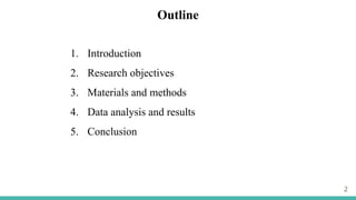
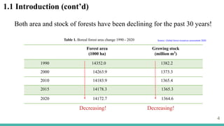
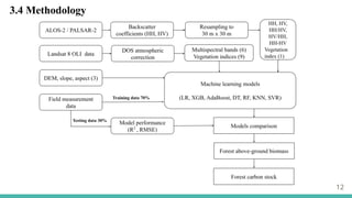
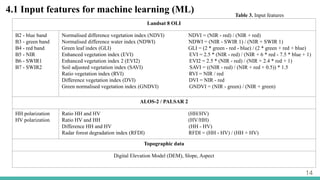
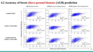
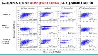
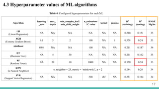
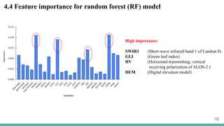
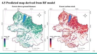
1. 1
Student: Geserbaatar
Nandin-erdene
Supervisor: Prof. Kenlo
Nishida Nasahara
16th
March, 2022
Estimation of the Above-ground Biomass
and Carbon Stock in Boreal Forest Using
Satellite Data with Machine Learning

2. Outline
1. Introduction
2. Research objectives
3. Materials and methods
4. Data analysis and results
5. Conclusion
2

3. 1. Introduction
3
Source: National Forest Inventory of Mongolia & Forest loss (Hansen et al., 2013 )
Boreal forest covers
about 9.2% of the total
area of Mongolia.
But those forests are
decreasing.
2020
2001

4. Forest area
(1000 ha)
Growing stock
(million m3
)
1990 14352.0 1382.2
2000 14263.9 1373.3
2010 14183.9 1365.4
2015 14178.3 1365.3
2020 14172.7 1364.6
Source: Global forest resources assessment 2020
4
Table 1. Boreal forest area change 1990 - 2020
Both area and stock of forests have been declining for the past 30 years!
Decreasing! Decreasing!
1.1 Introduction (cont’d)

5. 5
Forest loss is mostly due to
fire and insects!!
1.2 Introduction (cont’d) Forest loss
Forest fire and insect damages

6. 1.3 Introduction (cont’d)
6
Current situation of forest data in Mongolia
--- Have to be updated every 5 years in all forested area
--- Use field measurement and allometric equation
--- Spend more time, challenging to reach some area, and costly

7. 2. Research objectives
Main objective:
To map forest above-ground biomass and carbon stock using satellite data with
machine learning
Goals:
➢ To develop a suitable model
➢ To estimate forest above-ground biomass (AGB)
➢ To evaluate boreal forest carbon stock
7

8. 8
3. Materials and Methods
3.1 Study area
3.2 Field data
3.3 Satellite data
3.4 Methodology

9. 3.1 Study area
9
Location: Latitude: 47°N - 53°N,
Longitude: 96° E - 104°E
Climate: Average annual rainfall
270 mm, and annual mean
temperature around 1.3 °C
Climate classification: Dwc
(continental, dry winter, cold
summer)
Total area: 20466182 ha
Forested area: 9380532 ha (45.8%)
Source: Environmental information center (www.eic.mn )

10. 10
3.2 Field data
The distribution of field data
Plot arrangement
Total field plots in study area = 5720
AGB (Mg/ha) 1 - 50 50 - 100 100 - 150 150 - 200 200 - 250
Number of plot 1952 2570 1017 170 11
Average AGB (Mg/ha) 69.7
Number of plots
r = 6m DBH 6 cm - 14.9 cm
r = 12m DBH 15 cm - 29.9 cm
r = 20m DBH ≥ 30 cm
Note: Diameter breast height (DBH)
Source: Multi-purpose national forest inventory, Forest Resource Development Center

11. 3.3 Satellite data
11
Satellite name Part / Row Time
Landsat 8 OLI
p133r25, p133r27
p133r26
p134r25, p134r26, p134r27
p135r24, p135r25, p135r26, p135r27
p136r24, p136r25, p136r26, p136r27
p137r24
p137r25
p137r26
p138r25, p138r26
2014 September 10
2013 September 7
2014 September 1
2013 September 5
2019 August 28
2017 August 29
2020 September 6
2015 July 23
2018 September 8
ALOS-2 / PALSAR 2
N47E100, 101, 102
N48E098, 099, 100, 101, 102, 103, 104
N49E098, 099, 100, 101, 102, 103, 104
N50E096, 097, 098, 099,100, 101, 102, 103, 104
N51E097, 098, 099, 100, 101, 102, 103, 104
N52E097, 098, 099, 100, 101, 102
N53E098, 099
2015
Table 2. Collected satellites data

12. 12
3.4 Methodology

13. 13
4. Data analysis and results
4.1 Input features for machine learning (ML)
4.2 Accuracy of forest above-ground biomass (AGB) prediction
4.3 Hyperparameter values of ML algorithms
4.4 Feature importance for random forest (RF)
4.5 Predicted map derived from RF model
4.6 Reference data errors

14. 14
4.1 Input features for machine learning (ML)
Landsat 8 OLI
B2 - blue band
B3 - green band
B4 - red band
B5 - NIR
B6 - SWIR1
B7 - SWIR2
Normalised difference vegetation index (NDVI) NDVI = (NIR - red) / (NIR + red)
Normalised difference water index (NDWI) NDWI = (NIR - SWIR 1) / (NIR + SWIR 1)
Green leaf index (GLI) GLI = (2 * green - red - blue) / (2 * green + red + blue)
Enhanced vegetation index (EVI) EVI = 2.5 * (NIR - red) / (NIR + 6 * red - 7.5 * blue + 1)
Enhanced vegetation index 2 (EVI2) EVI2 = 2.5 * (NIR - red) / (NIR + 2.4 * red + 1)
Soil adjusted vegetation index (SAVI) SAVI = ((NIR - red) / (NIR + red + 0.5)) * 1.5
Ratio vegetation index (RVI) RVI = NIR / red
Difference vegetation index (DVI) DVI = NIR - red
Green normalised vegetation index (GNDVI) GNDVI = (NIR - green) / (NIR + green)
ALOS-2 / PALSAR 2
HH polarization
HV polarization
Ratio HH and HV (HH/HV)
Ratio HV and HH (HV/HH)
Difference HH and HV (HH - HV)
Radar forest degradation index (RFDI) RFDI = (HH - HV) / (HH + HV)
Topographic data
Digital Elevation Model (DEM), Slope, Aspect
Table 3. Input features

15. 15
4.2 Accuracy of forest above-ground biomass (AGB) prediction
RF (Random Forest) XGB (Extreme Gradient Boost) SVR (Support Vector Regression)
Landsat 8 OLI
ALOS-2 / PALSAR-2
Landsat 8 OLI &
ALOS-2 / PALSAR-2
Predicted
AGB
(Mg/ha)
Observed AGB (Mg/ha)
R2
: 0.235
RMSE : 33 Mg/ha
R2
: 0.106
RMSE : 36 Mg/ha
R2
: 0.24
RMSE : 33 Mg/ha
R2
: 0.234
RMSE : 33 Mg/ha
R2
: 0.085
RMSE : 37 Mg/ha
R2
: 0.24
RMSE : 33 Mg/ha
R2
: 0.204
RMSE : 34 Mg/ha
R2
: 0.072
RMSE : 37 Mg/ha
R2
: 0.194
RMSE : 34 Mg/ha

16. 16
4.2 Accuracy of forest above-ground biomass (AGB) prediction (cont’d)
LR (Linear Regression) AdaBoost DT (Decision Tree) KNN (k-Nearest Neighbor)
Landsat 8 OLI
ALOS-2 /
PALSAR-2
Landsat 8 OLI
& ALOS-2 /
PALSAR-2
Predicted
AGB
(Mg/ha)
Observed AGB (Mg/ha)
R2
: 0.195
RMSE : 34 Mg/ha
R2
: 0.01
RMSE : 38 Mg/ha
R2
: 0.151
RMSE : 35 Mg/ha
R2
: 0.171
RMSE : 35 Mg/ha
R2
: 0.096
RMSE : 36 Mg/ha
R2
: 0.187
RMSE : 34 Mg/ha
R2
: 0.149
RMSE : 35 Mg/ha
R2
: 0.075
RMSE : 37 Mg/ha
R2
: 0.162
RMSE : 35 Mg/ha
R2
: 0.204
RMSE : 34 Mg/ha
R2
: 0.075
RMSE : 37 Mg/ha
R2
: 0.20
RMSE : 34 Mg/ha

17. 17
4.3 Hyperparameter values of ML algorithms
Algorithm
learning
_rate
max_
depth
min_samples_leaf /
min_child_weight
n_estimators
/ C value
kernel gamma
R2
(training)
R2
(testing)
RMSE
Mg/ha
LR
(Linear Regression)
NA NA NA NA NA NA 0.210 0.151 35
XGB
(Extreme Gradient Boost )
0.1 5 2 100 NA 1 0.578 0.24 33
AdaBoost
0.01 NA NA 100 NA NA 0.211 0.187 34
DT
(Decision Tree )
NA 4 30 NA NA NA 0.211 0.162 35
RF
(Random Forest)
NA 20 10 1000 NA NA 0.570 0.24 33
KNN
(k-Nearest Neighbor)
n_neighbor = 25, metric = ‘minkowski’, p = 2 0.244 0.20 34
SVR
(Support Vector Regression)
NA NA NA 500 rbf NA 0.231 0.194 34
Table 4. Configured hyperparameters for each ML

18. 18
4.4 Feature importance for random forest (RF) model
High importance:
SWIR1 (Short-wave infrared band 1 of Landsat 8)
GLI (Green leaf index)
HV (Horizontal transmitting, vertical
receiving polarization of ALOS-2 )
DEM (Digital elevation model)

19. 19
4.5 Predicted map derived from RF model
Forest above-ground biomass Forest carbon stock

20. 20
4.6 Reference data errors
1. High AGB value on the sparse forest
2. Low AGB value on the dense forest
3. Plot covered by forest and non forest area
Notes: yellow number is AGB value, unit is Mg/ha, and yellow circle’s radius is 30 m.
1 2 3
Total 812 plots
Source: Bing aerial map & Google map

21. 21
5. Conclusion
* Hyperparameter values were effectively influenced by overfitting error.
* SVR, KNN, and LR models were high R2
in only using Landsat data.
* The best regression model was RF. The coefficient of determination (R2
) was 0.24 and
RMSE was 33 Mg/ha. Forest AGB was estimated 32.5 Mg/ha - 122.5 Mg/ha and forest carbon
stock was estimated 16.5 Mg C/ha - 62.5 Mg C/ha.
* The highest importance variables were SWIR1, GLI, HV and DEM for the RF model.
* After data screening, 812 plots of reference data were errors. From data screening analysis
and my research, forest AGB data of National Forest Inventory in Mongolia was bad quality.
* In the future, reference field data need validation and update.

22. 22
References
Dan, A. (2019). Multipurpose national forest inventory in Mongolia, 2014-2017-A tool to support sustainable forest
management. Geography, Environment, Sustainability, 12(3), 167-183.
Environmental information center. (2020). http://www.eic.mn
FAO. (2020). Global forest resources assessment 2020. FAO. http://www.fao.org/3/cb0031en/cb0031en.pdf
Hansen, M. C., P. V. Potapov, R. Moore, M. Hancher, S. A. Turubanova, A. Tyukavina, D. Thau, S. V. Stehman, S. J.
Goetz, T. R. Loveland, A. Kommareddy, A. Egorov, L. Chini, C. O. Justice, and J. R. G. Townshend. 2013.
“High-Resolution Global Maps of 21st-Century Forest Cover Change.” Science 342 (15 November): 850–53. Data
available online from: http://earthenginepartners.appspot.com/science-2013-global-forest.
FRDC. (2017). Multi-purpose national forest inventory in Mongolia
Nachin, B., & Sukhbaatar, G. (2013). Some results of forest carbon stock calculation in northern Mongolia. UNREDD.
www.unredd.net

23. Thank you for your attention!
23