Dr. Lee's Deep Learning notes

1. Deep Learning for
Computer Vision
Graham Taylor (University of Guelph)
Marc’Aurelio Ranzato (Facebook)
Honglak Lee (University of Michigan)
https://sites.google.com/site/deeplearningcvpr2014
CVPR 2014 Tutorial

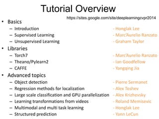
2. Tutorial Overview
• Basics
– Introduction - Honglak Lee
– Supervised Learning - Marc’Aurelio Ranzato
– Unsupervised Learning - Graham Taylor
• Libraries
– Torch7 - Marc’Aurelio Ranzato
– Theano/Pylearn2 - Ian Goodfellow
– CAFFE - Yangqing Jia
• Advanced topics
– Object detection - Pierre Sermanet
– Regression methods for localization - Alex Toshev
– Large scale classification and GPU parallelization - Alex Krizhevsky
– Learning transformations from videos - Roland Memisevic
– Multimodal and multi task learning - Honglak Lee
– Structured prediction - Yann LeCun
https://sites.google.com/site/deeplearningcvpr2014

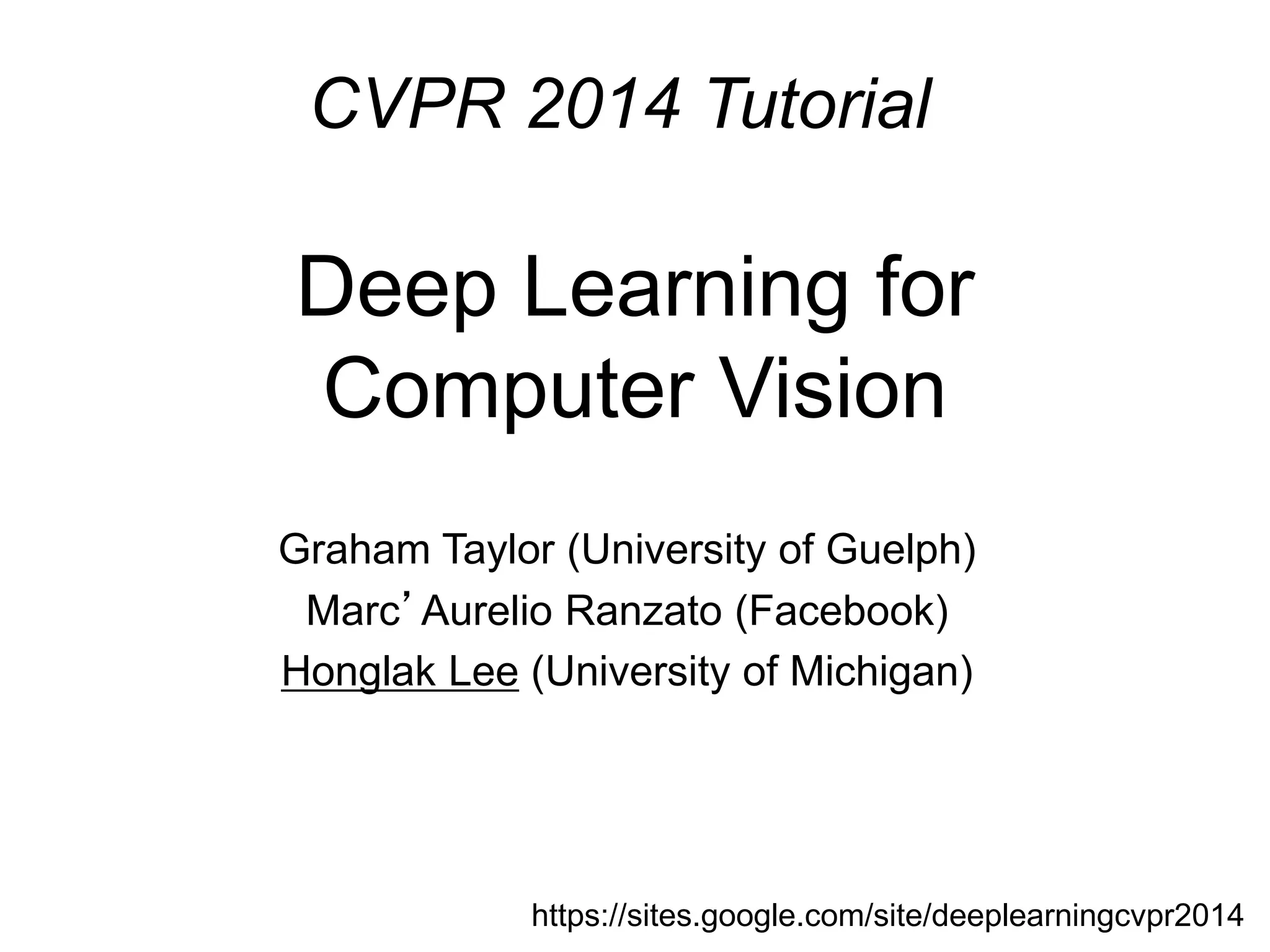
3. Image Low-level
vision features
(edges, SIFT, HOG, etc.)
Object detection
/ classification
Input data
(pixels)
Learning
Algorithm
(e.g., SVM)
feature
representation
(hand-crafted)
Features are not learned
Traditional Recognition Approach

4. SIFT Spin image
HoG
Textons
Computer vision features
SURF, MSER, LBP, Color-SIFT, Color histogram, GLOH, …..
and many others:

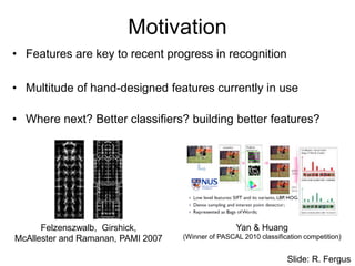
5. Motivation
• Features are key to recent progress in recognition
• Multitude of hand-designed features currently in use
• Where next? Better classifiers? building better features?
Felzenszwalb, Girshick,
McAllester and Ramanan, PAMI 2007
Yan & Huang
(Winner of PASCAL 2010 classification competition)
Slide: R. Fergus

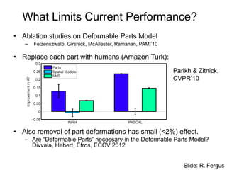
6. What Limits Current Performance?
• Ablation studies on Deformable Parts Model
– Felzenszwalb, Girshick, McAllester, Ramanan, PAMI’10
• Replace each part with humans (Amazon Turk):
• Also removal of part deformations has small (<2%) effect.
– Are “Deformable Parts” necessary in the Deformable Parts Model?
Divvala, Hebert, Efros, ECCV 2012
Parikh & Zitnick,
CVPR’10
Slide: R. Fergus

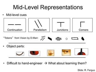
7. • Mid-level cues
Mid-Level Representations
“Tokens” from Vision by D.Marr:
Continuation Parallelism Junctions Corners
• Object parts:
• Difficult to hand-engineer  What about learning them?
Slide: R. Fergus

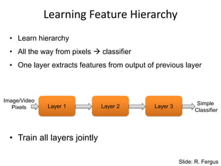
8. Learning Feature Hierarchy
• Learn hierarchy
• All the way from pixels  classifier
• One layer extracts features from output of previous layer
Layer 1 Layer 2 Layer 3
Simple
Classifier
Image/Video
Pixels
• Train all layers jointly
Slide: R. Fergus

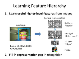
9. Learning Feature Hierarchy
1. Learn useful higher-level features from images
2. Fill in representation gap in recognition
Feature representation
Input data
1st layer
“Edges”
2nd layer
“Object parts”
3rd layer
“Objects”
Pixels
Lee et al., ICML 2009;
CACM 2011

10. Learning Feature Hierarchy
• Better performance
• Other domains (unclear how to hand engineer):
– Kinect
– Video
– Multi spectral
• Feature computation time
– Dozens of features now regularly used [e.g., MKL]
– Getting prohibitive for large datasets (10’s sec /image)
Slide: R. Fergus

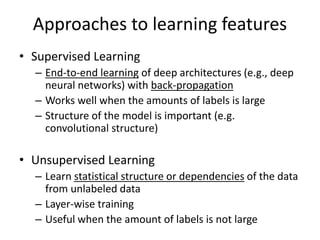
11. Approaches to learning features
• Supervised Learning
– End-to-end learning of deep architectures (e.g., deep
neural networks) with back-propagation
– Works well when the amounts of labels is large
– Structure of the model is important (e.g.
convolutional structure)
• Unsupervised Learning
– Learn statistical structure or dependencies of the data
from unlabeled data
– Layer-wise training
– Useful when the amount of labels is not large

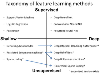
12. Taxonomy of feature learning methods
• T
• Support Vector Machine
• Logistic Regression
• Perceptron
• Deep Neural Net
• Convolutional Neural Net
• Recurrent Neural Net
• Denoising Autoencoder
• Restricted Boltzmann machines*
• Sparse coding*
• Deep (stacked) Denoising Autoencoder*
• Deep Belief Nets*
• Deep Boltzmann machines*
• Hierarchical Sparse Coding*
Deep
Shallow
Supervised
Unsupervised * supervised version exists

13. Supervised Learning

14. Example: Convolutional Neural Networks
• LeCun et al. 1989
• Neural network with
specialized connectivity
structure
Slide: R. Fergus

15. Convolutional Neural Networks
• Feed-forward:
– Convolve input
– Non-linearity (rectified linear)
– Pooling (local max)
• Supervised
• Train convolutional filters by
back-propagating classification error
Input Image
Convolution
(Learned)
Non-linearity
Pooling
LeCun et al. 1998
Feature maps
Slide: R. Fergus

16. Components of Each Layer
Pixels /
Features
Filter with
Dictionary
(convolutional
or tiled)
Spatial/Feature
(Sum or Max)
Normalization
between
feature
responses
Output
Features
+ Non-linearity
[Optional]
Slide: R. Fergus

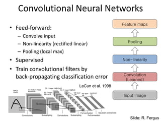
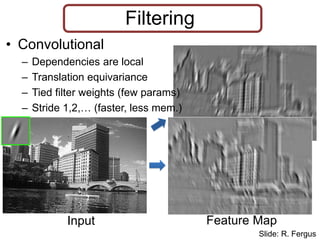
17. Filtering
• Convolutional
– Dependencies are local
– Translation equivariance
– Tied filter weights (few params)
– Stride 1,2,… (faster, less mem.)
Input Feature Map
.
.
.
Slide: R. Fergus

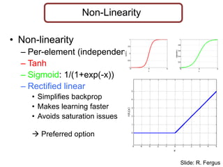
18. Non-Linearity
• Non-linearity
– Per-element (independent)
– Tanh
– Sigmoid: 1/(1+exp(-x))
– Rectified linear
• Simplifies backprop
• Makes learning faster
• Avoids saturation issues
 Preferred option
Slide: R. Fergus

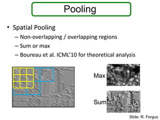
19. Pooling
• Spatial Pooling
– Non-overlapping / overlapping regions
– Sum or max
– Boureau et al. ICML’10 for theoretical analysis
Max
Sum
Slide: R. Fergus

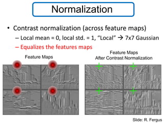
20. Normalization
• Contrast normalization (across feature maps)
– Local mean = 0, local std. = 1, “Local”  7x7 Gaussian
– Equalizes the features maps
Feature Maps
Feature Maps
After Contrast Normalization
Slide: R. Fergus

21. Compare: SIFT Descriptor
Image
Pixels Apply
Gabor filters
Spatial pool
(Sum)
Normalize to
unit length
Feature
Vector
Slide: R. Fergus

22. Applications
• Handwritten text/digits
– MNIST (0.17% error [Ciresan et al. 2011])
– Arabic & Chinese [Ciresan et al. 2012]
• Simpler recognition benchmarks
– CIFAR-10 (9.3% error [Wan et al. 2013])
– Traffic sign recognition
• 0.56% error vs 1.16% for humans [Ciresan et al. 2011]
Slide: R. Fergus

23. Application: ImageNet
Validation classification
Validation classification
Validation classification
[Deng et al. CVPR 2009]
• ~14 million labeled images, 20k classes
• Images gathered from Internet
• Human labels via Amazon Turk

24. Krizhevsky et al. [NIPS 2012]
• 7 hidden layers, 650,000 neurons, 60,000,000 parameters
• Trained on 2 GPUs for a week
• Same model as LeCun’98 but:
- Bigger model (8 layers)
- More data (106 vs 103 images)
- GPU implementation (50x speedup over CPU)
- Better regularization (DropOut)
Slide: R. Fergus

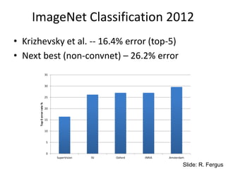
25. ImageNet Classification 2012
• Krizhevsky et al. -- 16.4% error (top-5)
• Next best (non-convnet) – 26.2% error
0
5
10
15
20
25
30
35
SuperVision ISI Oxford INRIA Amsterdam
Top-5
error
rate
%
Slide: R. Fergus

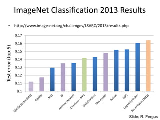
26. ImageNet Classification 2013 Results
• http://www.image-net.org/challenges/LSVRC/2013/results.php
0.1
0.11
0.12
0.13
0.14
0.15
0.16
0.17
Test
error
(top-5)
Slide: R. Fergus

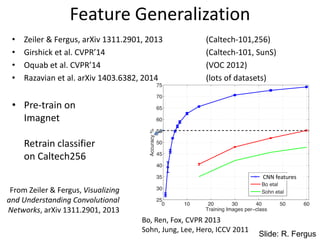
27. Feature Generalization
• Zeiler & Fergus, arXiv 1311.2901, 2013 (Caltech-101,256)
• Girshick et al. CVPR’14 (Caltech-101, SunS)
• Oquab et al. CVPR’14 (VOC 2012)
• Razavian et al. arXiv 1403.6382, 2014 (lots of datasets)
• Pre-train on
Imagnet
Retrain classifier
on Caltech256
6 training
examples
From Zeiler & Fergus, Visualizing
and Understanding Convolutional
Networks, arXiv 1311.2901, 2013
Slide: R. Fergus
CNN features
Bo, Ren, Fox, CVPR 2013
Sohn, Jung, Lee, Hero, ICCV 2011

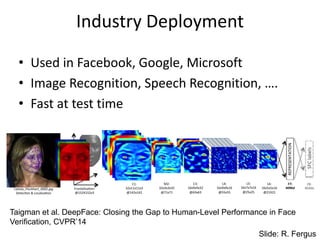
28. Industry Deployment
• Used in Facebook, Google, Microsoft
• Image Recognition, Speech Recognition, ….
• Fast at test time
Taigman et al. DeepFace: Closing the Gap to Human-Level Performance in Face
Verification, CVPR’14
Slide: R. Fergus

29. Unsupervised Learning

30. Unsupervised Learning
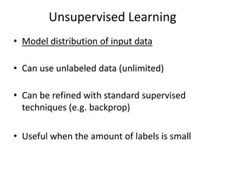
• Model distribution of input data
• Can use unlabeled data (unlimited)
• Can be refined with standard supervised
techniques (e.g. backprop)
• Useful when the amount of labels is small

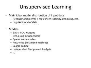
31. Unsupervised Learning
• Main idea: model distribution of input data
– Reconstruction error + regularizer (sparsity, denoising, etc.)
– Log-likelihood of data
• Models
– Basic: PCA, KMeans
– Denoising autoencoders
– Sparse autoencoders
– Restricted Boltzmann machines
– Sparse coding
– Independent Component Analysis
– …

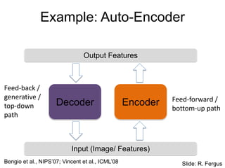
32. Example: Auto-Encoder
Encoder
Decoder
Input (Image/ Features)
Output Features
Feed-back /
generative /
top-down
path
Feed-forward /
bottom-up path
Slide: R. Fergus
Bengio et al., NIPS’07; Vincent et al., ICML’08

33. Stacked Auto-Encoders
Encoder
Decoder
Input Image
Class label
Features
Encoder
Decoder
Features
Encoder
Decoder
Slide: R. Fergus
Bengio et al., NIPS’07;
Vincent et al., ICML’08;
Ranzato et al., NIPS’07

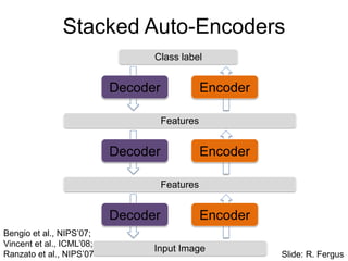
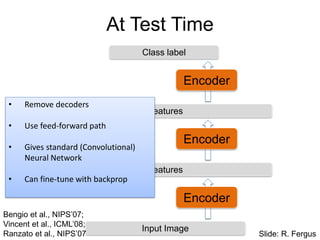
34. At Test Time
Encoder
Input Image
Class label
Features
Encoder
Features
Encoder
• Remove decoders
• Use feed-forward path
• Gives standard (Convolutional)
Neural Network
• Can fine-tune with backprop
Slide: R. Fergus
Bengio et al., NIPS’07;
Vincent et al., ICML’08;
Ranzato et al., NIPS’07

35. Natural Images Learned bases: “Edges”
50 100 150 200 250 300 350 400 450 500
50
100
150
200
250
300
350
400
450
500
50 100 150 200 250 300 350 400 450 500
50
100
150
200
250
300
350
400
450
500
50 100 150 200 250 300 350 400 450 500
50
100
150
200
250
300
350
400
450
500
~ 0.8 * + 0.3 * + 0.5 *
x ~ 0.8 * w36
+ 0.3 * w42 + 0.5 * w65
[0, 0, …, 0, 0.8, 0, …, 0, 0.3, 0, …, 0, 0.5, …]
= coefficients (feature representation)
Test example
Compact & easily
interpretable
Learning basis vectors for images
[Olshausen & Field, Nature 1996, Ranzato et al., NIPS 2007; Lee et al., NIPS 2007;
Lee et al., NIPS 2008; Jarret et al., CVPR 2009; etc.]

36. Input image (pixels)
First layer
(edges)
Higher layer
(Combinations
of edges)
Learning Feature Hierarchy
[Olshausen & Field, Nature 1996, Ranzato et al., NIPS 2007; Lee et al., NIPS 2007;
Lee et al., NIPS 2008; Jarret et al., CVPR 2009; etc.]

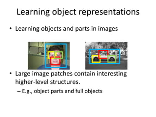
37. Learning object representations
• Learning objects and parts in images
• Large image patches contain interesting
higher-level structures.
– E.g., object parts and full objects

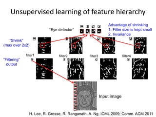
38. Input image
“Filtering”
output
“Shrink”
(max over 2x2)
filter1 filter2 filter3 filter4
“Eye detector”
Advantage of shrinking
1. Filter size is kept small
2. Invariance
Unsupervised learning of feature hierarchy
H. Lee, R. Grosse, R. Ranganath, A. Ng, ICML 2009; Comm. ACM 2011

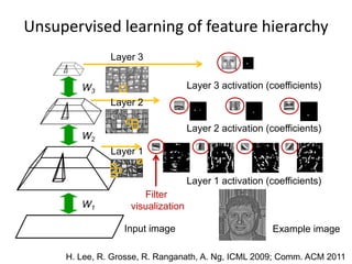
39. W1
W2
W3
Input image
Layer 1
Layer 3
Example image
Layer 1 activation (coefficients)
Layer 2 activation (coefficients)
Layer 3 activation (coefficients)
Filter
visualization
Layer 2
Unsupervised learning of feature hierarchy
H. Lee, R. Grosse, R. Ranganath, A. Ng, ICML 2009; Comm. ACM 2011

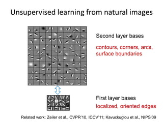
40. Unsupervised learning from natural images
First layer bases
Second layer bases
localized, oriented edges
contours, corners, arcs,
surface boundaries
Related work: Zeiler et al., CVPR’10, ICCV’11; Kavuckuglou et al., NIPS’09

41. Faces Cars Elephants Chairs
Learning object-part decomposition
Applications:
• Object recognition (Lee et al., ICML’09, Sohn et al., ICCV’11; Sohn et al., ICML’13)
• Verification (Huang et al., CVPR’12)
• Image alignment (Huang et al., NIPS’12) Cf. Convnet [Krizhevsky et al., 2012];
Deconvnet [Zeiler et al., CVPR 2010]

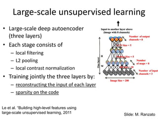
42. Large-scale unsupervised learning
• Large-scale deep autoencoder
(three layers)
• Each stage consists of
– local filtering
– L2 pooling
– local contrast normalization
• Training jointly the three layers by:
– reconstructing the input of each layer
– sparsity on the code
Le et al. “Building high-level features using
large-scale unsupervised learning, 2011 Slide: M. Ranzato

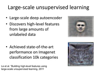
43. Large-scale unsupervised learning
• Large-scale deep autoencoder
• Discovers high-level features
from large amounts of
unlabeled data
• Achieved state-of-the-art
performance on Imagenet
classification 10k categories
Le et al. “Building high-level features using
large-scale unsupervised learning, 2011

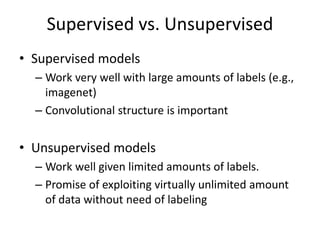
44. Supervised vs. Unsupervised
• Supervised models
– Work very well with large amounts of labels (e.g.,
imagenet)
– Convolutional structure is important
• Unsupervised models
– Work well given limited amounts of labels.
– Promise of exploiting virtually unlimited amount
of data without need of labeling

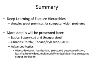
45. Summary
• Deep Learning of Feature Hierarchies
– showing great promises for computer vision problems
• More details will be presented later:
– Basics: Supervised and Unsupervised
– Libraries: Torch7, Theano/Pylearn2, CAFFE
– Advanced topics:
• Object detection, localization, structured output prediction,
learning from videos, multimodal/multitask learning, structured
output prediction

46. Tutorial Overview
• Basics
– Introduction - Honglak Lee
– Supervised Learning - Marc’Aurelio Ranzato
– Unsupervised Learning - Graham Taylor
• Libraries
– Torch7 - Marc’Aurelio Ranzato
– Theano/Pylearn2 - Ian Goodfellow
– CAFFE - Yangqing Jia
• Advanced topics
– Object detection - Pierre Sermanet
– Regression methods for localization - Alex Toshev
– Large scale classification and GPU parallelization - Alex Krizhevsky
– Learning transformations from videos - Roland Memisevic
– Multimodal and multi task learning - Honglak Lee
– Structured prediction - Yann LeCun
https://sites.google.com/site/deeplearningcvpr2014