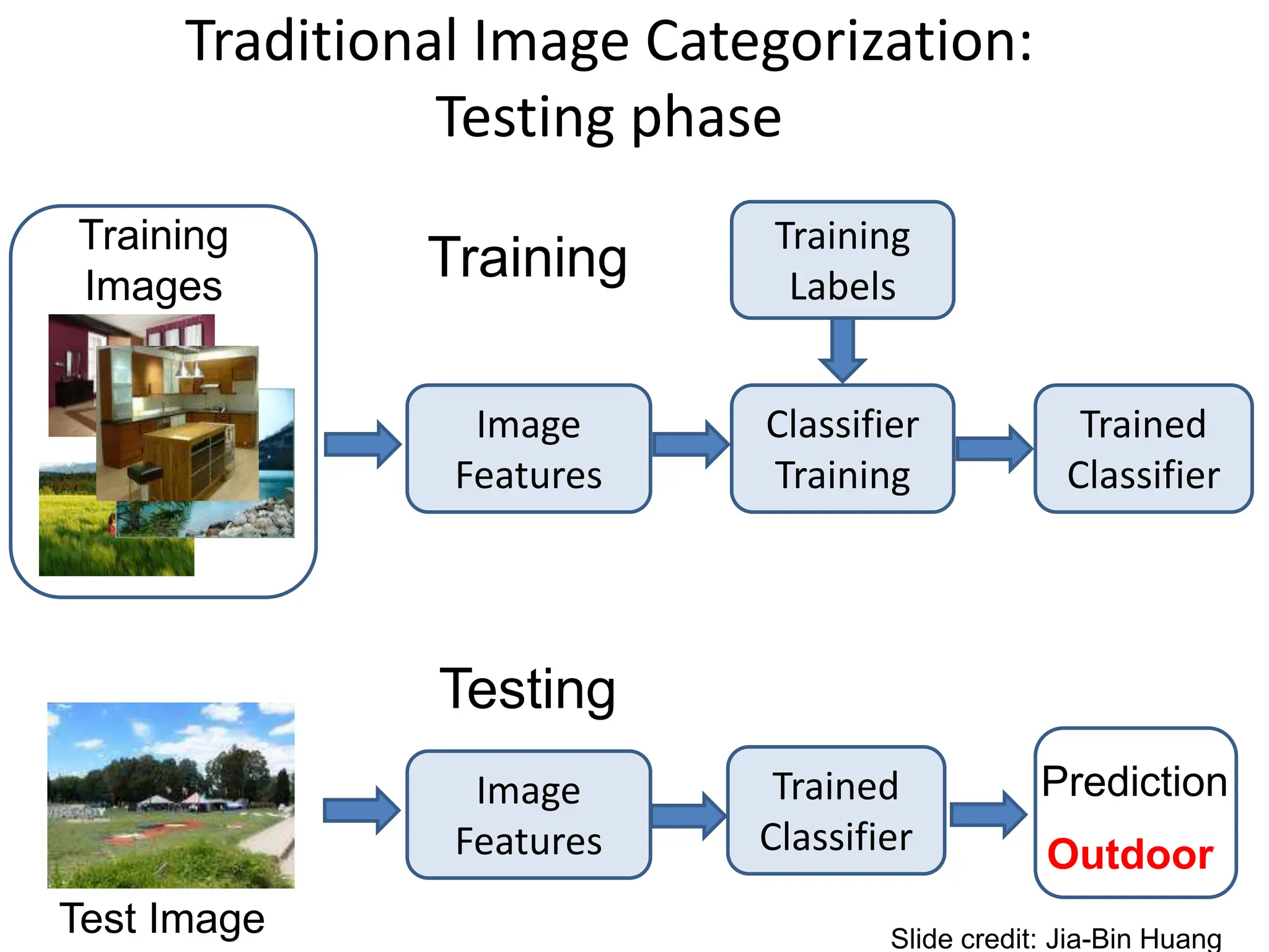
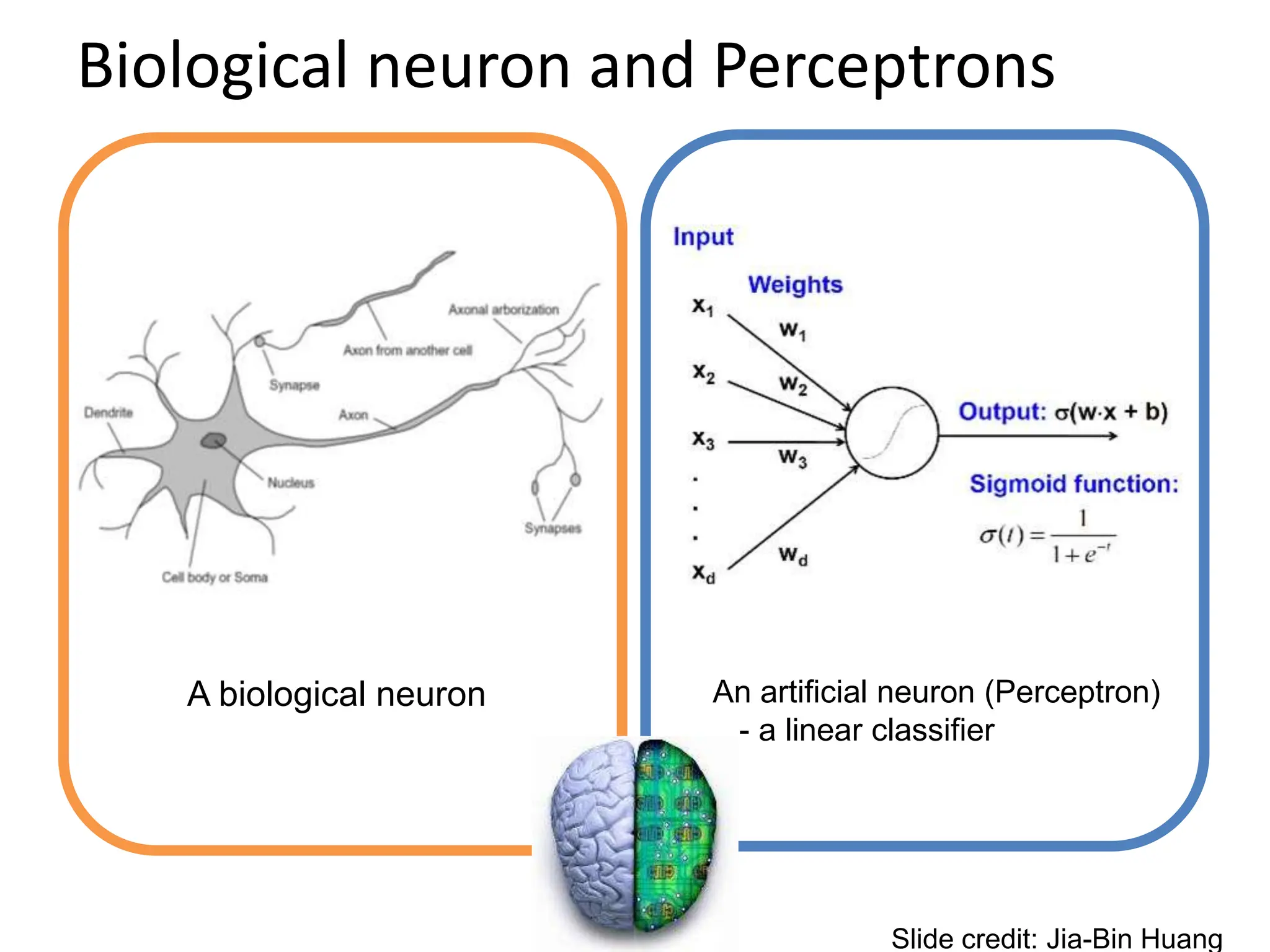
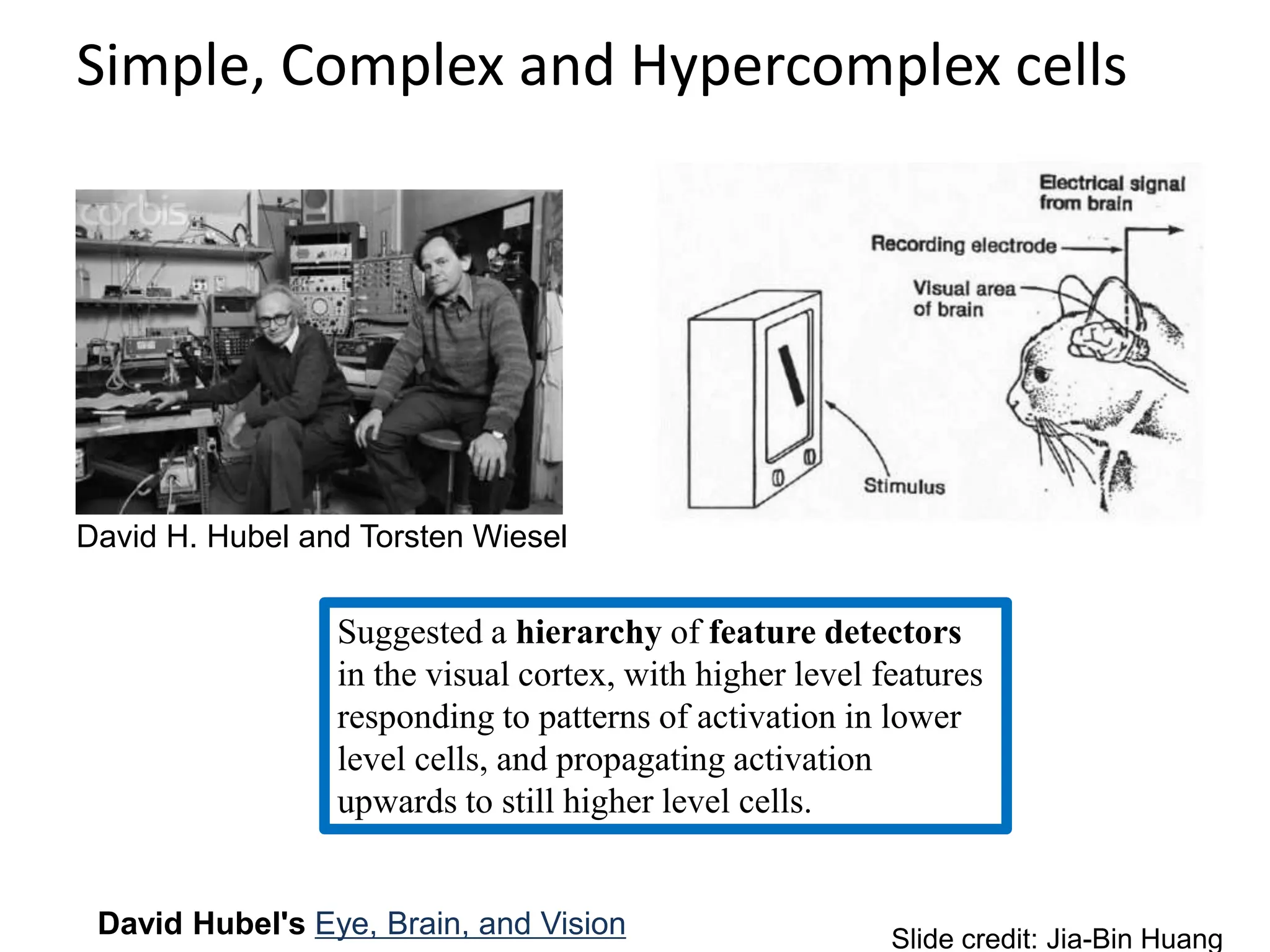
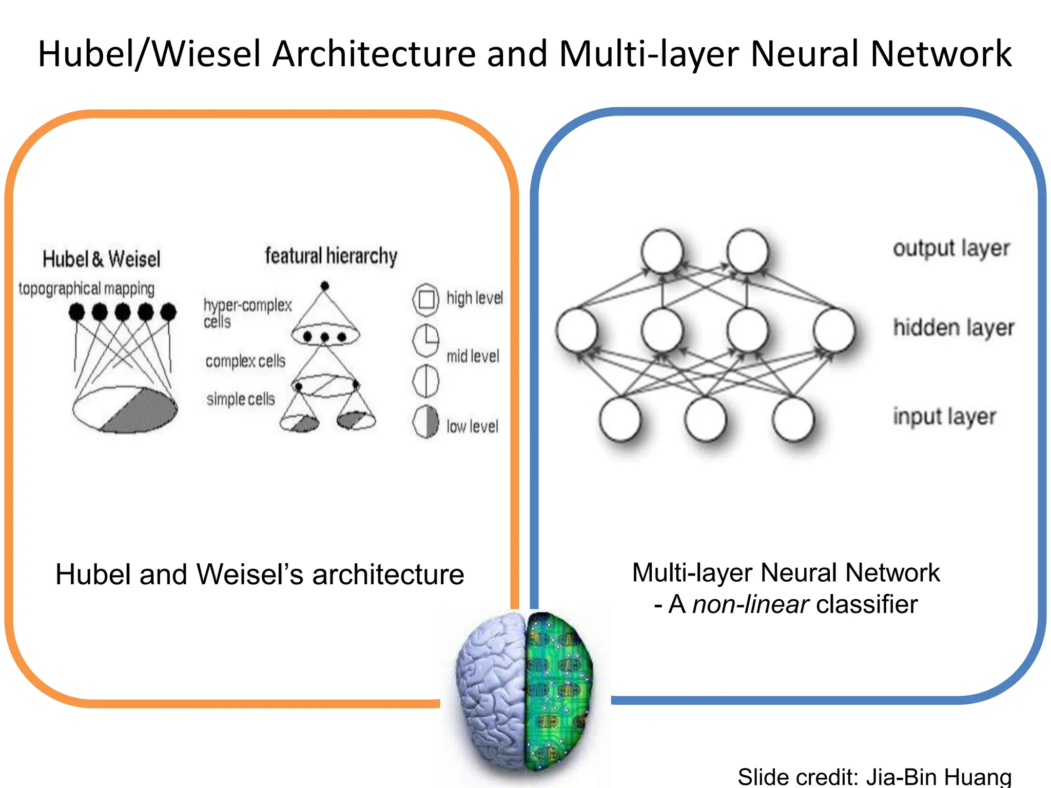
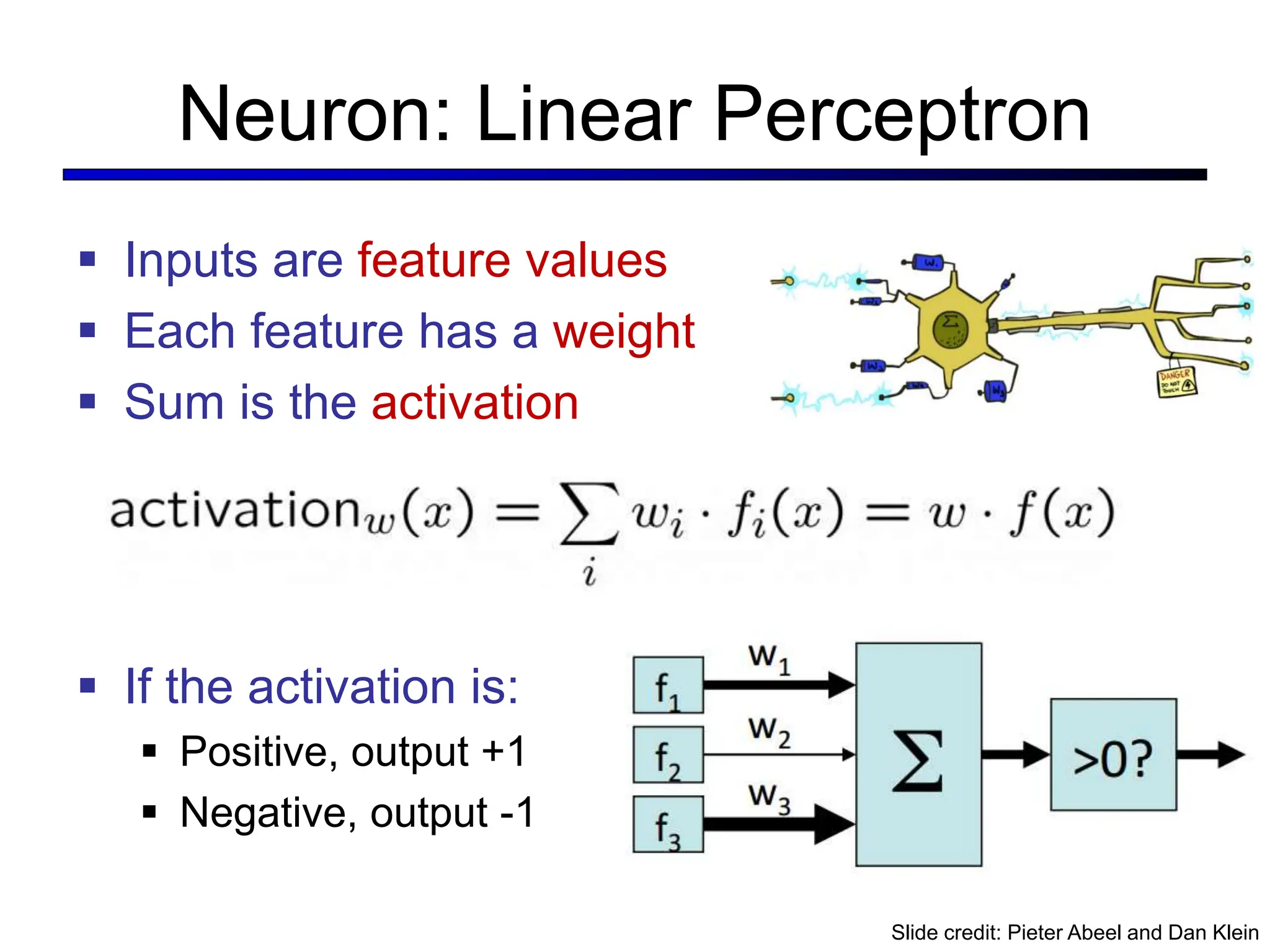
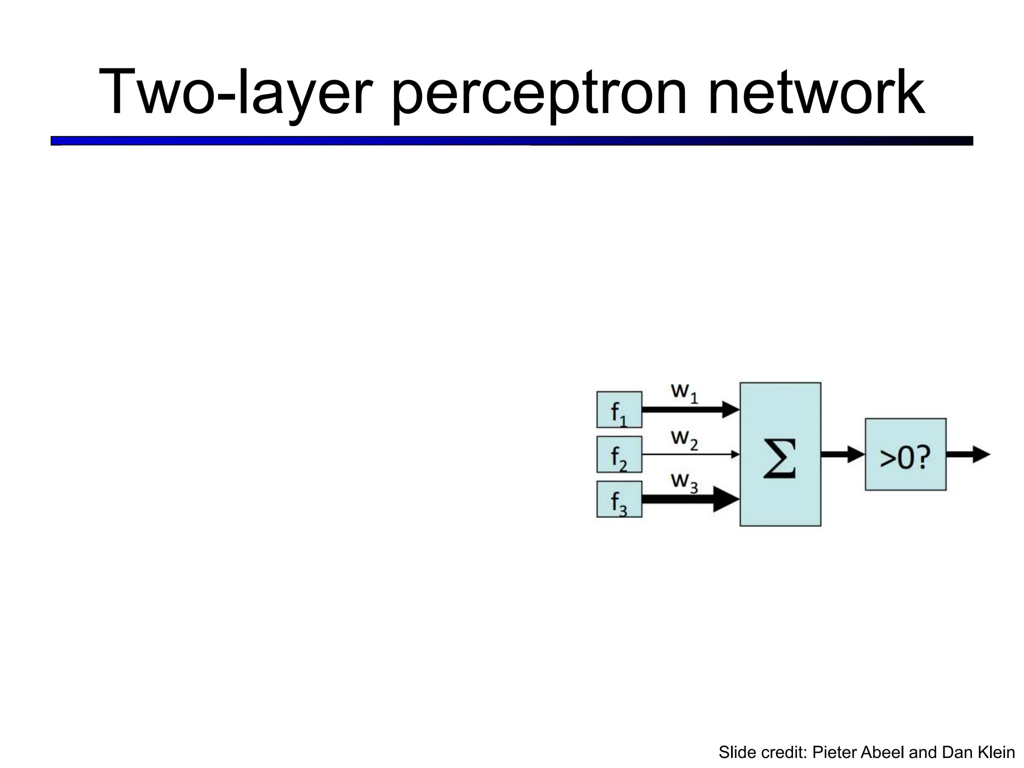
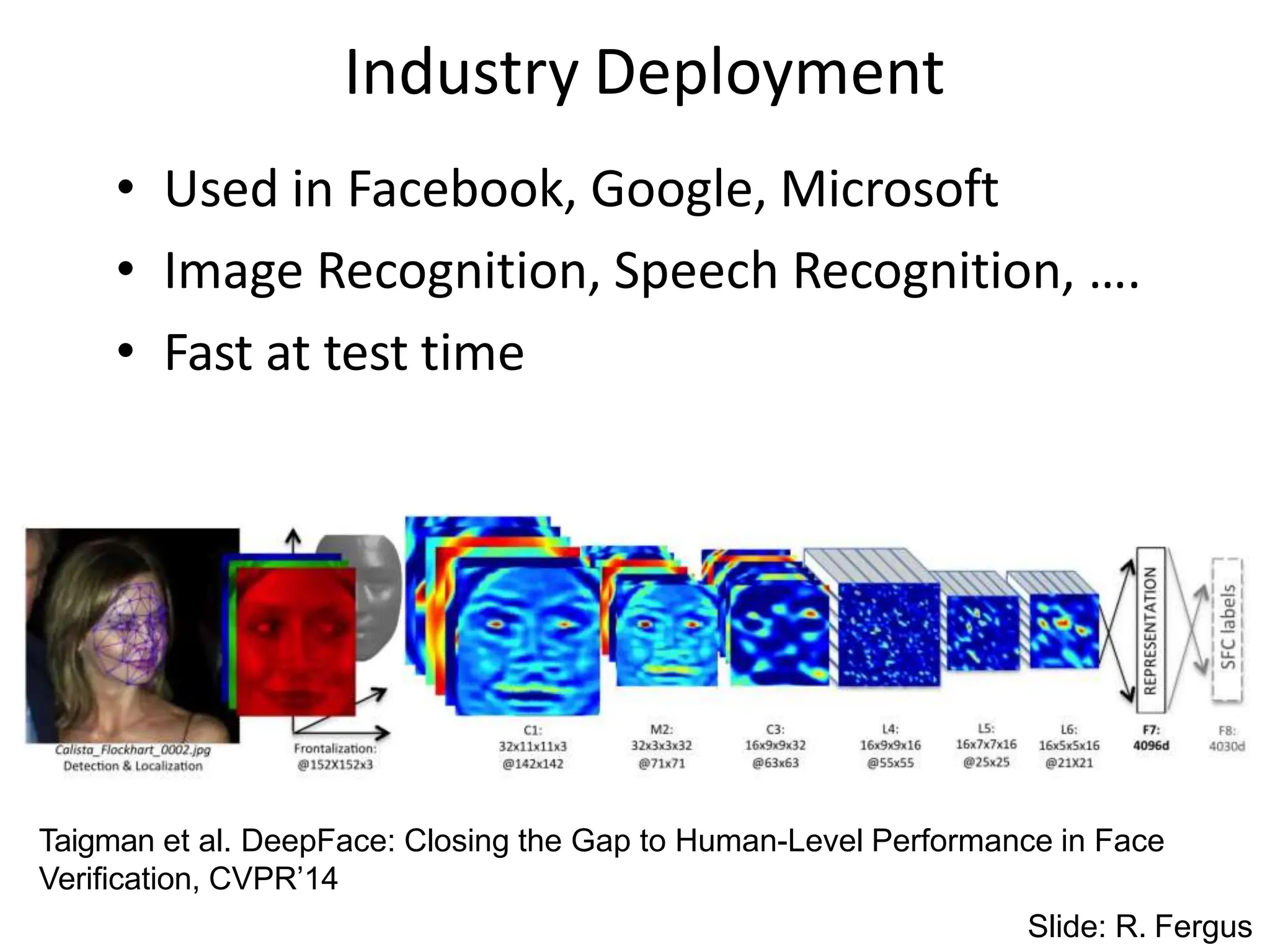
The document covers advancements in deep learning for visual recognition, particularly focusing on kernels, spatial matching techniques, and convolutional neural networks (CNNs). It discusses various feature extraction methods and the hierarchical approach to learning features from images, culminating in the success of CNNs in image classification tasks. Key implementations, such as AlexNet, are highlighted for their impact in the industry and significant performance improvements using deep learning frameworks.

1. Tues April 23
Kristen Grauman
UT Austin
Deep learning for visual
recognition

2. Last time
• Supervised classification continued
• Nearest neighbors
• Support vector machines
• HoG pedestrians example
• Kernels
• Multi-class from binary classifiers

3. Recalll: Examples of kernel functions
 Linear:
 Gaussian RBF:
 Histogram intersection:
)
2
exp(
)
( 2
2

j
i
j
i
x
x
,x
x
K





k
j
i
j
i k
x
k
x
x
x
K ))
(
),
(
min(
)
,
(
j
T
i
j
i x
x
x
x
K 
)
,
(
• Kernels go beyond vector space data
• Kernels also exist for “structured” input spaces like
sets, graphs, trees…

4. Discriminative classification with
sets of features?
• Each instance is unordered set of vectors
• Varying number of vectors per instance
Slide credit: Kristen Grauman

5. Partially matching sets of features
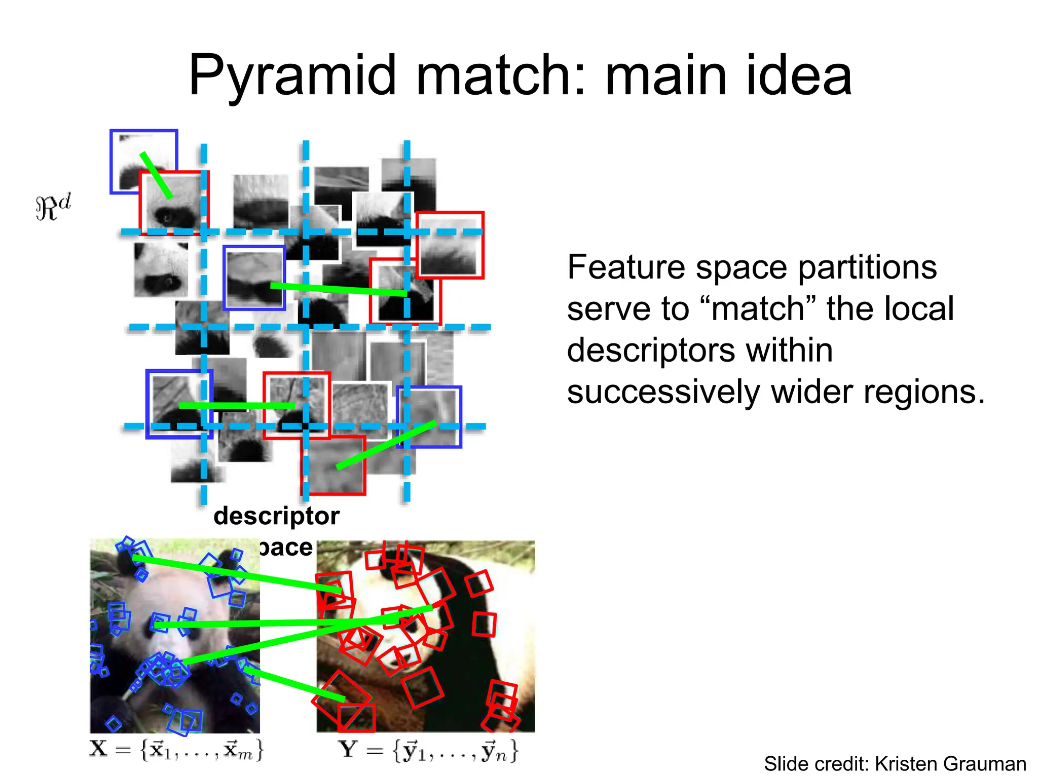
We introduce an approximate matching kernel that
makes it practical to compare large sets of features
based on their partial correspondences.
Optimal match: O(m3)
Greedy match: O(m2 log m)
Pyramid match: O(m)
(m=num pts)
[Previous work: Indyk & Thaper, Bartal, Charikar, Agarwal &
Varadarajan, …]
Slide credit: Kristen Grauman

6. Pyramid match: main idea
descriptor
space
Feature space partitions
serve to “match” the local
descriptors within
successively wider regions.
Slide credit: Kristen Grauman

7. Pyramid match: main idea
Histogram intersection
counts number of possible
matches at a given
partitioning.
Slide credit: Kristen Grauman

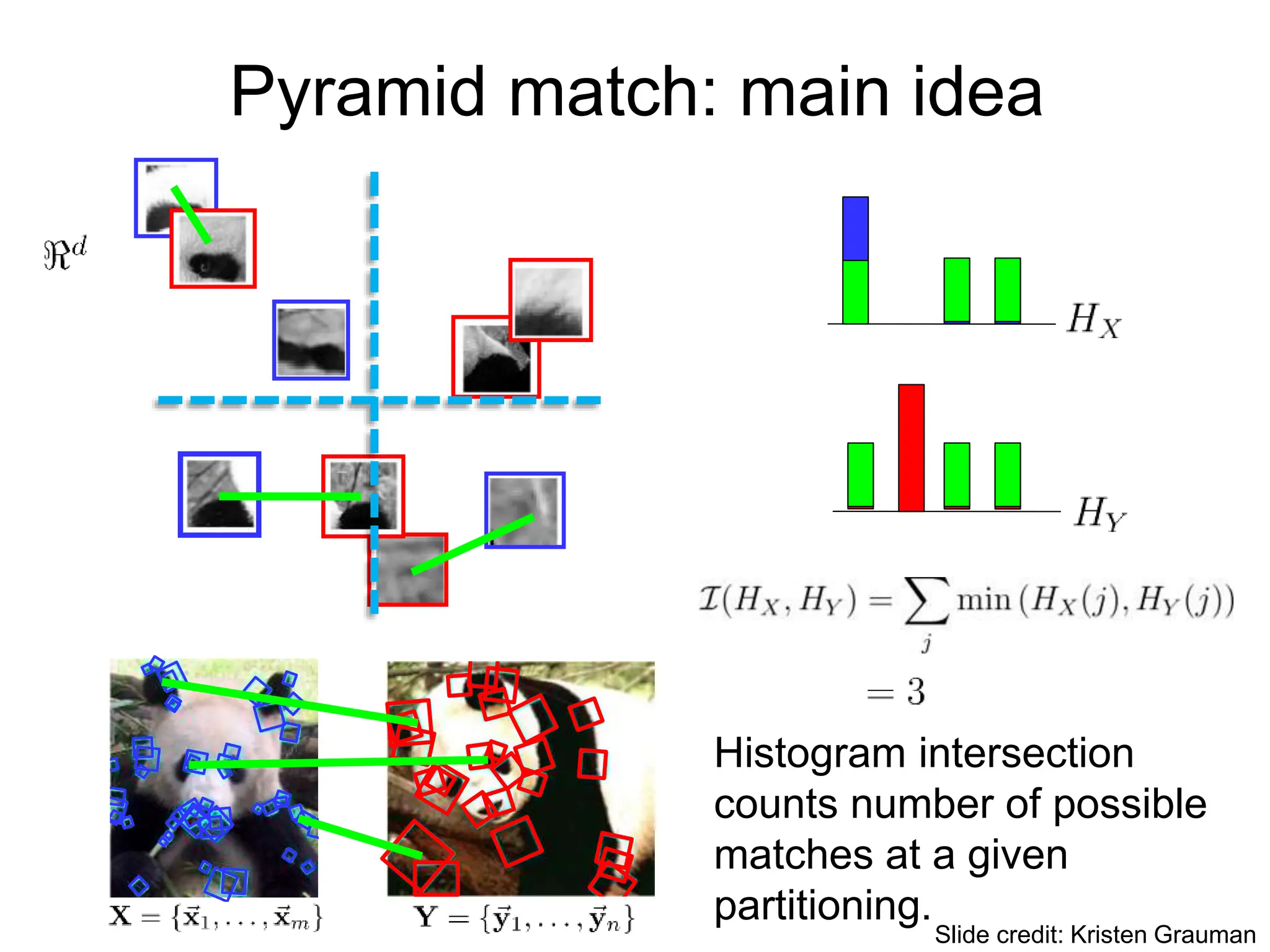
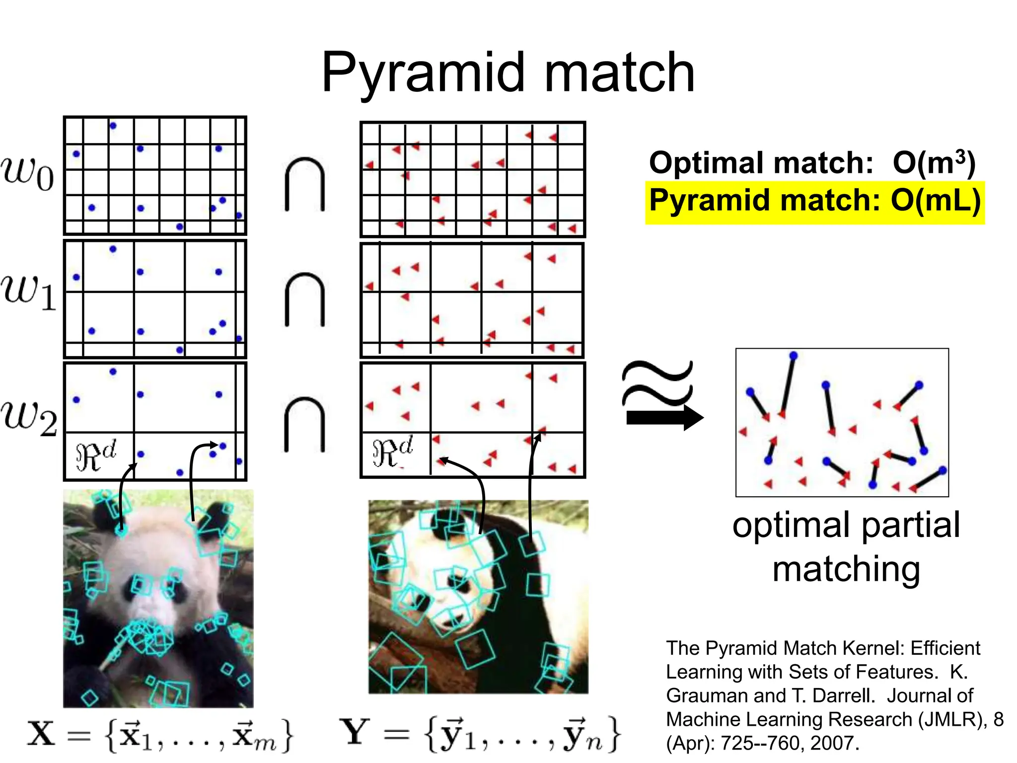
8. Pyramid match
• For similarity, weights inversely proportional to bin size
(or may be learned)
• Normalize these kernel values to avoid favoring large sets
[Grauman & Darrell, ICCV 2005]
measures
difficulty of a
match at level
number of newly matched
pairs at level
Slide credit: Kristen Grauman

9. Pyramid match
optimal partial
matching
Optimal match: O(m3)
Pyramid match: O(mL)
The Pyramid Match Kernel: Efficient
Learning with Sets of Features. K.
Grauman and T. Darrell. Journal of
Machine Learning Research (JMLR), 8
(Apr): 725--760, 2007.

10. BoW Issue:
No spatial layout preserved!
Too much? Too little?
Slide credit: Kristen Grauman

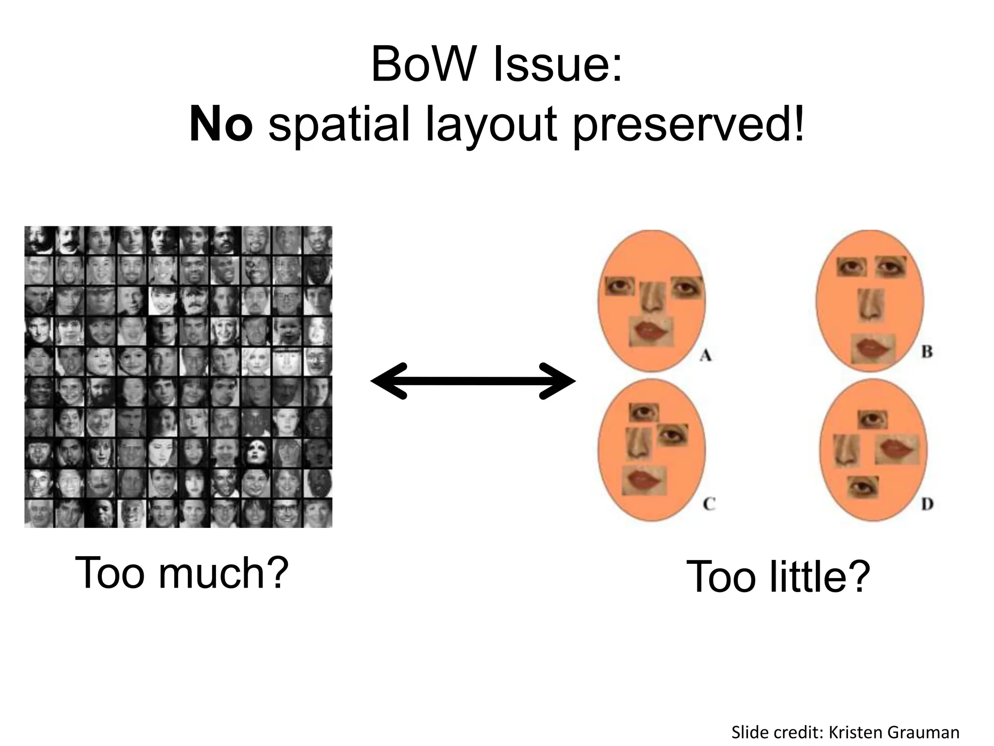
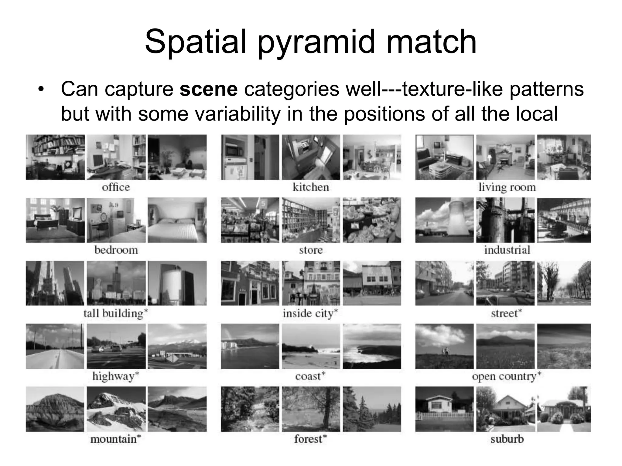
11. [Lazebnik, Schmid & Ponce, CVPR 2006]
• Make a pyramid of bag-of-words histograms.
• Provides some loose (global) spatial layout
information
Spatial pyramid match

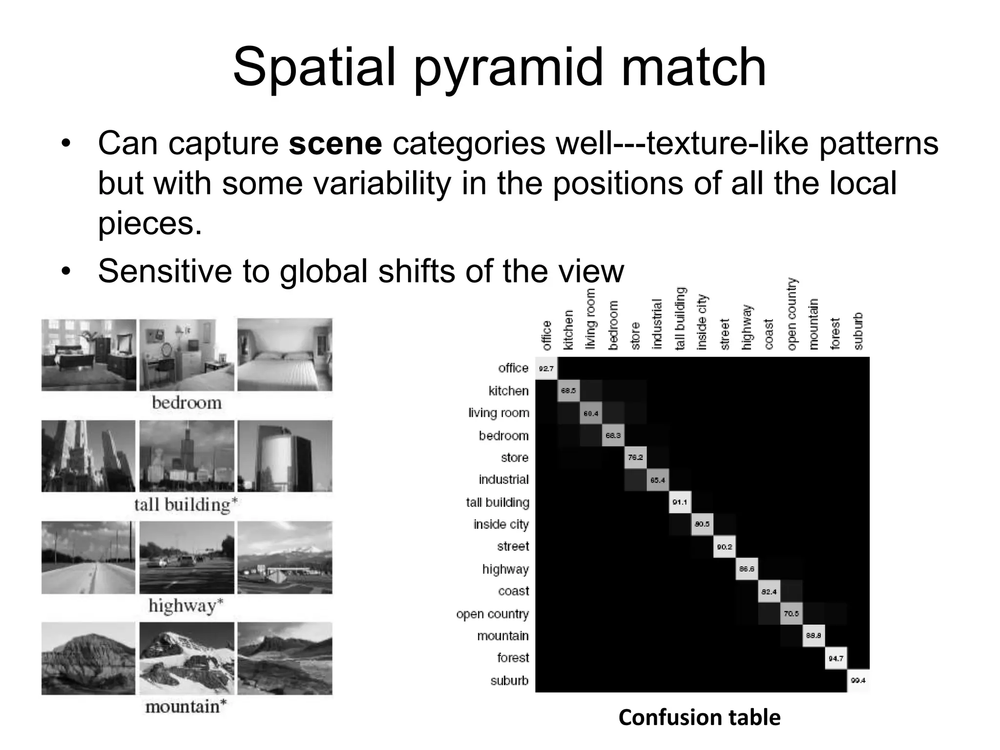
12. [Lazebnik, Schmid & Ponce, CVPR 2006]
• Make a pyramid of bag-of-words histograms.
• Provides some loose (global) spatial layout
information
Spatial pyramid match
Sum over PMKs
computed in image
coordinate space,
one per word.

13. • Can capture scene categories well---texture-like patterns
but with some variability in the positions of all the local
pieces.
Spatial pyramid match

14. • Can capture scene categories well---texture-like patterns
but with some variability in the positions of all the local
pieces.
• Sensitive to global shifts of the view
Confusion table
Spatial pyramid match

15. Today
• (Deep) Neural networks
• Convolutional neural networks

16. Traditional Image Categorization:
Training phase
Training
Labels
Training
Images
Classifier
Training
Training
Image
Features
Trained
Classifier
Slide credit: Jia-Bin Huang

17. Training
Labels
Training
Images
Classifier
Training
Training
Image
Features
Trained
Classifier
Image
Features
Testing
Test Image
Outdoor
Prediction
Trained
Classifier
Traditional Image Categorization:
Testing phase
Slide credit: Jia-Bin Huang

18. Features have been key
SIFT [Lowe IJCV 04] HOG [Dalal and Triggs CVPR 05]
SPM [Lazebnik et al. CVPR 06] Textons
SURF, MSER, LBP, Color-SIFT, Color histogram, GLOH, …..
and many others:

19. • Each layer of hierarchy extracts features from output
of previous layer
• All the way from pixels  classifier
• Layers have the (nearly) same structure
• Train all layers jointly
Learning a Hierarchy of Feature Extractors
Layer 1 Layer 2 Layer 3 Simple
Classifie
Image/Video
Pixels
Image/video Labels
Slide: Rob Fergus

20. Learning Feature Hierarchy
Goal: Learn useful higher-level features from images
Feature representation
Input data
1st layer
“Edges”
2nd layer
“Object parts”
3rd layer
“Objects”
Pixels
Lee et al., ICML2009;
CACM 2011
Slide: Rob Fergus

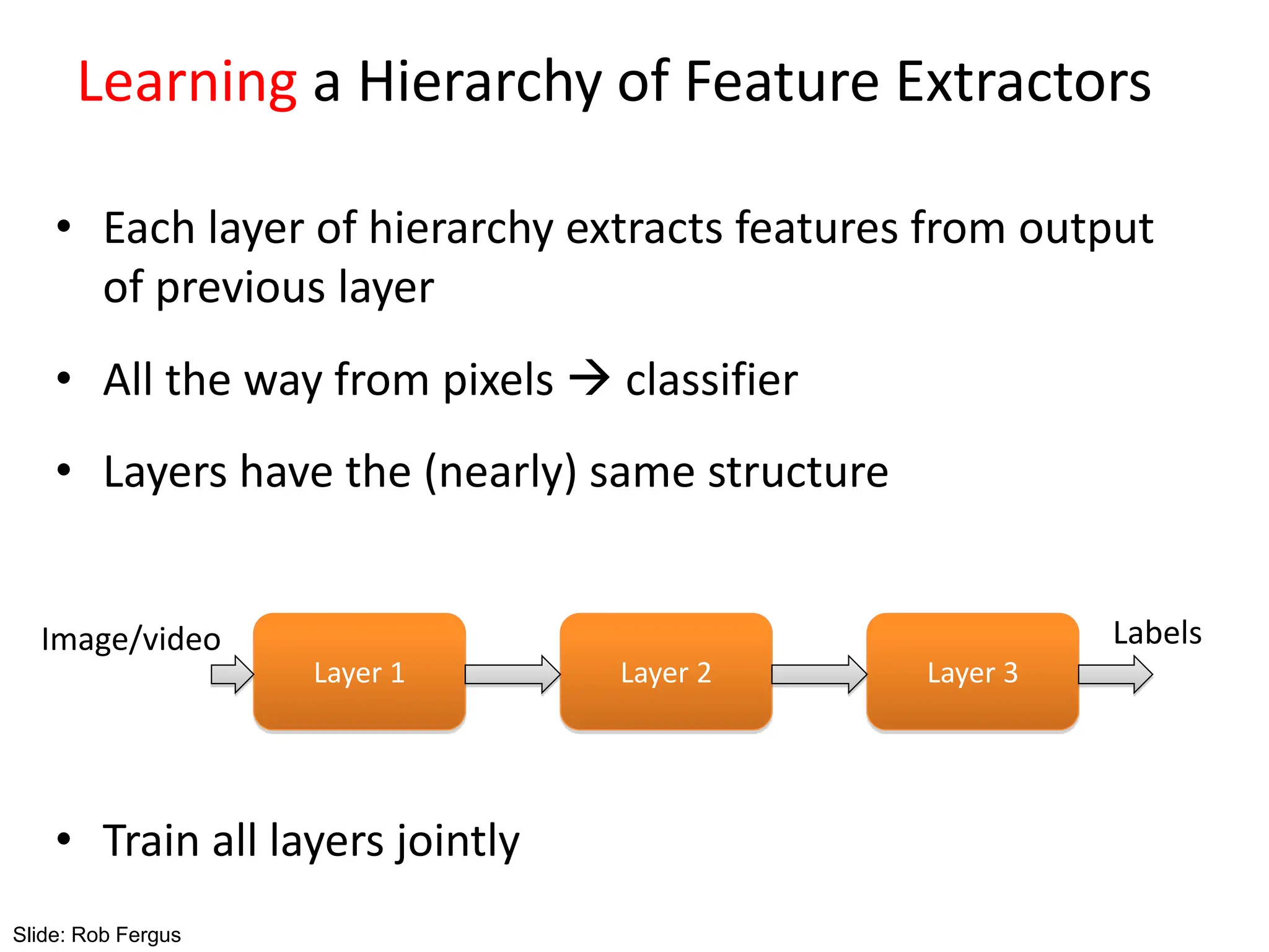
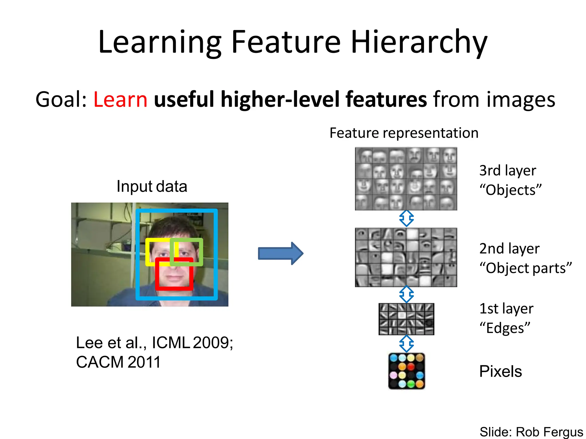
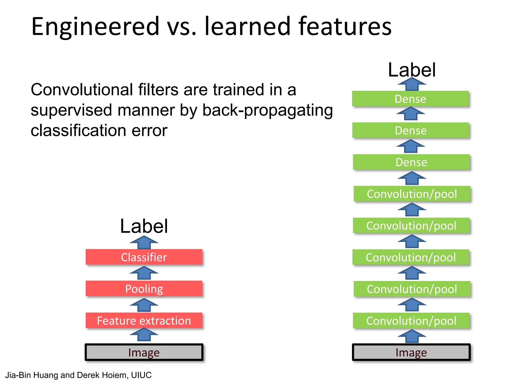
21. Learning Feature Hierarchy
• Better performance
• Other domains (unclear how to hand engineer):
– Kinect
– Video
– Multi spectral
• Feature computation time
– Dozens of features regularly used [e.g., MKL]
– Getting prohibitive for large datasets (10’s sec /image)
Slide: R. Fergus

22. Biological neuron and Perceptrons
A biological neuron An artificial neuron (Perceptron)
- a linear classifier
Slide credit: Jia-Bin Huang

23. Simple, Complex and Hypercomplex cells
David H. Hubel and Torsten Wiesel
David Hubel's Eye, Brain, and Vision
Suggested a hierarchy of feature detectors
in the visual cortex, with higher level features
responding to patterns of activation in lower
level cells, and propagating activation
upwards to still higher level cells.
Slide credit: Jia-Bin Huang

24. Hubel/Wiesel Architecture and Multi-layer Neural Network
Hubel and Weisel’s architecture Multi-layer Neural Network
- A non-linear classifier
Slide credit: Jia-Bin Huang

25. Neuron: Linear Perceptron
 Inputs are feature values
 Each feature has a weight
 Sum is the activation
 If the activation is:
 Positive, output +1
 Negative, output -1
Slide credit: Pieter Abeel and Dan Klein

26. Two-layer perceptron network
Slide credit: Pieter Abeel and Dan Klein

27. Two-layer perceptron network
Slide credit: Pieter Abeel and Dan Klein

28. Two-layer perceptron network
Slide credit: Pieter Abeel and Dan Klein

29. Learning w
 Training examples
 Objective: a misclassification loss
 Procedure:
 Gradient descent / hill climbing
Slide credit: Pieter Abeel and Dan Klein

30. Hill climbing
 Simple, general idea:
 Start wherever
 Repeat: move to the best
neighboring state
 If no neighbors better than
current, quit
 Neighbors = small
perturbations of w
 What’s bad?
 Complete?
 Optimal?
Slide credit: Pieter Abeel and Dan Klein

31. Two-layer perceptron network
Slide credit: Pieter Abeel and Dan Klein

32. Two-layer perceptron network
Slide credit: Pieter Abeel and Dan Klein

33. Two-layer neural network
Slide credit: Pieter Abeel and Dan Klein

34. Neural network properties
 Theorem (Universal function approximators): A
two-layer network with a sufficient number of
neurons can approximate any continuous
function to any desired accuracy
 Practical considerations:
 Can be seen as learning the features
 Large number of neurons
 Danger for overfitting
 Hill-climbing procedure can get stuck in bad local
optima
Slide credit: Pieter Abeel and Dan Klein
Approximation by Superpositions of Sigmoidal Function,1989

35. Today
• (Deep) Neural networks
• Convolutional neural networks

36. Significant recent impact on the field
Big labeled
datasets
Deep learning
GPU technology
0
5
10
15
20
25
30
1 2 3 4 5 6
ImageNet top-5 error (%)
Slide credit: Dinesh Jayaraman

37. Convolutional Neural Networks
(CNN, ConvNet, DCN)
• CNN = a multi-layer neural network with
– Local connectivity:
• Neurons in a layer are only connected to a small region
of the layer before it
– Share weight parameters across spatial positions:
• Learning shift-invariant filter kernels
Image credit: A. Karpathy
Jia-Bin Huang and Derek Hoiem, UIUC

38. LeNet [LeCun et al. 1998]
Gradient-based learning applied to document
recognition [LeCun, Bottou, Bengio, Haffner 1998] LeNet-1 from 1993
Jia-Bin Huang and Derek Hoiem, UIUC

39. What is a Convolution?
• Weighted moving sum
Input Feature Activation Map
.
.
.
slide credit: S. Lazebnik

40. Input Image
Convolution
(Learned)
Non-linearity
Spatial pooling
Normalization
Convolutional Neural Networks
Feature maps
slide credit: S. Lazebnik

41. Input Image
Convolution
(Learned)
Non-linearity
Spatial pooling
Normalization
Feature maps
Input Feature Map
.
.
.
Convolutional Neural Networks
slide credit: S. Lazebnik

42. Input Image
Convolution
(Learned)
Non-linearity
Spatial pooling
Normalization
Feature maps
Convolutional Neural Networks
Rectified Linear Unit (ReLU)
slide credit: S. Lazebnik

43. Input Image
Convolution
(Learned)
Non-linearity
Spatial pooling
Normalization
Feature maps
Max pooling
Convolutional Neural Networks
slide credit: S. Lazebnik
Max-pooling: a non-linear down-sampling
Provide translation invariance

44. Input Image
Convolution
(Learned)
Non-linearity
Spatial pooling
Normalization
Feature maps
Convolutional Neural Networks
slide credit: S. Lazebnik

45. Engineered vs. learned features
Image
Feature extraction
Pooling
Classifier
Label
Image
Convolution/pool
Convolution/pool
Convolution/pool
Convolution/pool
Convolution/pool
Dense
Dense
Dense
Label
Convolutional filters are trained in a
supervised manner by back-propagating
classification error
Jia-Bin Huang and Derek Hoiem, UIUC

46. SIFT Descriptor
Image
Pixels Apply
oriented filters
Spatial pool
(Sum)
Normalize to unit
length
Feature
Vector
Lowe [IJCV 2004]
slide credit: R. Fergus

47. Spatial Pyramid Matching
SIFT
Features
Filter with
Visual Words
Multi-scale
spatial pool
(Sum)
Max
Classifier
Lazebnik,
Schmid,
Ponce
[CVPR 2006]
slide credit: R. Fergus

48. Visualizing what was learned
• What do the learned filters look like?
Typical first layer filters

49. https://www.wired.com/2012/06/google-x-neural-network/

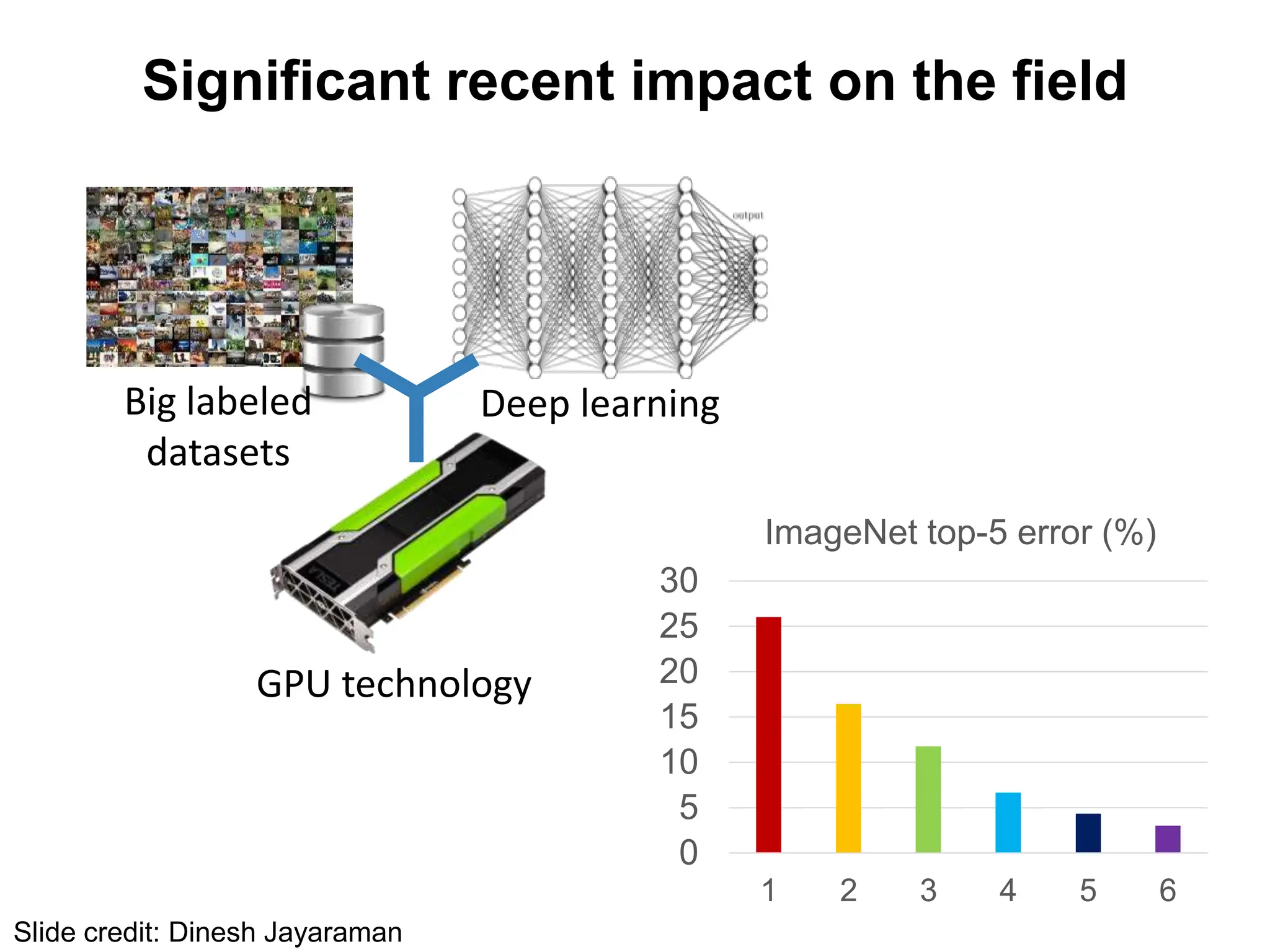
50. Application: ImageNet
[Deng et al. CVPR 2009]
• ~14 million labeled images, 20k classes
• Images gathered from Internet
• Human labels via AmazonTurk
https://sites.google.com/site/deeplearningcvpr2014 Slide: R. Fergus

51. AlexNet
• Similar framework to LeCun’98 but:
• Bigger model (7 hidden layers, 650,000 units, 60,000,000 params)
• More data (106 vs. 103 images)
• GPU implementation (50x speedup over CPU)
• Trained on two GPUs for a week
A. Krizhevsky, I. Sutskever, and G. Hinton,
ImageNet Classification with Deep Convolutional Neural Networks, NIPS 2012
Jia-Bin Huang and Derek Hoiem, UIUC

52. ImageNet Classification Challenge
http://image-net.org/challenges/talks/2016/ILSVRC2016_10_09_clsloc.pdf
AlexNet

53. Industry Deployment
• Used in Facebook, Google, Microsoft
• Image Recognition, Speech Recognition, ….
• Fast at test time
Taigman et al. DeepFace: Closing the Gap to Human-Level Performance in Face
Verification, CVPR’14
Slide: R. Fergus

54. Recap
• Neural networks / multi-layer perceptrons
– View of neural networks as learning hierarchy of
features
• Convolutional neural networks
– Architecture of network accounts for image
structure
– “End-to-end” recognition from pixels
– Together with big (labeled) data and lots of
computation  major success on benchmarks,
image classification and beyond