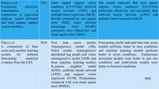
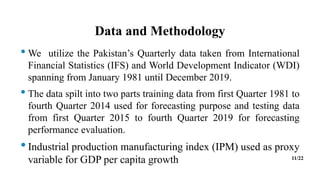
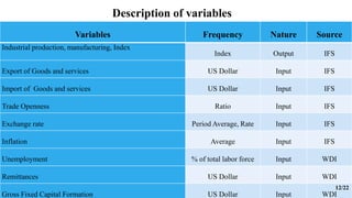
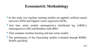
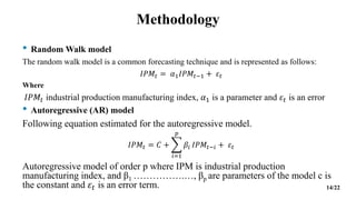
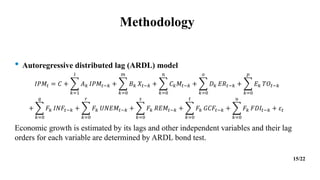
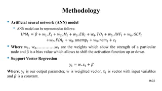
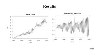
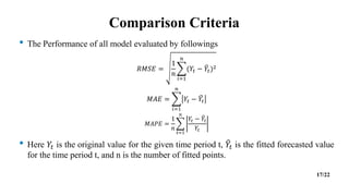
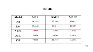
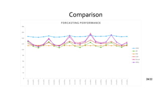
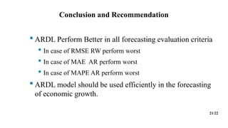
1) The document describes a study comparing time series and machine learning models for forecasting economic growth in Pakistan. 2) It uses quarterly data from 1981 to 2019 on indicators like industrial production and GDP to test autoregressive (AR), random walk (RW), autoregressive distributed lag (ARDL), artificial neural network (ANN), and support vector regression (SVR) models. 3) The results show that the ARDL model performed best overall according to error metrics like RMSE, MAE, and MAPE, and thus is recommended for efficiently forecasting economic growth.

1. 1/22

2. DEMOGRAPHIC DIVIDEND AND ECONOMIC GROWTH
NEXUS IN ASIAN COUNTRIES: PANELAUTO REGRESSIVE
APPROACH (PVAR)
By : Shazia Anwar
Supervisor : Dr. Hafsa Hina
Department of Economics & Econometrics
Pakistan Institute of Development Economics
2/22

3. Contents
• Introduction
• Objective of the Study
• Significance of the study
• Literature Review
• Data and Methodology
• Comparison Criteria
• Results
• Conclusion And Recommendation
3/22

4. Introduction
• Forecasting is a core feature of time series data.
• Forecasting refers to the practice of predicting what will happen in the
future by taking into consideration events in the past and present.
• There are many forecasting time series and machine learning models.
• Time series
oAutoregressive distributed lag (ARDL) model
oAutoregressive (AR) model
oVector auto regressive (VAR) model
oAutoregressive integrated moving average model (ARIMA)
oRandom walk (RW) model)
4/22

5. Introduction
• Machine learning
oArtificial Neural Network (ANN),
oK nearest neighbor (KNN),
oSupport vector Machine (SVM),
oSupport vector Regression (SVR)
• There are many criteria’s for forecasting evolution like root mean
square error (RMSE), mean absolute error (MAE) and mean absolute
percentage error (MAPE).
5/22

6. Introduction
•Forecasting in economic growth is an important topic.
•There are many indicators of economic growth
•Gross domestic product (GDP) per capita growth is an
imperative indicator to interrogate the growth of the country’s
economy.
6/22

7. Objectives of the study
•To make the comparison between traditional time series
and machine learning models
•To make comparison between time series and machine
learning models in case of univariate and multivariate
models
•To forecast economic growth through traditional time
series and Machine Learning models
7/22

8. Significance of The Study
•We are unable to find any study which forecast the
economic growth through machine learning models in
case of Pakistan.
•We are also unable to find any comparative study which
compare time series models and machine learning models
in case of Pakistan.
•We have tried to fill above the gaps in literature. 8/22

9. Literature Review
Author name
and article name
Years Methods name Findings
Milačić et al.
Application of
artificial neural
network with
extreme learning
machine for
economic growth
estimation
2017 Artificial Neural Network (ANN) with
extreme learning machine (ELM) and
back propagation (BP). Performance
tested with root mean square error
(RMSE), coefficient of determination
(R2) and Pearson coefficient (r).
This study concluded that the extreme
learning machine (ELM) algorithms
performed better than back propagation
(BP) algorithms.
Beyca, et al.
Using machine
learning tools for
forecasting natural
gas consumption in
the province of
Istanbul.
2019 Artificial Neural Network (ANN),
Support Vector Regression (SVR), and
Multiple Linear Regression (MLR).
Performance tested with mean absolute
percentage error (MAPE) and mean
square error (MSE).
This study indicated that support vector
regression (SVR) forecasted better than
artificial neural network (ANN) and
multiple linear regression (MLR). Yet
overall all models performed better and had
error less than 5% for estimation of real
consumption. 9/22

10. Kaytez et al.
Forecasting electricity
consumption: A
comparison of regression
analysis, neural networks
and least squares support
vector machines.
2015 Least square support vector
machines (LS-SVMs), artificial
neural network (ANN) and
multiple linear regression (MLR).
Results compared by sum square
error (SSE) mean absolute
percentage error (MAPE)
maximum error (MaxError) and
mean square error (MSE).
The results indicated that least square
support vector machines (LS-SVMs)
performed effectively and accurately than
artificial neural network (ANN) and
multiple linear regression (MLR).
Ülke et al
A comparison of time
series and machine learning
models for inflation
forecasting: empirical
evidence from the USA
2016 Four time series models
Autoregressive model (AR),
Naïve model, Autoregressive
distributed lag model and vector
autoregressive model (VAR) and
three machine learning models,
K-nearest neighbor model
(KNN), artificial neural network
(ANN) and support vector
regression (SVM). Performance
compared with root mean square
error (RMSE).
Forecasting results indicated that time series
models performs better in nine conditions
and machine learning models performs
better in seven conditions. Furthermore
univariate models were better in just two
conditions and multivariate models were
better in fourteen conditions.
10/22

11. Data and Methodology
• We utilize the Pakistan’s Quarterly data taken from International
Financial Statistics (IFS) and World Development Indicator (WDI)
spanning from January 1981 until December 2019.
• The data spilt into two parts training data from first Quarter 1981 to
fourth Quarter 2014 used for forecasting purpose and testing data
from first Quarter 2015 to fourth Quarter 2019 for forecasting
performance evaluation.
•Industrial production manufacturing index (IPM) used as proxy
variable for GDP per capita growth 11/22

12. Description of variables
Data
Data will be taken from climatic data processing center (CDPC) of
Pakistan meteorological department (PMD).
Variables Frequency Nature Source
Industrial production, manufacturing, Index
Index Output IFS
Export of Goods and services US Dollar Input IFS
Import of Goods and services US Dollar Input IFS
Trade Openness Ratio Input IFS
Exchange rate Period Average, Rate Input IFS
Inflation Average Input IFS
Unemployment % of total labor force Input WDI
Remittances US Dollar Input WDI
Gross Fixed Capital Formation US Dollar Input WDI
12/22

13. Econometric Methodology
• In this study two machine learning models are applied: artificial neural
network (ANN) and Support vector regression (SVR).
• And time series models autoregressive distributed lag (ARDL),
Autoregressive (AR) and Random walk (RW)
• Then compare machine learning and time series models
• The performance of the forecasting models evaluated through RMSE,
MAPE and MAE.
13/22

14. Methodology
• Random Walk model
The random walk model is a common forecasting technique and is represented as follows:
𝐼𝑃𝑀𝑡 = 𝛼1𝐼𝑃𝑀𝑡−1 + 𝜀𝑡
Where
𝐼𝑃𝑀𝑡 industrial production manufacturing index, 𝛼1 is a parameter and 𝜀𝑡 is an error
• Autoregressive (AR) model
Following equation estimated for the autoregressive model.
𝐼𝑃𝑀𝑡 = 𝐶 +
𝑖=1
𝑝
𝛽𝑖 𝐼𝑃𝑀𝑡−𝑖 + 𝜀𝑡
Autoregressive model of order p where IPM is industrial production
manufacturing index, and β1 …………….…, βp are parameters of the model c is
the constant and 𝜀𝑡 is an error term. 14/22

15. Methodology
• Autoregressive distributed lag (ARDL) model
𝐼𝑃𝑀𝑡 = 𝐶 +
𝑘=1
𝑙
𝐴𝑘 𝐼𝑃𝑀𝑡−𝑘 +
𝑘=0
𝑚
𝐵𝑘 𝑋𝑡−𝑘 +
𝑘=0
𝑛
𝐶𝑘𝑀𝑡−𝑘 +
𝑘=0
𝑜
𝐷𝑘 𝐸𝑅𝑡−𝑘 +
𝑘=0
𝑝
𝐸𝑘 𝑇𝑂𝑡−𝑘
+
𝑘=0
𝑞
𝐹𝑘 𝐼𝑁𝐹𝑡−𝑘 +
𝑘=0
𝑟
𝐹𝑘 𝑈𝑁𝐸𝑀𝑡−𝑘 +
𝑘=0
𝑠
𝐹𝑘 𝑅𝐸𝑀𝑡−𝑘 +
𝑘=0
𝑡
𝐹𝑘 𝐺𝐶𝐹𝑡−𝑘 +
𝑘=0
𝑢
𝐹𝑘 𝐹𝐷𝐼𝑡−𝑘 + 𝜀𝑡
Economic growth is estimated by its lags and other independent variables and their lag
orders for each variable are determined by ARDL bond test.
15/22

16. Methodology
• Artificial neural network (ANN) model
• ANN model can be represented as follows:
𝐼𝑃𝑀𝑡 = 𝛽 + 𝑤1. 𝑋𝑡 + 𝑤2. 𝑀𝑡 + 𝑤3. 𝐸𝑅𝑡 + 𝑤4. 𝑇𝑂𝑡 + 𝑤5. 𝐼𝑁𝐹𝑡 + 𝑤6. 𝐺𝐶𝐹𝑡
+𝑤7. 𝐹𝐷𝐼𝑡 + 𝑤8. 𝑢𝑛𝑒𝑚𝑝𝑡 + 𝑤9. 𝑟𝑒𝑚𝑡 + 𝜀𝑡
• Where 𝑤1, 𝑤2,…………,𝑤9 are the weights which show the strength of a particular
node and β is a bias value which allows to shift the activation function up or down.
• Support Vector Regression
𝑦𝑡 = 𝑤. 𝑥𝑡 + 𝛽
Where, 𝑦𝑡 is our output parameter, w is weighted vector, 𝑥𝑡 is vector with input variables
and 𝛽 is a constant.
16/22

17. Comparison Criteria
• The Performance of all model evaluated by followings
𝑅𝑀𝑆𝐸 =
1
𝑛
𝑖=1
𝑛
(𝑌𝑡 − 𝑌𝑡)2
𝑀𝐴𝐸 =
𝑖=1
𝑛
𝑌𝑡 − 𝑌𝑡
𝑀𝐴𝑃𝐸 =
1
𝑛
𝑡=1
𝑛
𝑌𝑡 − 𝑌𝑡
𝑌𝑡
• Here 𝑌𝑡 is the original value for the given time period t, 𝑌𝑡 is the fitted forecasted value
for the time period t, and n is the number of fitted points.
17/22

18. Results
18/22

19. Results
19/22
Model MAE RMSE MAPE
AR 14.5245 12.3863 10.6091
RW 14.0648 18.2813 10.3007
ARDL 2.1806 2.7437 1.6766
ANN 5.9474 6.4546 4.0920
SVR 7.7888 10.4769 5.6956

20. Comparison
0
20
40
60
80
100
120
140
160
180
2
0
1
5
Q
1
2
0
1
5
Q
2
2
0
1
5
Q
3
2
0
1
5
Q
4
2
0
1
6
Q
1
2
0
1
6
Q
2
2
0
1
6
Q
3
2
0
1
6
Q
4
2
0
1
7
Q
1
2
0
1
7
Q
2
2
0
1
7
Q
3
2
0
1
7
Q
4
2
0
1
8
Q
1
2
0
1
8
Q
2
2
0
1
8
Q
3
2
0
1
8
Q
4
2
0
1
9
Q
1
2
0
1
9
Q
2
2
0
1
9
Q
3
2
0
1
9
Q
4
FORCASTING PERFORMANCE
ANN
AR
RW
SVR
Actual
ARDL
20/22

21. Conclusion and Recommendation
•ARDL Perform Better in all forecasting evaluation criteria
• In case of RMSE RW perform worst
• In case of MAE AR perform worst
• In case of MAPE AR perform worst
•ARDL model should be used efficiently in the forecasting
of economic growth.
21/22

22. Thank You
22/22