Download to read offline


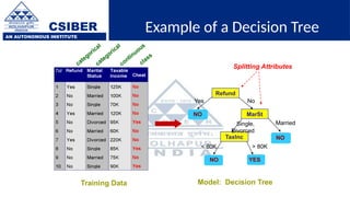
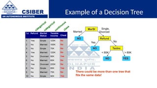
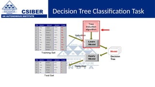
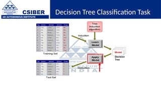
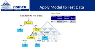
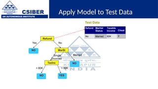
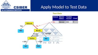
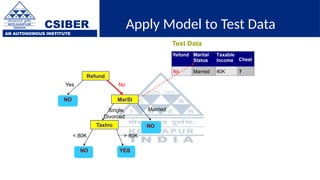
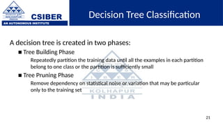
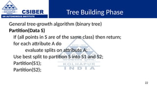
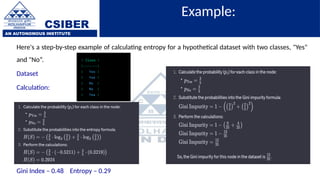
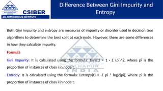
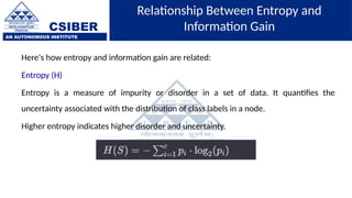
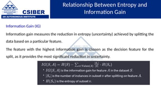


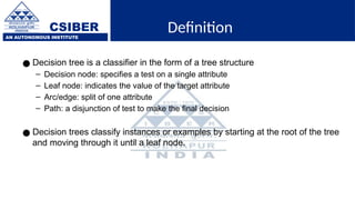

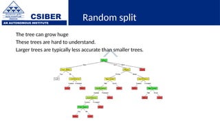
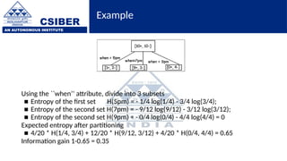


The document provides an overview of decision trees, a popular machine learning algorithm used for classification and regression tasks, highlighting their structure, building process, and key terminologies such as root nodes, branches, and leaf nodes. It discusses the advantages of decision trees, including ease of interpretation and handling of different data types, while also addressing their tendency to overfit and the importance of techniques like pruning. Additionally, the document covers the criteria for selecting attributes such as Gini impurity and entropy, emphasizing their roles in determining the best splits during the tree-building process.


