Classification algorithms in Machine Learning

1. 1
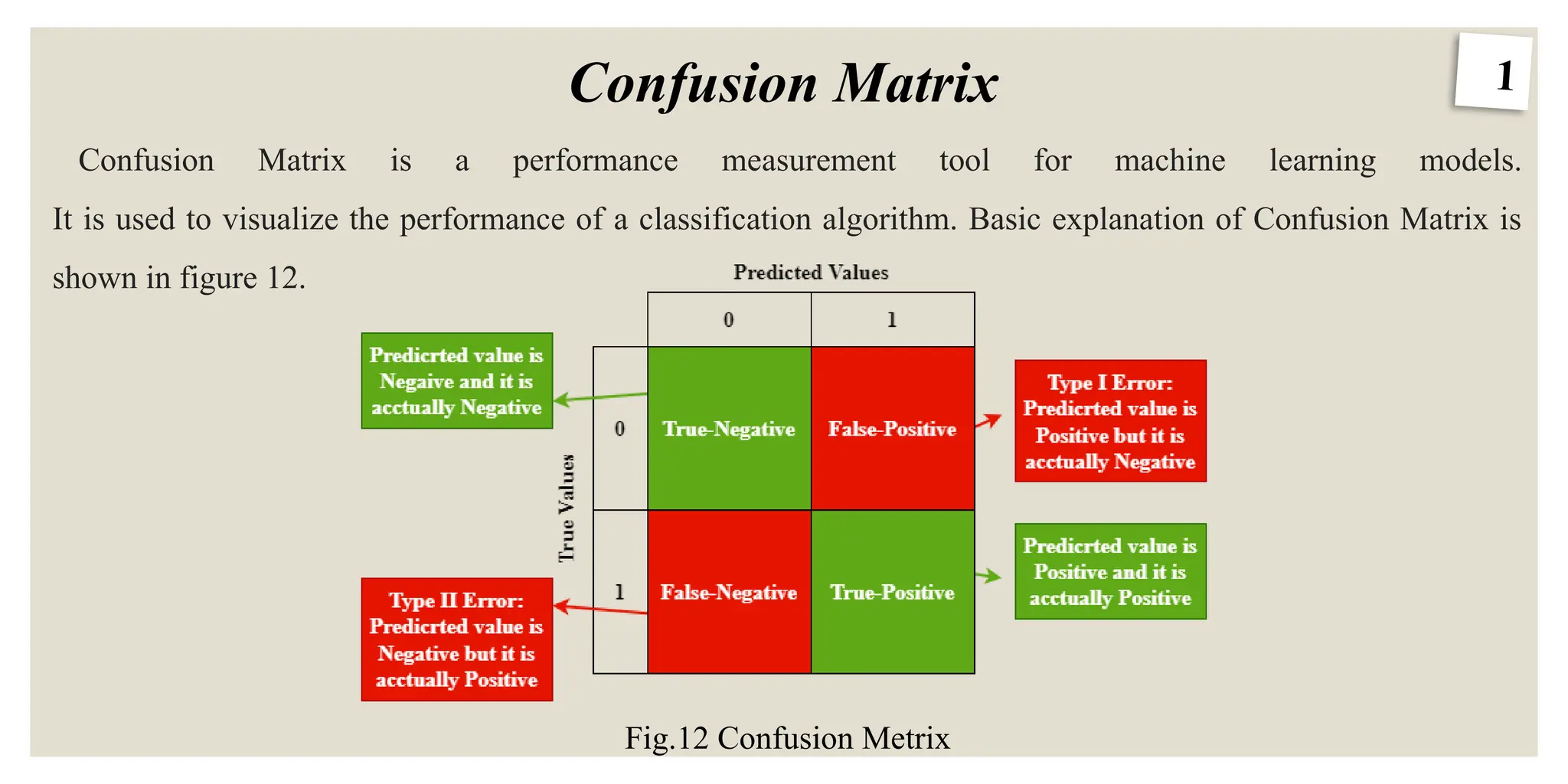
Confusion Matrix
Fig.12 Confusion Metrix
Confusion Matrix is a performance measurement tool for machine learning models.
It is used to visualize the performance of a classification algorithm. Basic explanation of Confusion Matrix is
shown in figure 12.

2. 2
Performance Parameters
All performance parameters, descriptions and their equations shown below.
Accuracy:
Accuracy represents the number of correctly classified data instances over the total number of data instances:
Precision:
A classification model's capability to determine only the most pertinent information points. Precision is
defined mathematically as shown below in equation 4.3.

3. 3
Performance Parameters
Recall:
An algorithm's capability to identify every applicable class within a data collection. We define recall statistically
as shown below:
F1 Score:
As illustrated below, the F1 score is determined as the harmonic average of the recall and precision scores. It
goes from 0 to 100%, with an elevated F1 score indicating a higher quality classifier.

4. 4
Machine Learning Algorithms
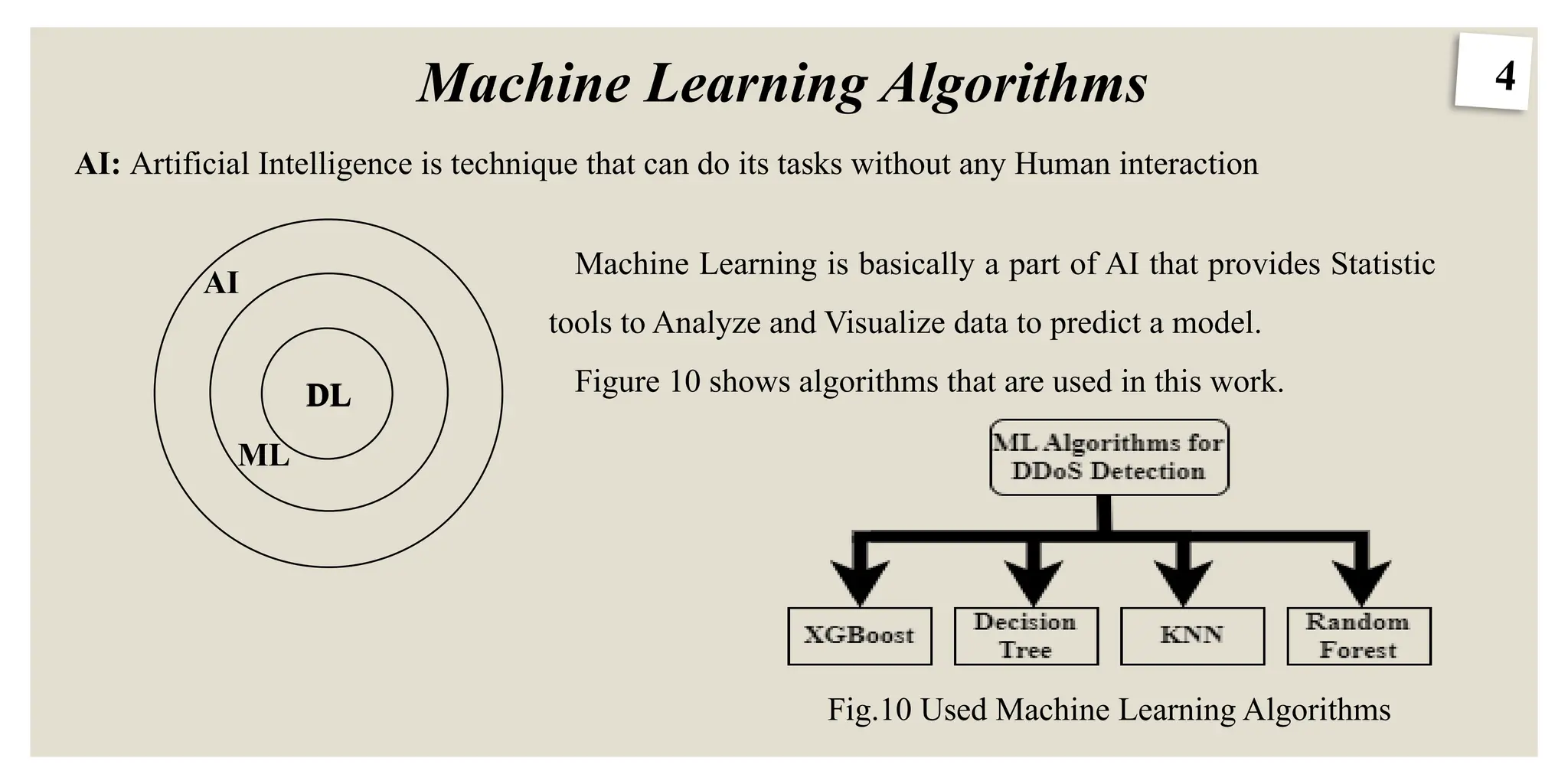
Fig.10 Used Machine Learning Algorithms
AI: Artificial Intelligence is technique that can do its tasks without any Human interaction
DL
ML
AI
DL
Machine Learning is basically a part of AI that provides Statistic
tools to Analyze and Visualize data to predict a model.
Figure 10 shows algorithms that are used in this work.

5. 5
KNN
The K-Nearest Neighbors (K-NN) algorithm is a popular Machine
Learning algorithm used mostly for solving classification problems.
Working of KNN:
The K-NN algorithm compares a new data entry to the values in a
given data set (with different classes or categories).
Based on its closeness or similarities in a given range (K) of neighbors,
the algorithm assigns the new data to a class or category in the data set
(training data).

6. 6
KNN
Step #1 - Load Data and Assign a value to K.
Step #2 - Calculate the distance between the new data entry and all other existing data entries (you'll learn
how to do this shortly). Arrange them in ascending order.
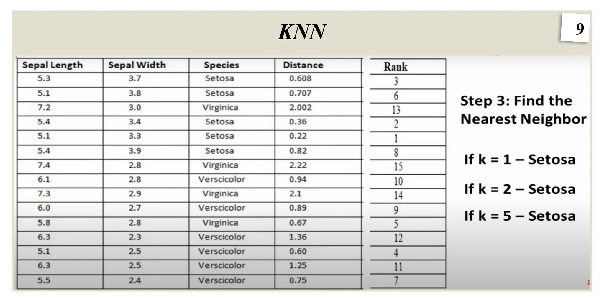
Step #3 - Find the K nearest neighbors to the new entry based on the calculated distances.
Step #4 - Assign the new data entry to the majority class in the nearest neighbors.
How do I choose K?
Selecting the optimal value of k depends on the characteristics of the input data. If the dataset has
significant outliers or noise a higher k can help smooth out the predictions and reduce the influence of
noisy data. However, choosing very high value can lead to underfitting where the model becomes too
simplistic.

7. 7
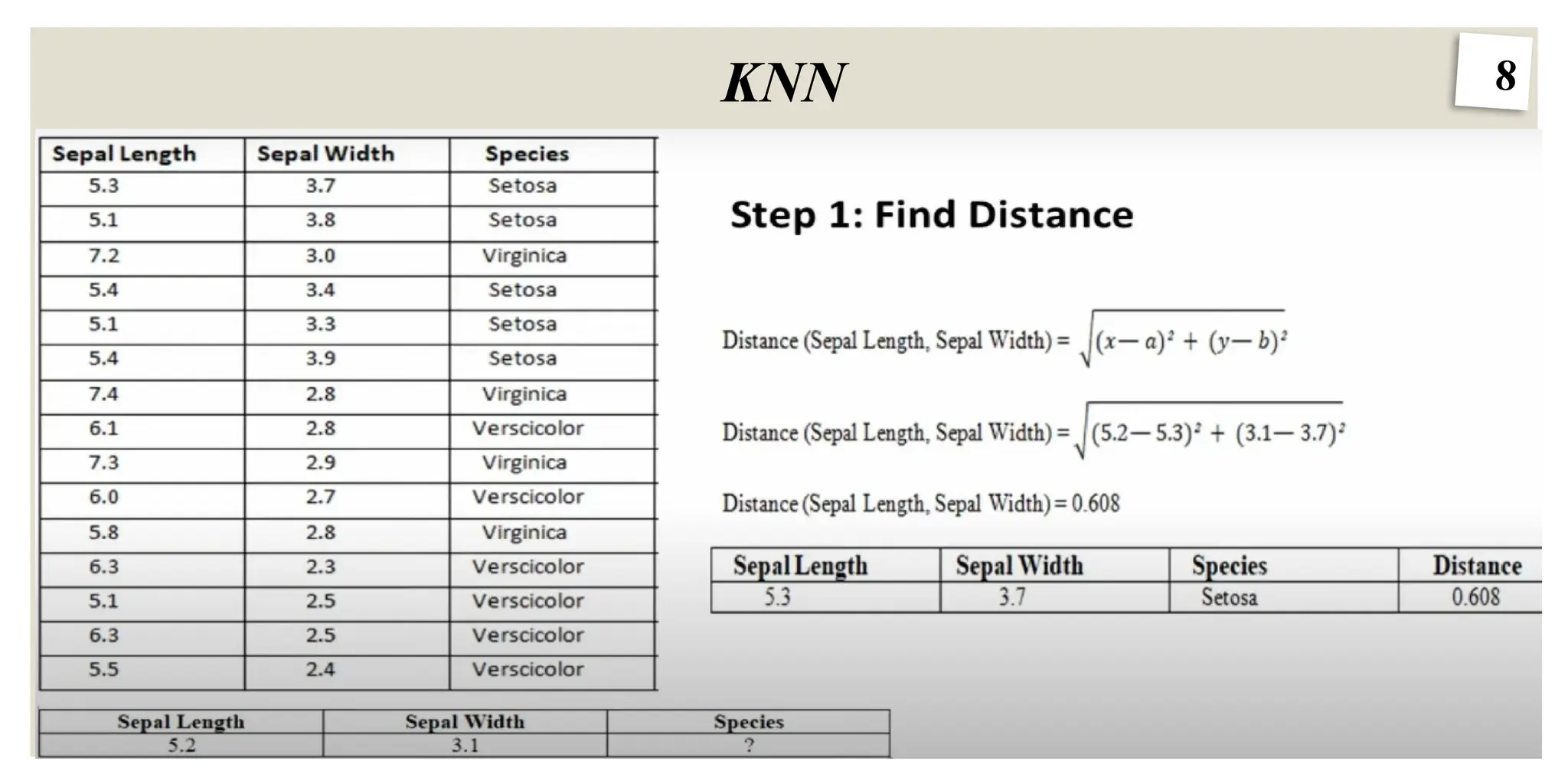
KNN
How does KNN work?
1. Euclidean Distance
We usually use Euclidean distance to calculate the nearest neighbor. If we have two points (x, y) and (a, b).
The formula for Euclidean distance (d) will be
d
2. Manhattan Distance
This is the total distance you would travel if you could only move along horizontal and vertical lines (like a
grid or city streets). It’s also called “taxicab distance” because a taxi can only drive along the grid-like streets
of a city.

8. 8
KNN

9. 9
KNN

10. 10
Decision Tree
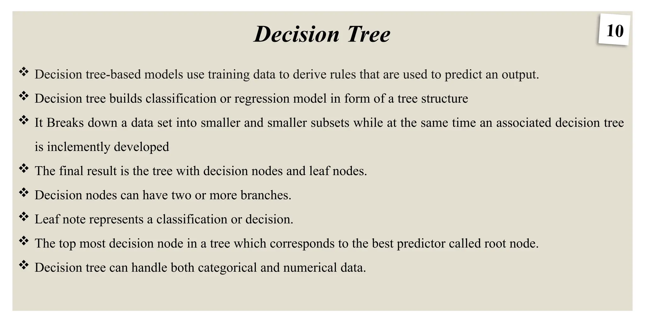
 Decision tree-based models use training data to derive rules that are used to predict an output.
 Decision tree builds classification or regression model in form of a tree structure
 It Breaks down a data set into smaller and smaller subsets while at the same time an associated decision tree
is inclemently developed
 The final result is the tree with decision nodes and leaf nodes.
 Decision nodes can have two or more branches.
 Leaf note represents a classification or decision.
 The top most decision node in a tree which corresponds to the best predictor called root node.
 Decision tree can handle both categorical and numerical data.

11. 11
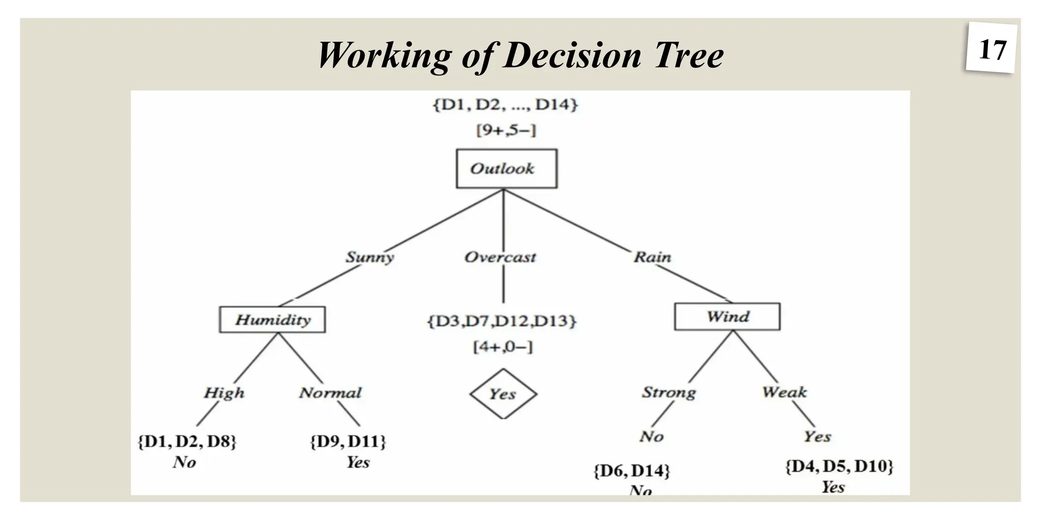
Working of Decision Tree
DT works on 2 basic parameters called (Entropy and Gini Index), Information Gain
 Entropy = -P+ log2 P+ - P- log2 P- (Entropy is a measurement of Randomness)
 Entropy Ranges from 0 to 1.
 Gini Index: The Gini Index, also known as Impurity, calculates the likelihood that somehow a randomly
picked instance would be erroneously cataloged.
 Gini Index = 1-[(P+)2
+ (P-)2
]
 GI ranges from 0 to 0.5
 P+ = Probability of True values
 P- = Probability of False values Fig. 11 Entropy vs Gini Impurity

12. 12
Working of Decision Tree
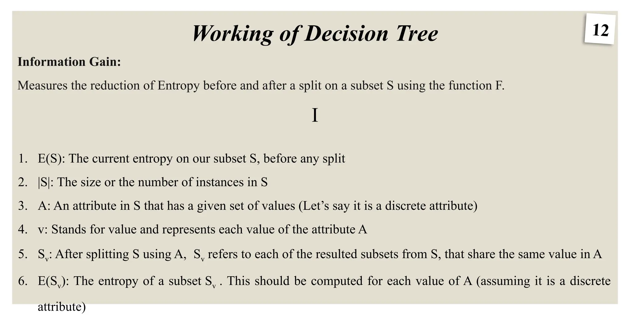
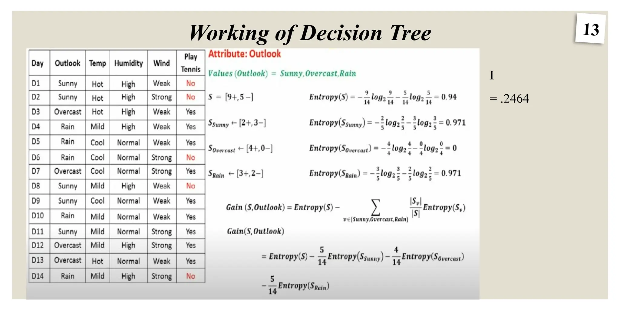
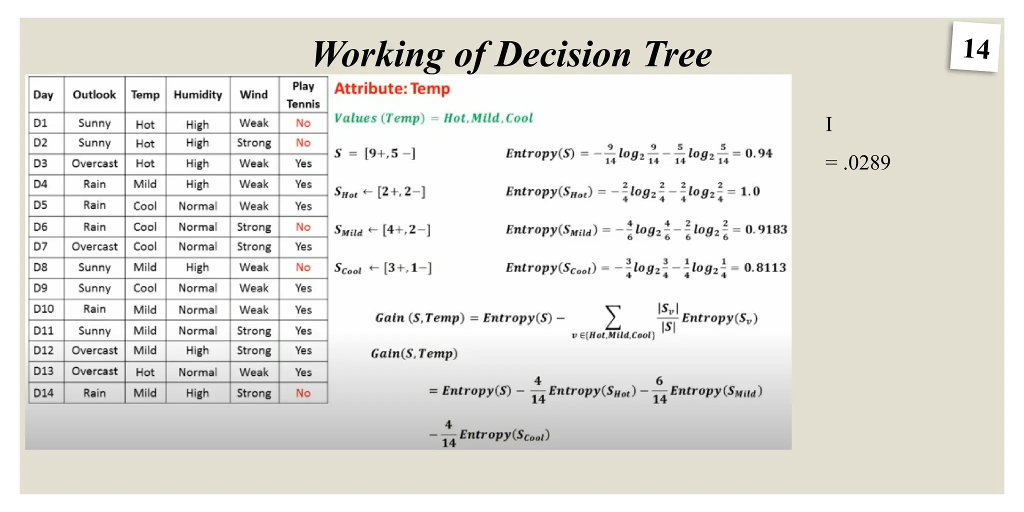
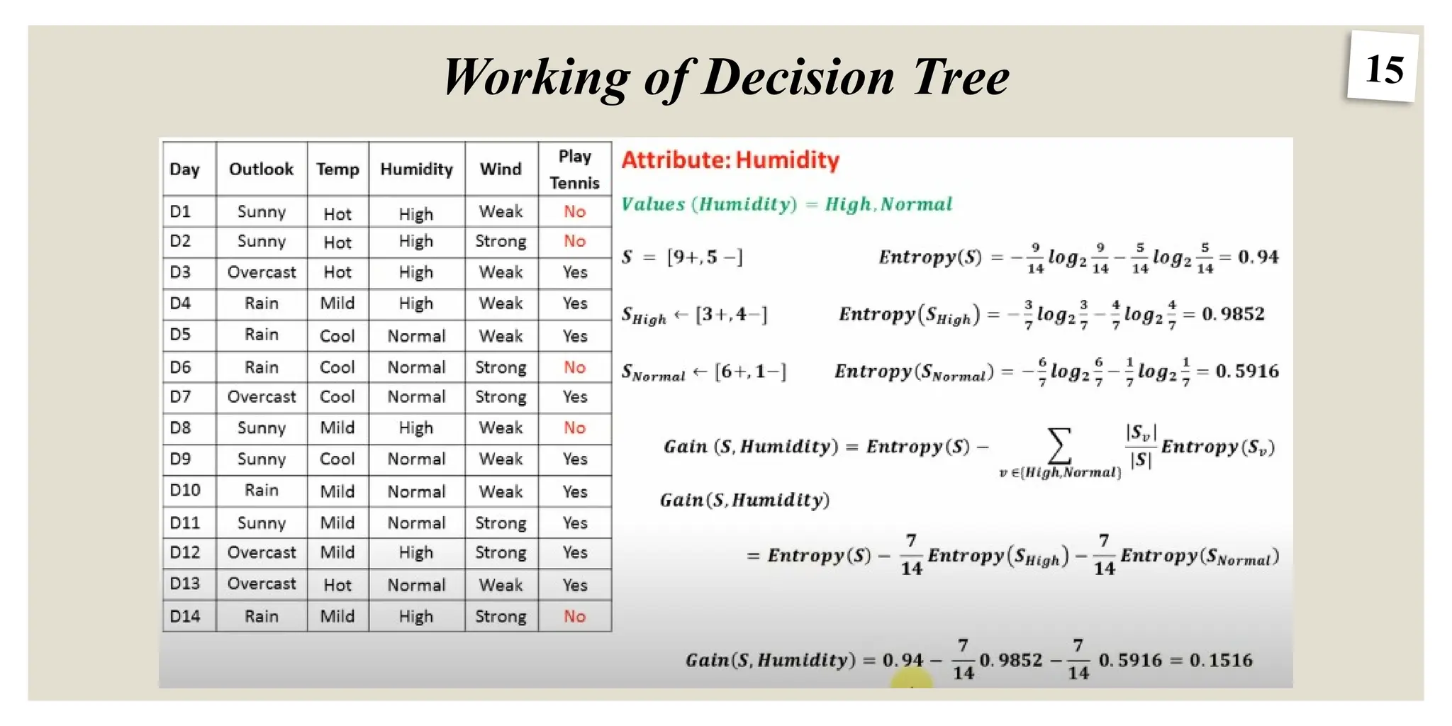
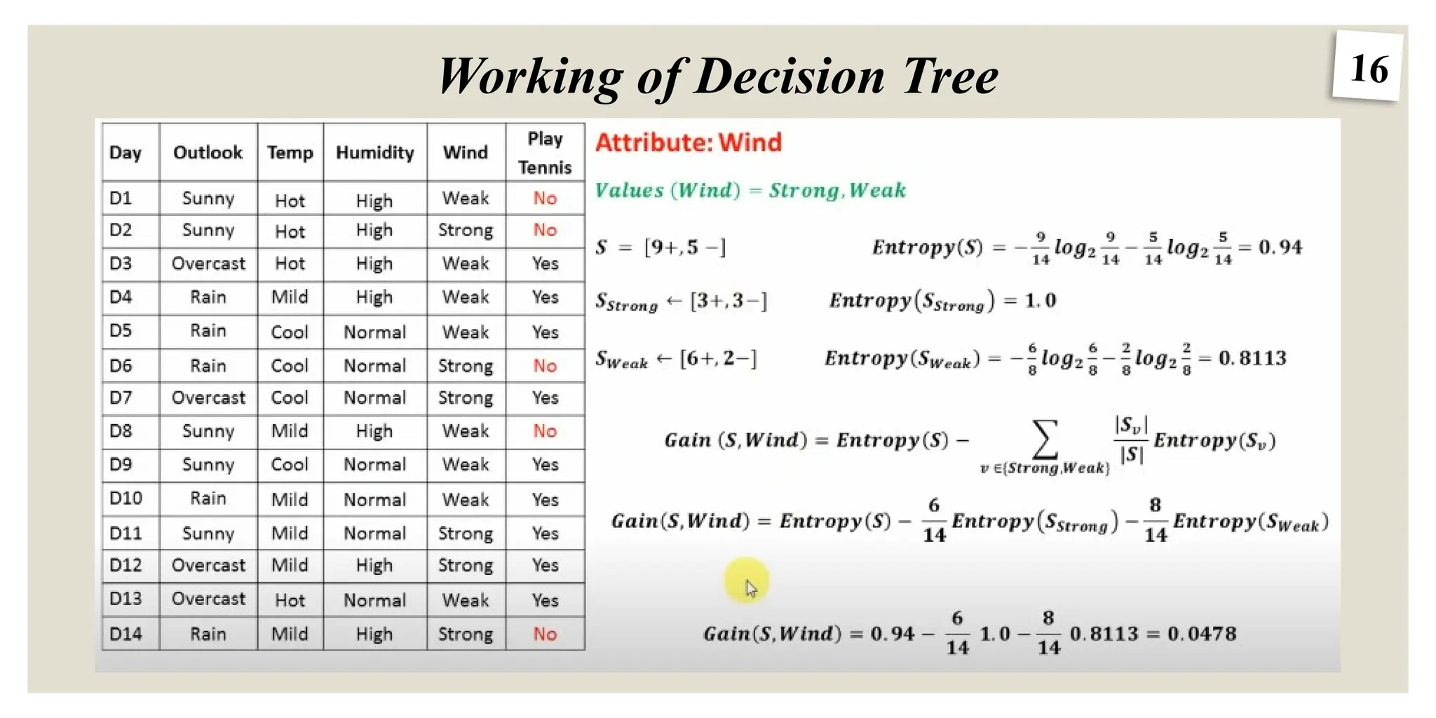
Information Gain:
Measures the reduction of Entropy before and after a split on a subset S using the function F.
I
1. E(S): The current entropy on our subset S, before any split
2. |S|: The size or the number of instances in S
3. A: An attribute in S that has a given set of values (Let’s say it is a discrete attribute)
4. v: Stands for value and represents each value of the attribute A
5. Sv: After splitting S using A, Sv refers to each of the resulted subsets from S, that share the same value in A
6. E(Sv): The entropy of a subset Sv . This should be computed for each value of A (assuming it is a discrete
attribute)

13. 13
Working of Decision Tree
vjh
I
= .2464

14. 14
Working of Decision Tree
I
= .0289

15. 15
Working of Decision Tree

16. 16
Working of Decision Tree

17. 17
Working of Decision Tree

18. 18
Decision Trees
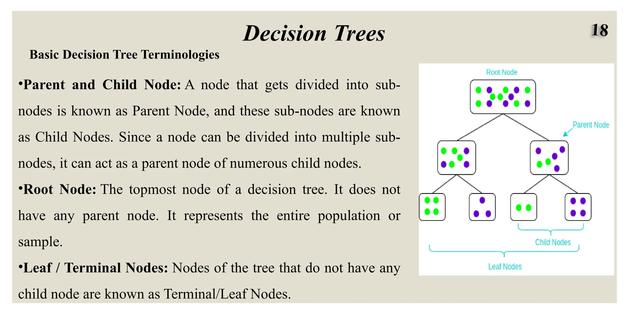
Basic Decision Tree Terminologies
•Parent and Child Node: A node that gets divided into sub-
nodes is known as Parent Node, and these sub-nodes are known
as Child Nodes. Since a node can be divided into multiple sub-
nodes, it can act as a parent node of numerous child nodes.
•Root Node: The topmost node of a decision tree. It does not
have any parent node. It represents the entire population or
sample.
•Leaf / Terminal Nodes: Nodes of the tree that do not have any
child node are known as Terminal/Leaf Nodes.

19. 19
Decision Trees
There are multiple tree models to choose from based on their
learning technique when building a decision tree, e.g., ID3,
CART, Classification and Regression Tree, C4.5, etc. Selecting
which decision tree to use is based on the problem statement. For
example, for classification problems, we mainly use a
classification tree with a gini index to identify class labels for
datasets with relatively more number of classes.

20. 20
Decision Trees
Node splitting, or simply splitting, divides a node into multiple sub-
nodes to create relatively pure nodes. This is done by finding the best
split for a node and can be done in multiple ways. The ways of splitting a
node can be broadly divided into two categories based on the type of
target variable:
1.Continuous Target Variable: Reduction in Variance
2.Categorical Target Variable: Gini Impurity, Information Gain, and
Chi-Square

21. 21
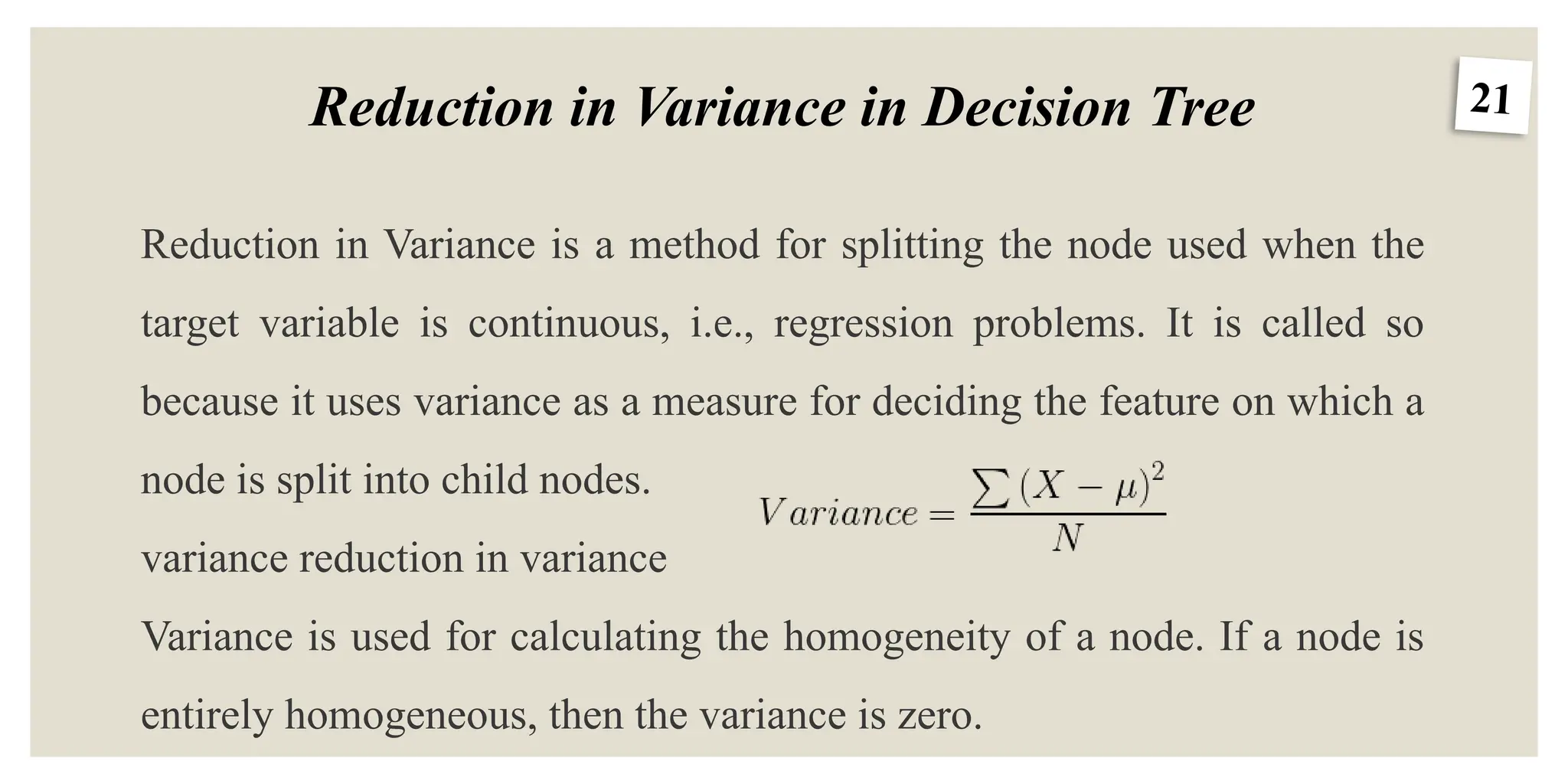
Reduction in Variance in Decision Tree
Reduction in Variance is a method for splitting the node used when the
target variable is continuous, i.e., regression problems. It is called so
because it uses variance as a measure for deciding the feature on which a
node is split into child nodes.
variance reduction in variance
Variance is used for calculating the homogeneity of a node. If a node is
entirely homogeneous, then the variance is zero.

22. 22
Reduction in Variance in Decision Tree
Here are the steps to split a decision tree using the reduction in variance
method:
1. For each split, individually calculate the variance of each child node
2. Calculate the variance of each split as the weighted average variance
of child nodes
3. Select the split with the lowest variance.
4. Perform steps 1-3 until completely homogeneous nodes are achieved

23. 23
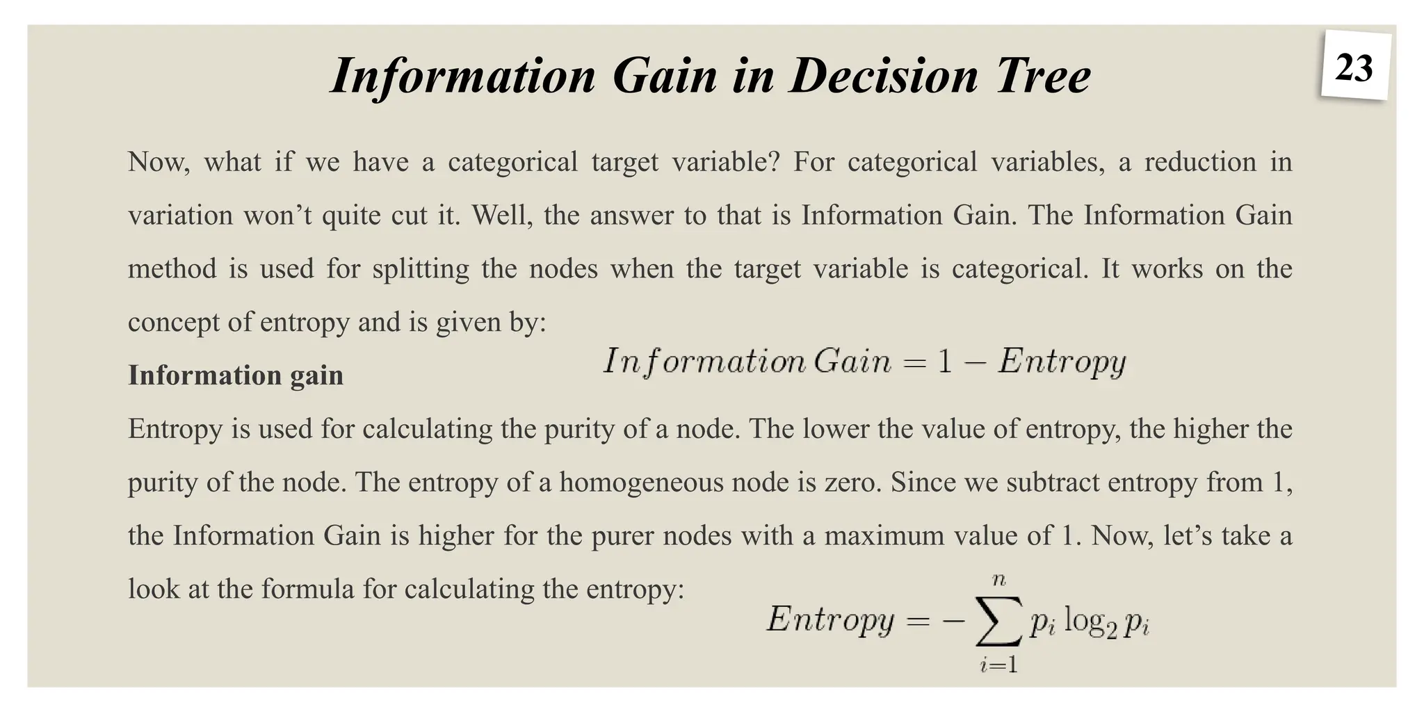
Information Gain in Decision Tree
Now, what if we have a categorical target variable? For categorical variables, a reduction in
variation won’t quite cut it. Well, the answer to that is Information Gain. The Information Gain
method is used for splitting the nodes when the target variable is categorical. It works on the
concept of entropy and is given by:
Information gain
Entropy is used for calculating the purity of a node. The lower the value of entropy, the higher the
purity of the node. The entropy of a homogeneous node is zero. Since we subtract entropy from 1,
the Information Gain is higher for the purer nodes with a maximum value of 1. Now, let’s take a
look at the formula for calculating the entropy:

24. 24
Information Gain in Decision Tree
Steps to split a decision tree using Information Gain:
1.For each split, individually calculate the entropy of each child node
2.Calculate the entropy of each split as the weighted average entropy of
child nodes
3.Select the split with the lowest entropy or highest information gain
4.Until you achieve homogeneous nodes, repeat steps 1-3

25. 25
Information Gain in Decision Tree
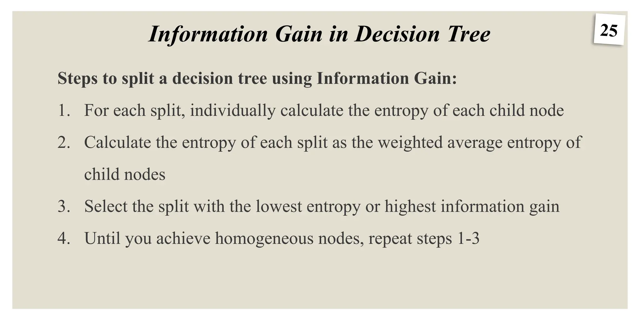
Steps to split a decision tree using Information Gain:
1. For each split, individually calculate the entropy of each child node
2. Calculate the entropy of each split as the weighted average entropy of
child nodes
3. Select the split with the lowest entropy or highest information gain
4. Until you achieve homogeneous nodes, repeat steps 1-3

26. 26
Gini Impurity in Decision Tree
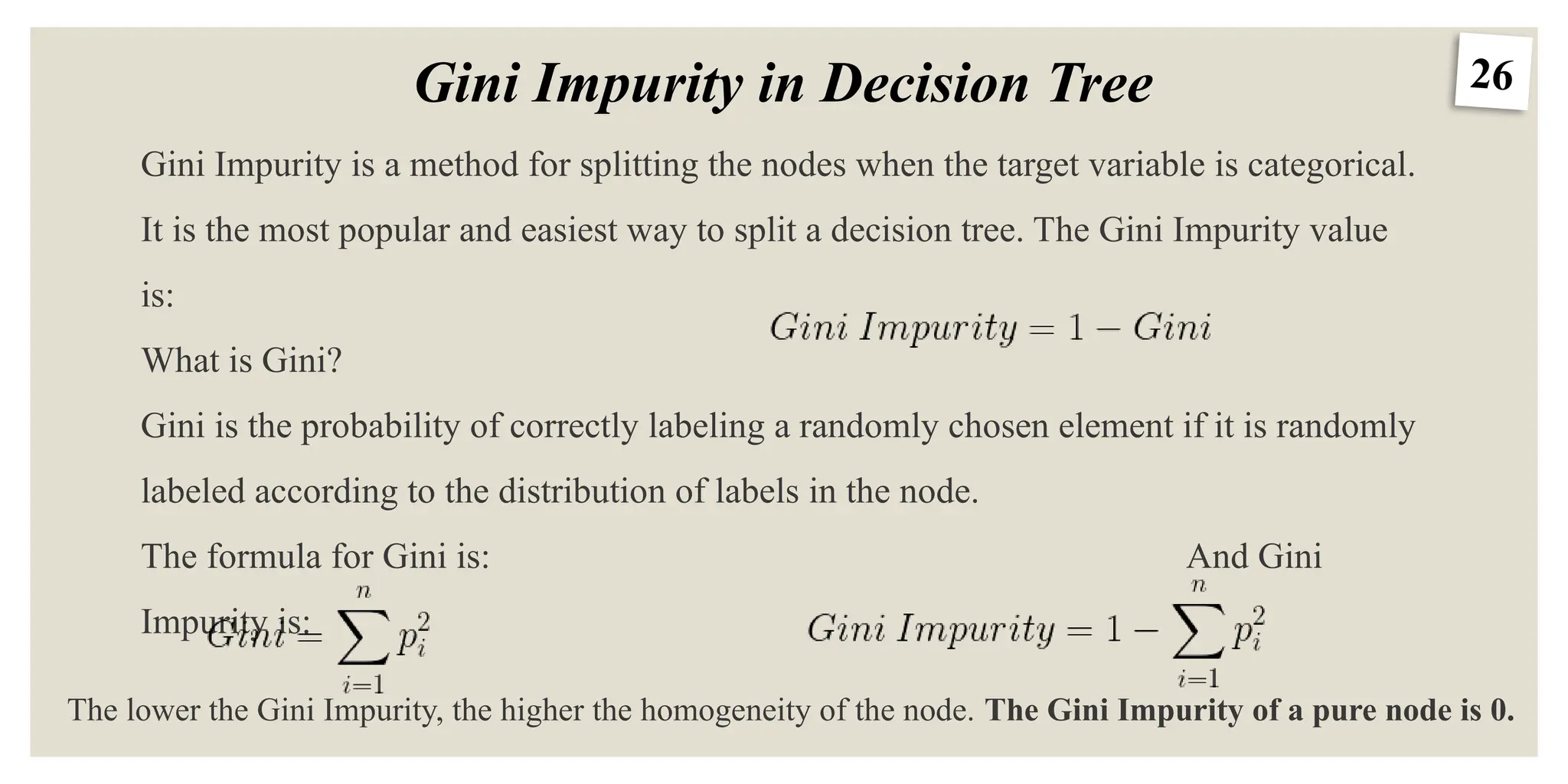
Gini Impurity is a method for splitting the nodes when the target variable is categorical.
It is the most popular and easiest way to split a decision tree. The Gini Impurity value
is:
What is Gini?
Gini is the probability of correctly labeling a randomly chosen element if it is randomly
labeled according to the distribution of labels in the node.
The formula for Gini is: And Gini
Impurity is:
The lower the Gini Impurity, the higher the homogeneity of the node. The Gini Impurity of a pure node is 0.

27. 27
Gini Impurity in Decision Tree
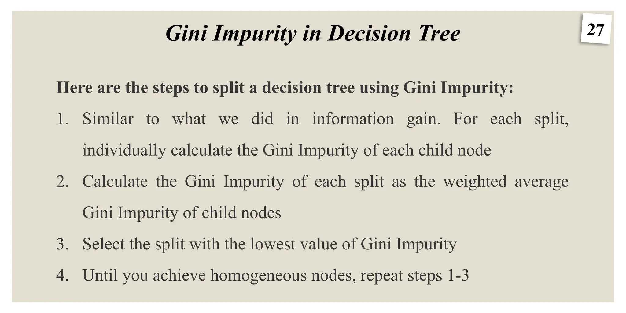
Here are the steps to split a decision tree using Gini Impurity:
1. Similar to what we did in information gain. For each split,
individually calculate the Gini Impurity of each child node
2. Calculate the Gini Impurity of each split as the weighted average
Gini Impurity of child nodes
3. Select the split with the lowest value of Gini Impurity
4. Until you achieve homogeneous nodes, repeat steps 1-3

28. 28
Chi-Square in Decision Tree
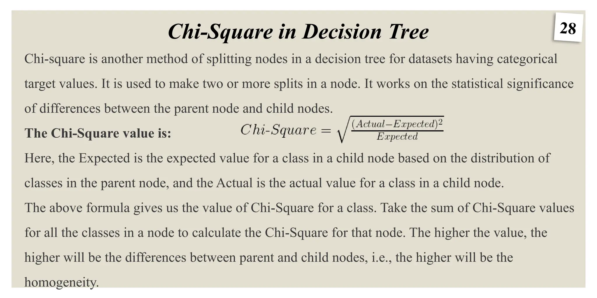
Chi-square is another method of splitting nodes in a decision tree for datasets having categorical
target values. It is used to make two or more splits in a node. It works on the statistical significance
of differences between the parent node and child nodes.
The Chi-Square value is:
Here, the Expected is the expected value for a class in a child node based on the distribution of
classes in the parent node, and the Actual is the actual value for a class in a child node.
The above formula gives us the value of Chi-Square for a class. Take the sum of Chi-Square values
for all the classes in a node to calculate the Chi-Square for that node. The higher the value, the
higher will be the differences between parent and child nodes, i.e., the higher will be the
homogeneity.

29. 29
Chi-Square in Decision Tree
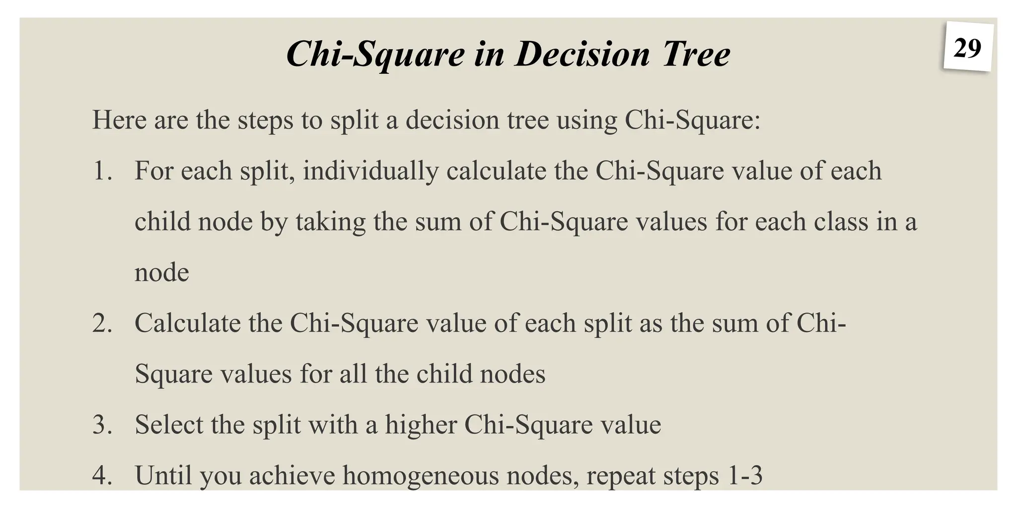
Here are the steps to split a decision tree using Chi-Square:
1. For each split, individually calculate the Chi-Square value of each
child node by taking the sum of Chi-Square values for each class in a
node
2. Calculate the Chi-Square value of each split as the sum of Chi-
Square values for all the child nodes
3. Select the split with a higher Chi-Square value
4. Until you achieve homogeneous nodes, repeat steps 1-3

30. 30
Ensemble Techniques
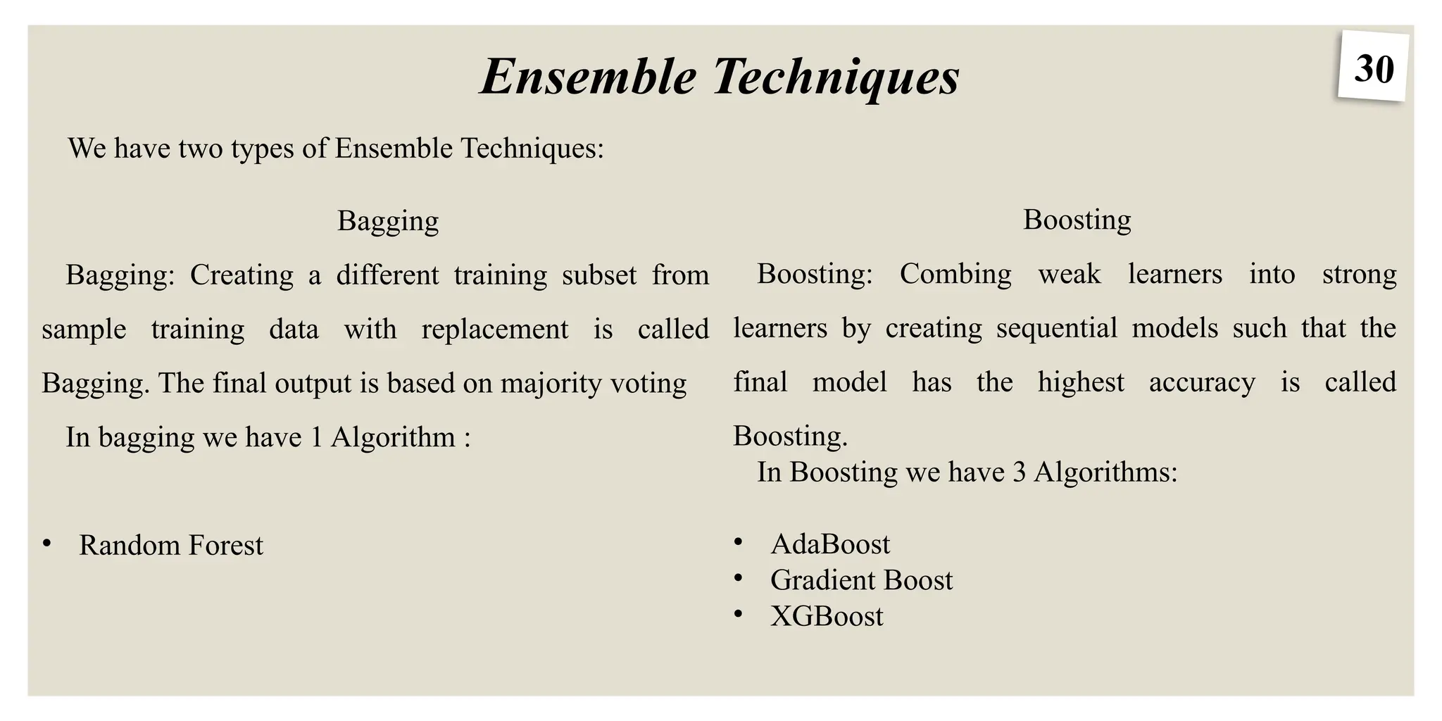
We have two types of Ensemble Techniques:
Bagging
Bagging: Creating a different training subset from
sample training data with replacement is called
Bagging. The final output is based on majority voting
In bagging we have 1 Algorithm :
• Random Forest
Boosting
Boosting: Combing weak learners into strong
learners by creating sequential models such that the
final model has the highest accuracy is called
Boosting.
In Boosting we have 3 Algorithms:
• AdaBoost
• Gradient Boost
• XGBoost

31. 31
Random Forest
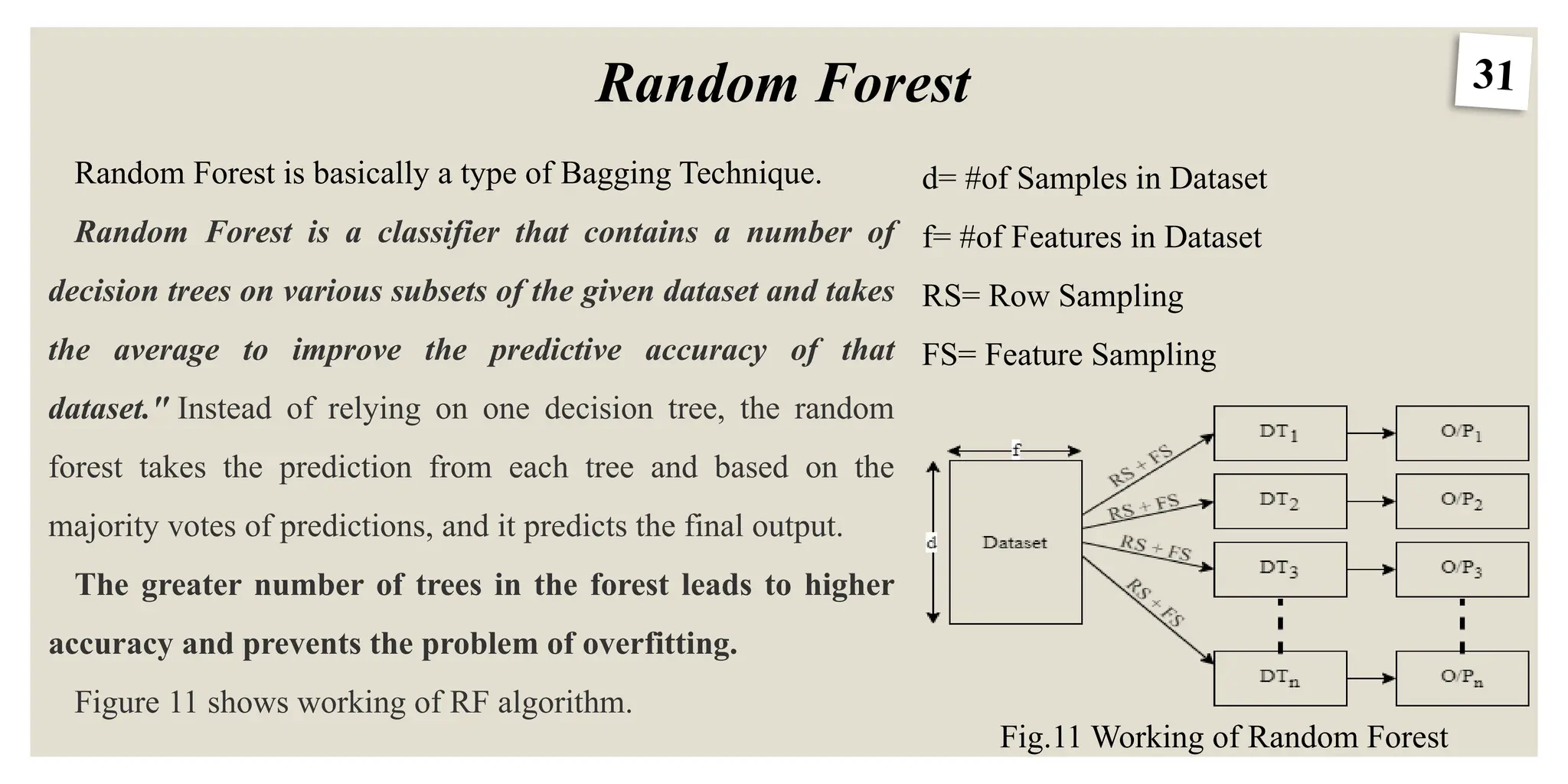
Fig.11 Working of Random Forest
Random Forest is basically a type of Bagging Technique.
Random Forest is a classifier that contains a number of
decision trees on various subsets of the given dataset and takes
the average to improve the predictive accuracy of that
dataset." Instead of relying on one decision tree, the random
forest takes the prediction from each tree and based on the
majority votes of predictions, and it predicts the final output.
The greater number of trees in the forest leads to higher
accuracy and prevents the problem of overfitting.
Figure 11 shows working of RF algorithm.
d= #of Samples in Dataset
f= #of Features in Dataset
RS= Row Sampling
FS= Feature Sampling