The document discusses various database indexing and joining techniques. It provides details on different types of indexes like B+ tree, bitmap indexes and hash indexes. It also explains different join algorithms like nested loops joins, merge joins and hash joins. It describes how these indexes and joins are used by the query optimizer to generate and select the most efficient execution plan for a given SQL query.

1. © 2008 Hewlett-Packard Development Company, L.P.
The information contained herein is subject to change without notice
DB

2. Agenda
• Cost Model
• Index(Scans)
• Statistics/Histograms
• SQL general process/Optimizer
• Joins
• Data Skew (HASH)
• DB/Server architecture : general/Shared
everything/Shared nothing vs SMP/NUMA/MPP
• Neoview Architecture (MPP)

3. © 2008 Hewlett-Packard Development Company, L.P.
The information contained herein is subject to change without notice
New vision

4. Agenda
• Technical trend/ BI trend
• Vertica: basic/projection/ encoding&compression
• In-Memory DB: general theory
• SSD
• Hadoop: ecosystem/HDFS/MapReuce/Future
• Sqoop/Pig/Hive/Hbase
• Autonomy

5. © 2008 Hewlett-Packard Development Company, L.P.
The information contained herein is subject to change without notice
Overview

6. Overview

7. CAP
Availability
Consistency
Tolerance to
network
Partitions
CP:
BigTable, Hbase,
MongoDB, Berkeley
DB…
CA:
RDBMs, like Oracle,
MySQL
Vertica
TimesTen
AP:
Dynamo,
KAI,
Tokyo Cabinet
Riak

8. © 2008 Hewlett-Packard Development Company, L.P.
The information contained herein is subject to change without notice
Cost Model

9. Cost Model
• The cost model is based on a description of the
database schema and size, and looks at statistics for
the attribute values in each table involved in queries.
• The cost model will typically includes estimates for
resource consumption for different plan possibilities
such as CPU, memory, network bandwidth, and
input/output(I/O).
• The cost model will also determine, based on the
physical design of the database, whether an index
should be exploited, such as which indexes to access
or what join method to use (Nest-loop join, Sorted
Merge join, Hash Join).

10. Cost Model
• Much of the literature on automated physical design
has focused on the possibility of “what-if analysis” using
the database’s existing query optimizer.
• “What-if analysis” is the art of carefully lying to the
query optimizer and observing the impact.

11. Cost Model
• I/O Time Cost – Individual Block Access
• Block access cost = disk access time to a block from a random starting
location = average disk seek time + average rotational delay + block
transfer
• I/O Time Cost – Table Scan and Sorts
• Network Time Delays
• Network delay = propagation time + transmission time
Where Propagation time = network distance/propagation speed
And Transmission time = packet size/network transmission rate
• CPU Time Delays
• Example: Operator Cost =
Cf1(CPU_COST)+W2*Cf2(Network_Cost)+W3*Cf3(Ra
ndom_Ios)+W4*Cf4(Sequential_Ios)

12. © 2008 Hewlett-Packard Development Company, L.P.
The information contained herein is subject to change without notice
Index

13. Index
• An Index is a data organization set up to speed up the
retrieval (query) of data from tables.
• Types:
• Unique index (B+ Tree/ On key)
• Secondary Index/Nonunique index (B+ Tree/Bitmap Index)
• Clustered Index/Nonclustered Index (B+ Tree)
• Hash Index (B+ Tree/ On Key)

14. Index – Basic Indexing Methods
• B+ Tree

15. Index – Basic Indexing Methods
• Bitmap Index
Male 0 0 0 1 0 0 0 0 0
Fem
ale
1 1 1 0 1 1 1 1 1

16. 16
Unique access
• Primary key is supplied
• Includes hash key
• Exact target partition
• Determined by hash key
• B-tree is used to locate data
block
• Row is retrieved and returned
Week Store Item
1/7/90 1 1
1/14/90
1 3
1
2
3
3
4
4
. . .
. . .
1/7/90
1/7/90
1/7/90
1/7/90
1/7/90
1/7/90
1/7/90
1/14/90
1/14/90
1/14/90
1/14/90
1/14/90
1/14/90
1/14/90
1
1
1
1
3
3
4
4
5
34
13
3
2
4
2
4
5
35
1
20
11
12
. . .
. . .
. . .
. . .
. . .
. . .
. . .
. . .
. . .
. . .
. . .
. . .
. . .
. . .
. . .
Where:
week = ‘1/7/90’,Store = 4, Item = 4

17. 17
Subset scan
• Partial key is supplied
• Leading prefix of columns
• May/may not include hash key
• Exact target partition
• If full hash key supplied
• Otherwise all partitions accessed
• B-tree is used to locate first data block
• Begin-key and/or end-key for positioning
• Rows retrieved until ending condition is met
Week Store Item
1/7/90 1 1
1/14/90
1 3
1
2
3
3
4
4
. . .
. . .
1/7/90
1/7/90
1/7/90
1/7/90
1/7/90
1/7/90
1/7/90
1/14/90
1/14/90
1/14/90
1/14/90
1/14/90
1/14/90
1/14/90
1
1
1
1
3
3
4
4
5
34
13
3
2
4
2
4
5
35
1
20
11
12
. . .
. . .
. . .
. . .
. . .
. . .
. . .
. . .
. . .
. . .
. . .
. . .
. . .
. . .
. . .
Where:
week = ‘1/7/90’
Store between 3 and 4

18. 18
Full scan
• No partial key access
• No hash key
• may filter rows based on
predicates
– Where <data_col> = ….
• may aggregate results
– SUM (data_col) …
Week Store Item
1/7/90 1 1
1/14/90
1 3
1
2
3
3
4
4
. . .
. . .
1/7/90
1/7/90
1/7/90
1/7/90
1/7/90
1/7/90
1/7/90
1/14/90
1/14/90
1/14/90
1/14/90
1/14/90
1/14/90
1/14/90
1
1
1
1
3
3
4
4
5
34
13
3
2
4
2
4
5
35
1
20
11
12
. . .
. . .
. . .
. . .
. . .
. . .
. . .
. . .
. . .
. . .
. . .
. . .
. . .
. . .
. . .

19. Why a Full table scan id faster for accessing
large amounts of Data?
• Full table scans are cheaper than index range scans
when accessing a large fraction of blocks in a table.
• Full table scans can use larger I/O calls, and making
fewer large I/O calls is cheaper than making many
smaller calls.

20. © 2008 Hewlett-Packard Development Company, L.P.
The information contained herein is subject to change without notice
Statistics/Histogram
s

21. Statistics
• The resulting statistics provide the query optimizer with
information about data uniqueness and distribution,
Using this information, the query optimizer is able to
compute plan costs with a high degree of accuracy and
choose the best execution plan on the least cost.
• Include:
• Table statistics: Number of rows/Number of blocks/Average row
length
• Column Statistics: Number of distinct values in column/ Number of
nulls in column/ Data distribution (Histogram)/ Extended Statistics
• Index Statistics: Number of leaf blocks/ levels/ clustering factor
• System statistics: I/O performance and utilization/ CPU performance
and utilization

22. What it used for?
• The basic information for choosing a query plan based
on the cost model:
• System statistics will give the value for CPU, I/O with
Disk and network.
• Index will give the value do we have the index, if have,
what’s the cost.
• Table will give the basic value the block access cost for
this table and record.
• The most important: Column Statistics will demonstrate
the best way to access the data.
• But not that simple, let’s dig more deep in SQL
process.

23. Data distribution (Histogram)
• It is import to calculate the correct cardinality at each
stage of an execution plan, because the cardinality at
any one point in the plan can affect join orders, join
methods, and choice of indexes.
• Many DB use Histograms to improve its selectivity and
cardinality calculations for nununiform data
distributions: two types: Frequency histogram (less
buckets)/ Height balanced histogram(more buckets).

24. Why?
• For example:
• If we don’t collect histogram, if a table have values from
1 to 9, total 900 records, the DB will assume that every
value have 100 records.
• But actually, the value 1 have 800 records, so if we
choose 1, the full table scan will have better
performance, but for others, using index will gain better
performance.
• So the DB will chose the wrong execution plan for this
query.

25. © 2008 Hewlett-Packard Development Company, L.P.
The information contained herein is subject to change without notice
SQL general
process/Optimizer

26. General process

27. More Details
Optimization
Parsing
SQL
Statements
Syntax Check
Semantic
Check
Shared Pool
Check
Logic Query
Plan
Query
Transformer
Estimator
Physical Plan
Generator
Data Dictionary
Execution
Soft Parse
Hard Parse
Statistics

28. Parsing
• After Syntax Check/Semantic Check, to generate all
possible logical query plans, a tree structure.
• Syntax Check: Key word, Relational, Attribute,
Symbols/grammar; So if your statement contains a
syntax error, here returns the error message to the
client and stop.
• Semantic Check/Pre-Processor: Relation must be exist
in the current schema/Attribute exists?/Type
• More complex, the access and access right, type error,
attribute missing, alias error like the two table have the
same alias and so on, will happen here.

29. Optimizer Operations
• When the user submits a SQL statement for execution,
the optimizer performs the following steps:
• 1. The optimizer generate a set of potential plans for
the SQL statements based on available access paths
and hints
• 2. The optimizer estimates the cost of each plan based
on statistics in the data dictionary. Statistics include
information on the data distribution and storage
characteristics of the tables, indexes, and partitions
accessed by the statement. The cost is an estimated
value proportional to the expected resource use
needed to execute the statement with a particular plan.
The optimizer calculates the cost of access paths and
join

30. Optimizer Operations -- continued
• orders based on the estimated computer resources,
which includes I/O, CPU, and memory.
• Serial plans with higher costs take longer to execute
than those with smaller costs. When using a parallel
plan, resource use is not directly related to elapsed
time.
• 3. The optimizer compares the plans and chooses the
plan with lowest cost.
• The output from the optimizer is an execution plan that
describes the optimum method of execution. The plan
shows the combination of the steps Oracle Database
uses to execute a SQL statement. Each step either
retrieves rows physically from the database or prepares
them for the user issuing the statement.

31. Optimizer Operations -- continued
Operation Description
Evaluation of expressions and
conditions
The optimizer first evaluates
expressions and conditions containing
constants as fully as possible
Statement Transformation For complex statements involving, for
example, correlated subqueries and
views, the optimizer might transform the
original statement into an equivalent join
statement
Choice of optimizer goals The optimizer determines the goal of the
optimization
Choice of access paths For each table accessed by the
statement ,the optimizer chooses one or
more of the available access to obtain
the table data
Choice of Join orders For a join statement that joins more than
two tables, the optimizer choose which
pair of table is joined first, and which
table is joined to the result.

32. Example: Logical Query Plans
• All possible plans
• SELECT P.Pname from P, SH, S WHERE P.Pnum =
SH.Pnum AND SH.Snum = S.Snum AND S.city = ‘NY’;
3 Tables, 3! Possible plans:
1. S join SH join P
2. SH join S join P
3. P join SH join S
4. SH join P join S
5. S*P join SH (P and S have no join condition)
6. P*S join SH (P and S have no join condition)

33. Logical to Physical Query Plan
• CBO
• 1. get all logical plans
• 2. filter the worst based on algorithm like Cartesians
• 3. Computer the cost and get the lowest, then transfer
the chosen one to Physical Query Plan include how
data are accessed(table scan), joined, computed…

34. © 2008 Hewlett-Packard Development Company, L.P.
The information contained herein is subject to change without notice
Joins

35. Nested joins
• Operation and characteristics
• A row from the outer table is used to probe the inner table
for a match of one or more rows
– A buffer of rows is normally read from the outer table, and
each row in turn is used to probe the inner table
• One message is sent to the inner table for each outer row
• Tends to be selected when relatively few probes into the
inner table are expected, when the inner table is large
• Access rules regarding hash keys apply

36. Nested Join - Algorithms
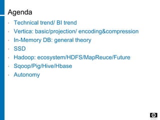
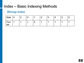
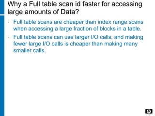
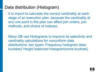
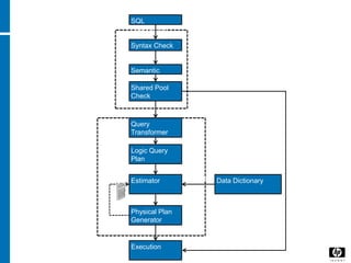
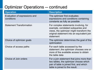
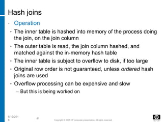
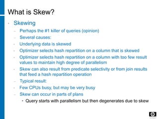
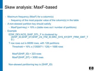
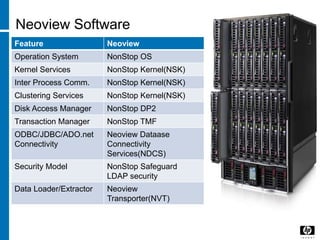
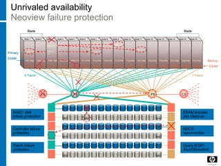
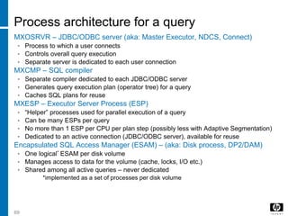
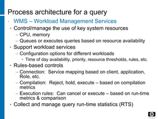
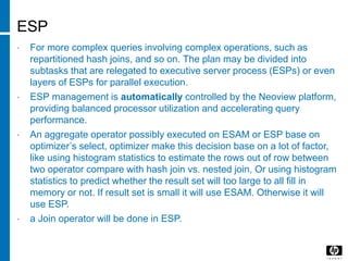
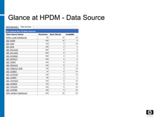
• SELECT * FROM TABLE1, TABLE 2 WHERE
TABLE1.COL1= TABLE2.COL1
36 [Rev. # or date] – HP Restricted
COL1 COL2
1 1
2 2
3 0
4 4
6 6
7 7
COL1 COL2
1 1
3 0
3 1
4 4
5 5
6 6
Join Results
1,1,1,1
3,0,3,0
3,0,3,1
4,4,4,4
6,6,6,6
Table2Table1

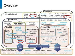
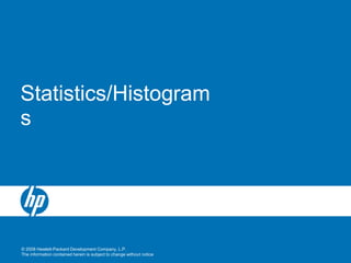
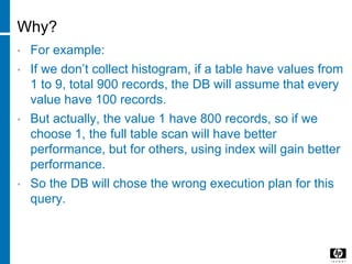
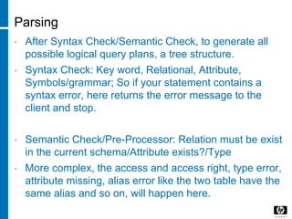
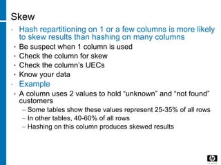
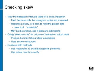
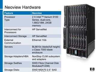
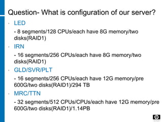
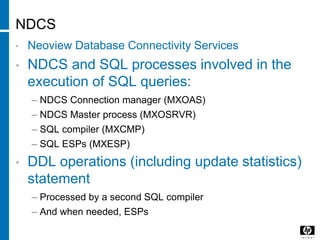
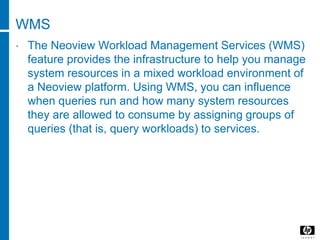
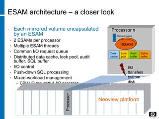
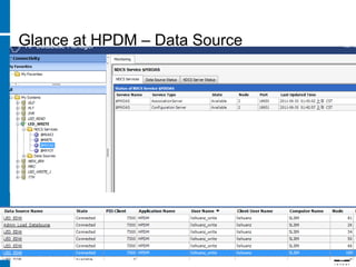
37. Nested Join - Algorithms
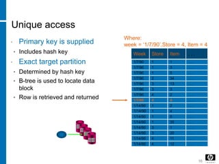
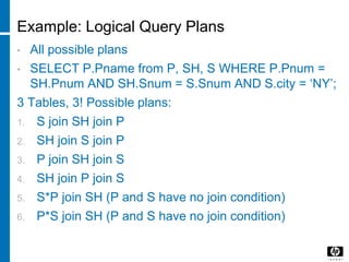
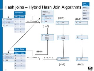
1,1
2,2
3,0
4,4
6,6
7,7
37 [Rev. # or date] – HP Restricted
1,1 3,0 3,1 4,4 5,5 6,6
Table2 (INNER)
Table1(Outer)

38. Nested join efficiency
• When the NJ includes the hash key for the inner table
only one target partition is accessed for each outer row
• When the NJ does not include the hash key for the
inner table every target partition is accessed for each
outer row
• Work Best:
• If the inner scan is a keyed access
• The number of outer probes/rows is small
• This can be very costly

39. Merge joins
• Operation
• Both tables are required to be sorted on the join column
• A buffer of rows is read from the inner and outer tables
• A row from the outer table is used to match inner table rows,
in a “match-merge” pattern (simplified description)

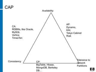
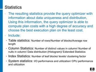
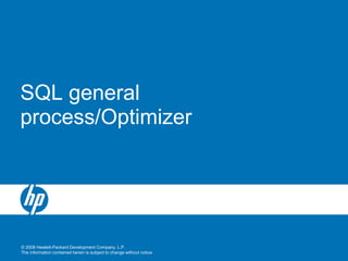
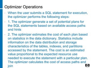
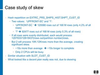
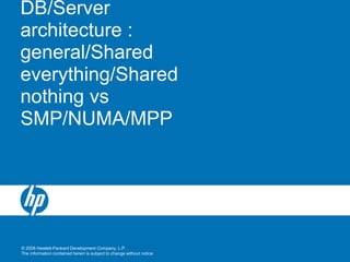
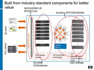
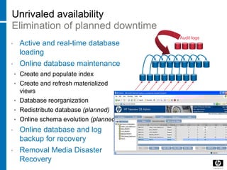
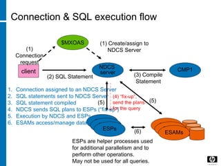
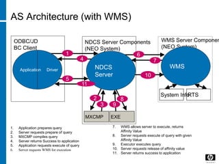
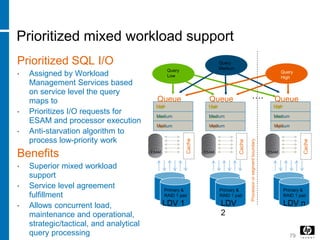
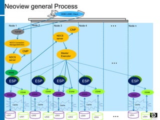
40. Merge Join - Algorithms
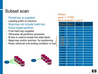
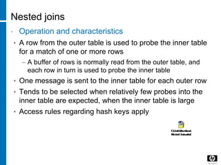
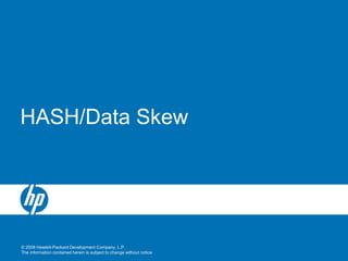
1,1
2,2
3,0
4,4
6,6
7,7
40 [Rev. # or date] – HP Restricted
1,1 3,0 3,1 4,4 5,5 6,6
Table2 (INNER)
Table1(Outer)
Means
Search Space

41. 6/12/201
6 Copyright © 2005 HP corporate presentation. All rights reserved.
41
Hash joins
• Operation
• The inner table is hashed into memory of the process doing
the join, on the join column
• The outer table is read, the join column hashed, and
matched against the in-memory hash table
• The inner table is subject to overflow to disk, if too large
• Original row order is not guaranteed, unless ordered hash
joins are used
• Overflow processing can be expensive and slow
– But this is being worked on

42. Hash joins – Hybrid Hash Join Algorithms
0 3,0 3,1 6,6
1 1,1 4,4
2 5,5
42
COL1 COL2
1 1
3 0
3 1
4 4
5 5
6 6
Inner Table
0 3,0 6,6
1 1,1 4,4 7,7
2 2,2
COL1 COL2
1 1
2 2
3 0
4 4
6 6
7 7
Outer Table
H = COL1 mod 3
H = COL1 mod 3
Memory-
resident hash
table
0 3,0 6,6
(H=0)
0 3,0,3,0
3,0,3,1
6,6,6,6
(H=0)
H = 1, H = 2
1 1,1 4,4 7,7 2 2,2
1 1,1 4,4 2 5,5
1 1,1 4,4 7,7
2 2,2
1 1,1,1,1
4,4,4,4
2
Join
Results
1,1,1,1
3,0,3,0
3,0,3,1
4,4,4,4
6,6,6,6
(H=1)
(H=1)
(H=2)
(H=2)

43. © 2008 Hewlett-Packard Development Company, L.P.
The information contained herein is subject to change without notice
HASH/Data Skew

44. Partition (HASH)
• Simply divide big table or index into small parts, which
could be more manageable .
• Types:
• Range Partition
• List Partition
• Hash partition (Prefered)

45. What is Skew?
• Skewing
– Perhaps the #1 killer of queries (opinion)
– Several causes:
• Underlying data is skewed
• Optimizer selects hash repartition on a column that is skewed
• Optimizer selects hash repartition on a column with too few result
values to maintain high degree of parallelism
• Skew can also result from predicate selectivity or from join results
that feed a hash repartition operation
– Typical result:
• Few CPUs busy, but may be very busy
– Skew can occur in parts of plans
• Query starts with parallelism but then degenerates due to skew

46. Skew
• Hash repartitioning on 1 or a few columns is more likely
to skew results than hashing on many columns
• Be suspect when 1 column is used
• Check the column for skew
• Check the column’s UECs
• Know your data
• Example
• A column uses 2 values to hold “unknown” and “not found”
customers
– Some tables show these values represent 25-35% of all rows
– In other tables, 40-60% of all rows
– Hashing on this column produces skewed results

47. Case study of skew
• Hash repartition on EXTRC_PRS_SHIPS_HIST.SHPT_CUST_ID
− Two values: ‘UPFRONT-SC’ and ‘?’:
• ‘UPFRONT-SC ’  120088 rows out of 168 M rows (only 4.2% of all
rows)
• ‘?’  92477 rows out of 168 M rows (only 5.3% of all rows)
− If all rows were evenly distributed, each would process
1207933/128=9437(rows out/partition number)rows.
− But 2 will process 10K-12Krows more than the average, creating
significant skew.
• ~10x more than average  ~10x longer to complete
• Only 2 CPUs will be busy
• Similar situation with SLDT_CUST_ID
• What looked like a decent plan really was not, due to skewing

48. Skew analysis: UEC-based
• A non-skewed partition key should satisfy
− UEC(part-key) > 50 x number of partitions in table
• Example
EDW_DEV.ACQ_SHIP_DTL_F is clustered by
(SHIP_ID,SHIP_DT,SHIP_LN_ITM_ID,SRC_SYS_KY,EFF_FRM_GMT_T
S ) with 128 partitions
Threshold = 50 x 128 = 5,120 UECs
UEC(SHIP_ID) = 91303 UEC(SHIP_DT) = 1292
UEC(SHIP_LN_ITM_ID) = 247 UEC(SRC_SYS_KY) = 1
UEC(EFF_FRM_GMT_TS) = 18,244
Candidates for non-skewed partitioning key are:
(SHIP_ID)
(SHIP_DT)

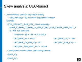
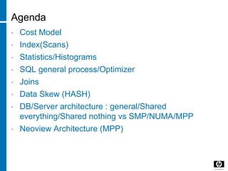
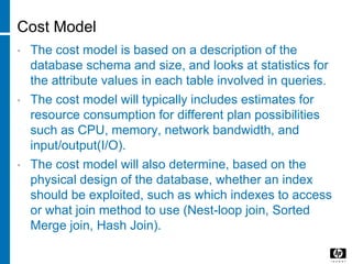
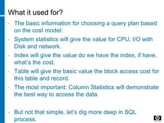
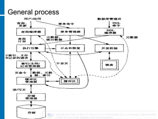
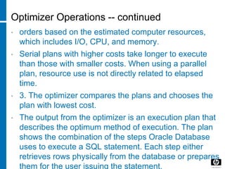
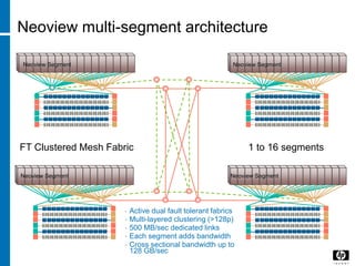
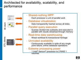
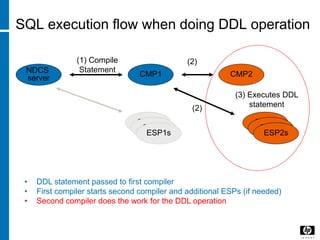
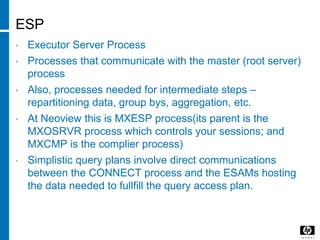
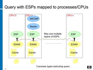
49. Skew analysis :Command to check UECs
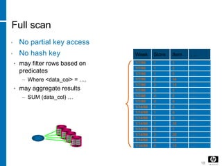
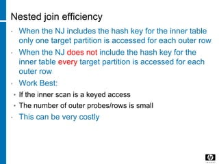
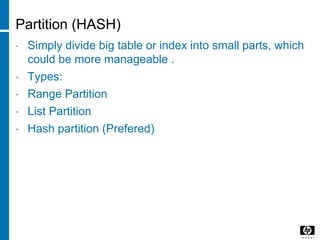
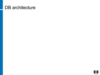
• SHOWSTATS FOR TABLE ACQ_SHIP_DTL_F ON
EVERY COLUMN
49 [Rev. # or date] – HP Restricted

50. Skew analysis: MaxF-based
• Maximum frequency (MaxF) for a column(s)
− frequency of the most popular value of the column(s) in the table
• A non-skewed partition key should satisfy
− MaxF(part-key) < 10% x (table rows out / number of partitions)
• Example
EDW_DEV.ACQ_SHIP_DTL_F is clustered by
(SHIP_ID,SHIP_DT,SHIP_LN_ITM_ID,SRC_SYS_KY,EFF_FRM_GMT_T
S )
T row rows out is 800M rows, with 128 partitions
Threshold = 10% x (1392671 / 128) = 1088 rows
MaxF(SHIP_ID) = 323 rows
MaxF(SHIP_DT) = 3095 rows
Non-skewed partitioning key is (SHIP_ID)

51. Checking skew
• View the histogram intervals table for a quick indication
− Fast, because only the histogram tables are accessed
− Requires a query, or a tool, to read the proper data
• New tool: “showstats”
− May not be precise, esp if stats are old/missing
• Doing “select-counts” for column of interest on actual table
− Precise, but may take a while to complete
− Uses system resources
• Combine both methods
− Use histograms to evaluate potential problems
− Use actual counts to verify

52. How to check Data Skew in HPDM?
52 [Rev. # or date] – HP Restricted

53. © 2008 Hewlett-Packard Development Company, L.P.
The information contained herein is subject to change without notice
DB/Server
architecture :
general/Shared
everything/Shared
nothing vs
SMP/NUMA/MPP

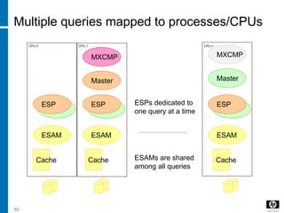
54. Common Server Architectures
• SMP: Symmetric Multi-Processor
• NUMA: Non-Uniform Memory Access
• MPP: Massive Parallel Processing
54 [Rev. # or date] – HP Restricted

55. SMP
• SHARE
55 [Rev. # or date] – HP Restricted
CPUs
Memory
controller
Memory
Bus
Front Side
Bus

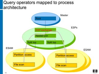
56. NUMA
56 [Rev. # or date] – HP Restricted
CPU
I/O
Memory Controller
Local Memory
Controller
Memory
CPU
I/O
Memory Controller
Local Memory
Controller
Memory
I/O
Local Memory
Controller
Memory
CPUMemory Controller
I/O
Local Memory
Controller
Memory
CPUMemory Controller
NUMA
Interconnectio
n Module

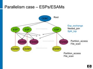
57. MPP
57 [Rev. # or date] – HP Restricted
CPU
I/O
Memory Controller
Local Memory
Controller
Memory
CPU
I/O
Memory Controller
Local Memory
Controller
Memory
I/O
Local Memory
Controller
Memory
CPUMemory Controller
I/O
Local Memory
Controller
Memory
CPUMemory Controller
MPP
Node Network

58. DB architecture

59. © 2008 Hewlett-Packard Development Company, L.P.
The information contained herein is subject to change without notice
Neoview Architecture - Software
HP Restricted [edit or delete]

60. Neoview Software
Feature Neoview
Operation System NonStop OS
Kernel Services NonStop Kernel(NSK)
Inter Process Comm. NonStop Kernel(NSK)
Clustering Services NonStop Kernel(NSK)
Disk Access Manager NonStop DP2
Transaction Manager NonStop TMF
ODBC/JDBC/ADO.net
Connectivity
Neoview Dataase
Connectivity
Services(NDCS)
Security Model NonStop Safeguard
LDAP security
Data Loader/Extractor Neoview
Transporter(NVT)

61. Neoview Hardware
Feature Neoview
Processor
Type
2 X Intel TM Itanium 9100
Series, dual-core,
1.66G/18M, 24GB
memory
Interconnect for
Processors
HP ServetNet
Interconnect Storage HP ServetNet
External
Communication
Ethernet 1Gb
Servers BL8610c blade(full height)
c-Class 7000 blade
enclosure
Storage Adapters/HBA NonStop CLIM subsystem
and adapters
Stroage Swithes SWD Fibre Channel Disk
Modules(FCDM)
Stroage Disks SWD MSA70 2.5’’ SAS

62. Built from industry-standard components for better
value
Switch
fabric
HP
StorageWorks
Fibre Channel
disks
GigabitEthernet
HP Integrity
servers
HP ServerNet
technology
….
….
BIclientETLclients
NDCS/ODBC/JD
BC/ADO.net
NonStop
OS/Database
Data Stroage
NonStop DP2/TMF(ESAM)

63. Neoview multi-segment architecture
• Active dual fault tolerant fabrics
• Multi-layered clustering (>128p)
• 500 MB/sec dedicated links
• Each segment adds bandwidth
• Cross sectional bandwidth up to
128 GB/sec
FT Clustered Mesh Fabric 1 to 16 segments
Neoview Segment Neoview Segment
Neoview Segment Neoview Segment

64. Unrivaled availability
Neoview failure protection
PS PSCS CS
X Fabric Y Fabric
P01 P14
M15 M28
M01 M14
P15 P28
P29 P42
M29 M42
P04
M04
RAID1 disk
failure protection
Controller failure
protection
Fabric failure
protection
Node 1 Node 2 Node 3 Node 4 Node 5 Node 6 Node 7 Node 8 Node 9 Node 10 Node 11 Node 12 Node 13 Node 14 Node 15 Node 16
BladeBlade
P01,P02 P03,P04 P19,P20P07,P08 P09,P10 P11,P12 P13,P14P05 P06 P21,P22P15,P16 P17,P18 P23,P24 P25,P26 P27,P28 P29,P30 P31,P32
B27,B30 B05 B28 B12,B21B02,B32 B03 B06 B04,B13 B07,B09B01,B31 B15,B17B08,B10 B11,B14 B16,B18 B19,B22 B20,B29 B23,B25 B24,B26
Primary
ESAM
Backup
ESAM
ESAM process
pair takeover
NDCS X
NDCS
reconnection
NDCS X, Y
NDCS Y
Query (ESP)
Abort/Resubmit
ESP X,
Y
ESP X ESP X

65. Question- What is configuration of our server?
• LED
- 8 segments/128 CPUs/each have 8G memory/two
disks(RAID1)
• IRN
- 16 segments/256 CPUs/each have 8G memory/two
disks(RAID1)
• GLD/SVR/PLT
- 16 segments/256 CPUs/each have 12G memory/pre
600G/two disks(RAID1)/294 TB
• MRC/TTN
- 32 segments/512 CPUs/CPUs/each have 12G memory/pre
600G/two disks(RAID1)/1.14PB

66. Unrivaled availability
Elimination of planned downtime
• Active and real-time database
loading
• Online database maintenance
• Create and populate index
• Create and refresh materialized
views
• Database reorganization
• Redistribute database (planned)
• Online schema evolution (planned)
• Online database and log
backup for recovery
• Removal Media Disaster
Recovery
Updates
Audit logs

67. • Shared-nothing MPP
− Each processor a unit of parallel work
• Database virtualization
− Data transparently hashed across all disks
• Parallel query execution
− Queries divided into subtasks and executed in
parallel with results streamed through memory
• Real-time data warehousing
− Mixed workload & transactional heritage
• Unrivaled availability
− Continuously available in spite of any single
point failure; online database operations
• Extreme processing power
− 1 Intel® Itanium® processor to 2 RAID 1
volumes
Architected for availability, scalability, and
performance
BIclientETLclients

68. Agenda
• EDW Architecture
• Neoview Architecture - Hardware
• Neoview Architecture - Software
• Neoview Client Tools

69. 69
Process architecture for a query
MXOSRVR – JDBC/ODBC server (aka: Master Executor, NDCS, Connect)
• Process to which a user connects
• Controls overall query execution
• Separate server is dedicated to each user connection
MXCMP – SQL compiler
• Separate compiler dedicated to each JDBC/ODBC server
• Generates query execution plan (operator tree) for a query
• Caches SQL plans for reuse
MXESP – Executor Server Process (ESP)
• “Helper” processes used for parallel execution of a query
• Can be many ESPs per query
• No more than 1 ESP per CPU per plan step (possibly less with Adaptive Segmentation)
• Dedicated to an active connection (JDBC/ODBC server), available for reuse
Encapsulated SQL Access Manager (ESAM) – (aka: Disk process, DP2/DAM)
• One logical* ESAM per disk volume
• Manages access to data for the volume (cache, locks, I/O etc.)
• Shared among all active queries – never dedicated
*implemented as a set of processes per disk volume

70. NDCS
• Neoview Database Connectivity Services
• NDCS and SQL processes involved in the
execution of SQL queries:
– NDCS Connection manager (MXOAS)
– NDCS Master process (MXOSRVR)
– SQL compiler (MXCMP)
– SQL ESPs (MXESP)
• DDL operations (including update statistics)
statement
– Processed by a second SQL compiler
– And when needed, ESPs

71. Connection & SQL execution flow
$MXOAS
NDCS
server CMP1client
(1)
Connection
request
(1) Create/assign to
NDCS Server
(2) SQL Statement (3) Compile
Statement
CMP2
CMP2
ESPs
CMP2
CMP2
ESAMs
1. Connection assigned to an NDCS Server
2. SQL statements sent to NDCS Server
3. SQL statement compiled
4. NDCS sends SQL plans to ESPs (“fix-up”)
5. Execution by NDCS and ESPs
6. ESAMs access/manage data
ESPs are helper processes used
for additional parallelism and to
perform other operations.
May not be used for all queries.
(4) “fix-up”,
send the plans
for the query
(5) (5)
(6)

72. SQL execution flow when doing DDL operation
NDCS
server CMP1
(1) Compile
Statement
CMP2
CMP2
ESP1s
• DDL statement passed to first compiler
• First compiler starts second compiler and additional ESPs (if needed)
• Second compiler does the work for the DDL operation
CMP2
CMP2
CMP2
ESP2s
(3) Executes DDL
statement
(2)
(2)

73. Process architecture for a query
• WMS – Workload Management Services
• Control/manage the use of key system resources
– CPU, memory
– Queues or executes queries based on resource availability
• Support workload services
– Configuration options for different workloads
• Time of day availability, priority, resource thresholds, rules, etc.
• Rules-based controls
– Connection: Service mapping based on client, application,
Role, etc.
– Compilation: Reject, hold, execute – based on compilation
metrics
– Execution rules: Can cancel or execute – based on run-time
metrics & comparison
• Collect and manage query run-time statistics (RTS)

74. WMS
• The Neoview Workload Management Services (WMS)
feature provides the infrastructure to help you manage
system resources in a mixed workload environment of
a Neoview platform. Using WMS, you can influence
when queries run and how many system resources
they are allowed to consume by assigning groups of
queries (that is, query workloads) to services.

75. AS Architecture (with WMS)
NDCS Server Components
(NEO System)
ODBC/JD
BC Client
WMS Server Componen
(NEO System)
1. Application prepares query
2. Server requests prepare of query
3. MXCMP compiles query
4. Server returns Success to application
5. Application requests execute of query
6. Server requests WMS for execution
7. WMS allows server to execute, returns
Affinity Value
8. Server requests execute of query with given
Affinity Value
9. Executor executes query
10. Server requests release of affinity value
11. Server returns success to application
System InfoRTS
1
Application Driver
5
4
6
7
WMS
10
2
MXCMP
3
NDCS
Server
EXE
8
9
11

76. ESP
• Executor Server Process
• Processes that communicate with the master (root server)
process
• Also, processes needed for intermediate steps –
repartitioning data, group bys, aggregation, etc.
• At Neoview this is MXESP process(its parent is the
MXOSRVR process which controls your sessions; and
MXCMP is the complier process)
• Simplistic query plans involve direct communications
between the CONNECT process and the ESAMs hosting
the data needed to fullfill the query access plan.

77. ESP
• For more complex queries involving complex operations, such as
repartitioned hash joins, and so on. The plan may be divided into
subtasks that are relegated to executive server process (ESPs) or even
layers of ESPs for parallel execution.
• ESP management is automatically controlled by the Neoview platform,
providing balanced processor utilization and accelerating query
performance.
• An aggregate operator possibly executed on ESAM or ESP base on
optimizer’s select, optimizer make this decision base on a lot of factor,
like using histogram statistics to estimate the rows out of row between
two operator compare with hash join vs. nested join, Or using histogram
statistics to predict whether the result set will too large to all fill in
memory or not. If result set is small it will use ESAM. Otherwise it will
use ESP.
• a Join operator will be done in ESP.

78. ESAM architecture – a closer look
• Each mirrored volume encapsulated
by an ESAM
• 2 ESAMs per processor
• Multiple ESAM threads
• Common I/O request queue
• Distributed data cache, lock pool, audit
buffer, SQL buffer
• I/O control
• Push-down SQL processing
• Mixed-workload management
– CPU,I/O requests & I/O accesses
Neoview platform
Processor
Processor n
ESAM
Request queue
I/O
transfers
to/from
disk
Data
cache
Lock
pool
Audit
buffer
Sqlmx
buffer

79. Prioritized mixed workload support
Prioritized SQL I/O
• Assigned by Workload
Management Services based
on service level the query
maps to
• Prioritizes I/O requests for
ESAM and processor execution
• Anti-starvation algorithm to
process low-priority work
Benefits
• Superior mixed workload
support
• Service level agreement
fulfillment
• Allows concurrent load,
maintenance and operational,
strategic/tactical, and analytical
query processing 79
Query
Low
Query
Medium
Queue
Cache
ESAM
….
Cache
ESAM
Cache
ESAM
Queue Queue
Processororsegmentboundary
Primary &
RAID 1 pair
Primary &
RAID 1 pair
Primary &
RAID 1 pair
LDV 1 LDV
2
LDV n
Query
High
Low Low Low
Medium MediumMedium
High HighHighLow Low Low
Medium MediumMedium
High HighHigh

80. Glance at HPDM

81. Glance at HPDM - Data Source

82. Glance at HPDM – Data Source

83. WMS
NDCS Connection
Manager(MXOSA)
CMP
Master
Executor
ESP
ESAM
Node 1 Node 2 Node 3 Node 4 ... Node n
...
...
ODBC/JDBC Client
TCP/IP
NDCS
server
CMP
NDCS
server
ESAM
LDV3
ESPESP ESP ESP
Cache
LDV3
LDV4
LDV4
LDVn
LDVn
LDV1
LDV1
LDV2
LDV2
ESAM
ESAM
ESAM
ESAM
ESAM
ESAM
ESAM
ESAM
Cache Cache Cache Cache
Neoview general Process

84. Query with ESPs mapped to processes/CPUs
Master
Cache Cache Cache
MXCMP
ESAMESAM ESAM
ESP ESPESP
CPU 0 CPU nCPU 1
84
May use multiple
layers of ESPs
3 process types executing query

85. ESP ESPESP
Multiple queries mapped to processes/CPUs
Master
ESAMESAM ESAM
Cache Cache Cache
MXCMP
ESP ESPESP
Master
MXCMP
CPU 0 CPU 1 CPU n
ESAMs are shared
among all queries
ESPs dedicated to
one query at a time
85

86. Query operators mapped to process
architecture
Root
Nested join
Partition access
File scan File scan
Partition access
Split top
Master
ESAM
ESAM
ESP exchange
ESPs
86
Split top

87. Parallelism case – ESPs/ESAMs
ODBC
Esp_exchange
Nested_join
Split_top
ESPESP ESP
ESAM1ESAM1 ESAM1
Partition_access
File_scan
ESAM2ESAM2 ESAM2 Partition_access
File_scan
Root