This document provides an overview of basic tools and concepts for storm chasing and severe weather forecasting, including:
1) Surface weather maps, radar/satellite images, upper air maps, and computer model forecasts are the primary tools used to analyze conditions and predict severe weather.
2) Key elements on surface maps include temperature, dew point, wind speed/direction, and fronts/boundaries separating air masses.
3) Upper air maps show pressure, winds, and features like troughs and ridges that influence surface weather patterns.
4) Computer models like the GFS, NAM, and RUC provide forecast guidance out to days in advance but have limitations and require experience to interpret.
This document discusses the procedures and tools used in weather forecasting. It describes how weather data is collected from over 9,500 observation stations and 7,400 ships worldwide and transmitted to analysis centers. Forecasts are made using synoptic charts, computer modeling, and satellite imagery from geosynchronous and low-Earth orbiting satellites. Forecasts can be short-range up to 48 hours, medium-range from 3 days to 3 weeks, or long-range from 2 weeks to a season. The goal of weather forecasting is to continue advancing techniques to better predict high-impact weather events.
Weather forecasting has evolved significantly over thousands of years from early observational methods to modern computer-based modeling. Early forecasting relied on patterns observed over generations, while today satellites and sensors collect global data that feeds complex models. Forecasting accuracy has improved markedly, though challenges remain as forecasts range further in time due to the chaotic nature of the atmosphere. Continued advances in computing power, data collection, and scientific understanding aim to further refine predictions.
5 - K Prasad - Weather forecasting in modern age-Sep-16indiawrm
Numerical weather prediction models have greatly improved forecasting accuracy through increased computing power, enhanced observational data from satellites and other sources, and more advanced modeling techniques. Global models run by organizations like NOAA provide short, medium, and extended forecasts of weather parameters on grids as fine as 20-25km. Regional models run at finer resolutions. Observational data is collected through a global network and transmitted via telecommunication systems to processing centers, which generate forecast products available in real-time.
The document discusses how weather is observed and measured through various instruments and technologies. It explains that weather refers to atmospheric conditions at a specific time and place, while climate deals with long-term patterns. It then describes how common weather elements like temperature, pressure, wind, moisture, clouds, and precipitation are defined and measured. The document outlines how weather data is represented in station models and weather maps. It concludes by noting how observation has advanced with radar and satellite imagery.
Progress and Challenges for the Use of Deep Learning to Improve Weather Forec...inside-BigData.com
In this deck from the UK HPC Conference, Peter Dueben from ECMWF presents: Progress and Challenges for the Use of Deep Learning to Improve Weather Forecasts.
"I will present recent studies that use deep learning to learn the equations of motion of the atmosphere, to emulate model components of weather forecast models and to enhance usability of weather forecasts. I will than talk about the main challenges for the application of deep learning in cutting-edge weather forecasts and suggest approaches to improve usability in the future."
Watch the video: https://wp.me/p3RLHQ-l1X
Learn more: https://www.ecmwf.int/
and
http://hpcadvisorycouncil.com/events/2019/uk-conference/agenda.php
Sign up for our insideHPC Newsletter: http://insidehpc.com/newsletter
Weather prediction technology is a global, big data enterprise. This talk will describe the huge quantities of information that make modern weather prediction possible, from satellite and radar data to surface observations and the output from numerical weather prediction models. The role of smartphones and other mobile devices for distributing forecasts and weather information will be discussed and the future of weather prediction will be outlined.
The document provides information about weather maps and weather concepts. It discusses key elements of weather maps including isobars, pressure cells, wind direction and speed. It explains that high pressure cells bring clear skies while low pressure cells bring cloud and rain. It also summarizes different types of rainfall including convectional, orographic and frontal rainfall. Seasons are determined by the positioning of pressure systems with lows over northern Australia in summer and highs in winter.
An Investigation of Weather Forecasting using Machine Learning TechniquesDr. Amarjeet Singh
1. The document discusses using machine learning techniques to forecast weather based on recorded data from weather stations.
2. It investigates using supervised learning algorithms like regression to predict future weather conditions based on historical data.
3. The models can provide short-term weather forecasts more quickly and using fewer resources than traditional complex physics models run on high-performance computing systems.
This document discusses how weather is observed and measured. It explains that weather refers to atmospheric conditions at a specific place and time, while climate deals with long-term patterns. It then describes the key variables that are measured, including temperature, pressure, wind, moisture, clouds, and precipitation. Common instruments for observing each variable are presented, as well as how weather data is represented in station models. The document concludes by noting the importance of upper-air and remote sensing data from weather balloons, satellites, and radar.
The document discusses the history of weather prediction and mapping from early folklore and weather logs to modern techniques. Key developments include the telegraph enabling rapid data sharing, radiosondes and dropsondes allowing upper-atmosphere measurement, and computers making complex calculations feasible. Richardson pioneered mathematical weather prediction using a grid-based "finite difference" technique to anticipate atmospheric motion.
The document discusses weather forecasting. It describes the process of forecasting as involving observation, collection and transmission of weather data, plotting and analysis of this data, and then analysis of weather maps and other tools to formulate a forecast. Key tools used in forecasting include weather maps, satellite and radar images, and numerical weather prediction models. The accuracy of forecasts depends on knowledge of weather conditions over a wide area.
Use of satellite imageries in weather forecastingDK27497
Satellite imagery provides valuable data for weather forecasting. Meteorologists use satellite images, which act as "eyes in the sky", to observe the atmosphere and track events like the formation of clouds. Different types of satellites like geostationary and polar-orbiting satellites provide imagery at varying resolutions, frequencies, wavelengths, and angles. Weather forecasting involves collecting data from stations, analyzing patterns in satellite images and charts, and issuing forecasts. Satellite images allow forecasters to predict conditions and natural hazards. Continued technological advances will further improve forecasting accuracy.
The document discusses various aspects of weather forecasting by the National Weather Service and U.S. Navy. It describes the different types of forecasts produced, including area forecasts by major Navy units, flight forecasts for successive flight stages, and local forecasts by ships and stations. It also outlines the roles of organizations like the National Oceanic and Atmospheric Administration, National Weather Service, and Navy Meteorology and Oceanography Command in coordinating weather data collection and forecasting activities.
Ch 14. weather forecasting ( application of data logging)Khan Yousafzai
Traditional weather forecasting relied on collecting data from various locations and recording it manually, which risked human error. Now, automated data logging uses sensors to regularly collect weather measurements like temperature, wind, and humidity without human intervention. This data is converted into a digital format and stored to improve accuracy of forecasts. Data logging allows for frequent, round-the-clock collection of weather data from remote locations.
The density and distribution of climatological stations to be established in a land network within a given area depend on the meteorological elements to be observed, the topography and land use in the area, and the requirements for information about the specific climatic elements concerned. This module highlights all these aspects.
Presentation of Weather It Is WRF forecast model results for temperature, precipitation, winds, and hurricane track and intensity. Given at the 8th WRF Users\' Workshop, Nat\'l Center. for Atmospheric Research, Boulder, Colorado, June 2008.
Atmospheric Dispersion in Nuclear Power Plant SitingHussain Majid
This document discusses atmospheric dispersion modeling for nuclear power plant siting. Meteorological data collection is important for modeling radioactive releases from plants during normal operation and accidents. Stability classes are determined from factors like temperature lapse rate, wind fluctuations, insolation, and cloud cover to characterize turbulence levels affecting dispersion. Both simple and complex terrain features must be considered when collecting and interpreting meteorological data used in dispersion calculations.
This document defines key weather vocabulary words including weather, atmosphere, temperature, front, wind, anemometer, meteorologist, and weather map. It provides short definitions for each term - weather is defined as the happenings in the atmosphere at a certain time, atmosphere as the air that surrounds Earth, and so on. A meteorologist is described as a scientist who studies weather and the atmosphere.
History of meteorology and invention of weather instrumentsIzzah Omaña
This document discusses the history of the development of meteorology and the invention of various weather instruments. It describes how early weather observation was based on sky observations, and how instruments like the barometer, thermometer, and hygrometer were later invented to measure air pressure, temperature, and humidity. It then discusses the development of weather mapping, satellites, and modern forecasting techniques using data from worldwide observation stations.
This document discusses weather forecasting and understanding weather maps. It explains that weather maps show isobars which indicate wind patterns around high and low pressure systems. Closer isobars mean stronger winds. It describes features of high and low pressure systems including wind direction. Cold fronts are shown where cold air pushes warm air upwards, potentially causing rain. Mechanisms that can trigger rain include fronts, low pressure systems, hills and turbulence. Clouds alone do not guarantee rain as clouds need sufficient moisture and lifting of air to produce meaningful rainfall.
Meteorologists gather weather data from surface stations and upper-level instruments to make accurate forecasts. Surface data is collected by the Automated Surface Observing System (ASOS) using instruments like thermometers, barometers, anemometers, hygrometers, ceilometers, and rain gauges to measure temperature, air pressure, wind, humidity, cloud height, and precipitation hourly at over 967 stations across the US. Upper-level data is obtained using radiosondes, weather radars, and satellites which can detect conditions in the troposphere and provide visible and infrared images of cloud cover. This information is needed to understand changes occurring in the atmosphere.
Radio waves are emitted from radar and bounce off clouds and objects to be recorded, allowing meteorologists to track wind speeds. Weather satellites record visible light, infrared light, and thermal data to track clouds, fires, pollution, auroras, and more. Surface weather maps depict isobars (lines of equal pressure), pressure fronts, precipitation, and use station models to show cloud cover, wind speed and direction, temperature, dew point, and barometric pressure changes. Computer programs analyze data and create forecast models to predict weather percentages and chances of precipitation for the next few days.
The history of meteorology began with simple observations of the sky mentioned in the Bible. The invention of instruments like the barometer and thermometer in the 1600s-1700s allowed for accurate measurement of weather conditions. Meteorology developed as a field in the 19th century with routine weather observations and transmission of data via telegraph. Theories of air masses and fronts were formulated in the 1920s. After World War II, technologies like weather radar and satellites revolutionized forecasting. Today, meteorology utilizes diverse instruments across spatial scales to study the atmosphere.
This document defines and describes several key atmospheric variables:
- Air temperature is measured with a thermometer in degrees Celsius, Fahrenheit, or Kelvin and shown on weather maps with isotherms. Solar radiation is the main source of heat for the atmosphere.
- Air pressure is measured with a barometer in units like millibars and shown on maps with isobars. Pressure is affected by altitude, temperature, and moisture and influences wind speed.
- Moisture in the air is measured with instruments like a hygrometer and shown as dew point temperature or relative humidity on station models. Dew point is the temperature at which air becomes saturated.
This document defines and explains key terms related to weather including: weather, atmosphere, temperature, front, wind, anemometer, meteorologist, and weather map. It provides brief definitions for each term, describing weather as happenings in the atmosphere, atmosphere as the air surrounding Earth, temperature as a measure of hot or cold, front as where two air masses of different temperatures meet, wind as the movement of air, anemometer as an instrument that measures wind speed, meteorologist as scientists who study weather and atmosphere, and weather map as a map showing weather data over a large area.
Meteorologists use tools like thermometers, anemometers, hygrometers, weather vanes, and barometers to measure temperature, wind speed, humidity, wind direction, and air pressure in order to study and predict weather patterns. They observe cloud conditions and types like cumulus, cirrus, stratus, and cumulonimbus clouds which can indicate different weather. Air mass movements and interactions at fronts where different air masses meet are responsible for most weather changes.
Why Machine Learning?
• Develop systems that can automatically adapt and customize
themselves to individual users.
– ...Why now?
• Flood of available data (especially with the
advent of the Internet)
• Increasing computational power
• Growi...
The document provides a detailed weather forecast for the Tuzla Airfield region of Romania for August 19th, 2012. It analyzes synoptic maps and charts to determine weather conditions, including clear skies with no phenomena, surface visibility over 10km, temperatures from 18C to 26C, and offshore winds from the north of 0.6-0.9m waves with periodicities of 3.6 to 4.05 seconds. The forecast concludes with specifics on sunrise, sunset, moonrise, moonset and cloud coverage.
The document discusses weather terminology and forecasting. It defines terms like air mass, air pressure, fronts, and precipitation. It explains how weather data is collected through satellites, radars, and other tools. Forecasting is done by analyzing this data using weather maps and models. Different types of weather like cold fronts and high pressure systems are indicated with symbols on maps.
1) Satellites provide a new tool for monitoring extreme rainfall events globally, including over oceans where gauges are sparse.
2) Analysis of TRMM satellite data shows that the relationship between maximum rainfall and duration (the Jennings law) exhibits two slopes for short and long durations, unlike the single slope seen in gauge data.
3) Satellites allow identifying regions experiencing the most extreme rainfall over timescales from days to years, such as Vietnam, Northeast India, and Colombia's Pacific coast.
Weather satellites and how to read the signsKella Randolph
The document provides information about weather terms, weather maps, and weather forecasting. It defines terms like air mass, air pressure, cold fronts, and warm fronts. It describes how weather data is collected using radars and satellites like GOES and POES. Weather forecasting uses data from these satellites as well as tools like the Beaufort scale. Forecasts are aided by understanding symbols on weather maps that represent phenomena like precipitation and high and low pressure systems.
This document provides an overview of an introductory meteorology course. It discusses key weather elements like temperature, pressure, humidity and clouds. It also covers weather phenomena like storms, fronts and maps. Satellite images are used to view weather patterns. The document outlines different types of storms and careers in meteorology. Weather and climate are explored in how they impact our lives and environment.
This document provides an overview of weather and climate concepts. It discusses how weather is caused by differences in temperature and air pressure between locations. It also describes common weather phenomena and how weather is forecasted using various instruments and models. The document outlines different climate zones and variables that influence climate. It explains phenomena like El Niño and hurricanes and how climate change is impacting environments and societies.
This document discusses using high resolution maps and 3D reconstructions of the atmosphere to study meteorological phenomena. It outlines various remote sensing techniques and datasets that can be used, including synthetic aperture radar interferometry (InSAR) and GPS tomography. InSAR phase measurements contain contributions from topography, atmospheric water vapor, and surface deformation. The document explores how the atmospheric signal in InSAR data is related to the precipitable water vapor content integrated along the radar signal path. This information could help identify patterns in atmospheric dynamics and types of clouds.
General Atmospheric
Circulation
Unit 6b
General Circulation of the Atmosphere
• Single-cell model (Hadley, 1735)
• Assumes:
– non-rotating earth
– uniform surface
• Low Pressure at Equator (warm air rising)
• High Pressure at Poles (cold air sinking)
• Creates a thermal convection cell
Three Cell Model
• Due to earth’s rotation and other
dynamic factors there are typically 3
primary cells
– Hadley Cell (tropics)
– Midlatitude Cell (Ferrel)
– Polar Cell (polar zones)
Three Cell Model
Hadley Cell
Primary High & Low Pressure Areas
Equatorial Low Pressure (ITCZ)
Subtropical High Pressure
Subpolar Low Pressure
Polar High Pressure
Equatorial Low Pressure
Intertropical Convergence Zone (ITCZ)
±10° N & S
Thermally-induced low pressure
Clouds and rain
Limited wind (doldrums)
Seasonal shift N-S
Subtropical High Pressure
• Dynamic high pressure
– subsiding air of Hadley Cell
– between 20° - 35° N & S
• Creates hot, dry air
– Clear skies, limited wind (horse latitudes)
– e.g., Bermuda High, Hawaiian High
• Strengthen/weaken seasonally
• Shift N & S with sun’s declination
Subpolar Low Pressure
• Dynamic low pressure
– air forced to rise
– along polar front
• Cool, moist, cloudy
• Frequent cyclonic storms
– e.g., Aleutian Low, Icelandic Low
• strengthen/weaken seasonally
General Circulation
(Side-View)
General Circulation – Surface Winds
Trade Winds (tropical)
Westerlies (midlatitudes)
Polar Easterlies
Trade Winds
Trade Winds (tropical)
– from subtropical highs to equatorial lows
– northeast trades & southeast trades
Westerlies
Westerlies (midlatitudes)
– from the subtropical highs to the subpolar lows (west à
east)
– tend to be wavy (meridional flow)
Polar Easterlies
Polar Easterlies
– from polar highs to subpolar lows
– variable, cold, dry winds
www.atmo.arizona.edu
General Circulation – Upper Air Flow
(geostrophic winds)
• Westerlies
– subtropics à poles
– occur as Rossby Waves Jet Streams
– areas of high wind velocity within the westerlies
• Subtropical Jet
– 20° - 50° N & S
– 10,000 – 15,000 m
• Polar Jet
– 30° - 70° N & S
– 8,000 – 12,000 m
Jet Stream
Rossby Waves
http://svs.gsfc.nasa.gov/vis/a010000/a0
10900/a010902/
http://www.geography.hunter.cuny.edu/tbw/wc
.notes/7.circ.atm/rossby_waves.htm
Local and Regional Winds
Ocean Circulation
Unit 6c
Local and Regional Winds
Land/Sea Breeze
Mountain/Valley Breeze
Katabatic Winds
Compressional Winds
Monsoons
Land/Sea Breeze
• thermal circulation
• best developed in summer
• land heats up during day, creates relative low
pressure forming sea breeze
• land cools off at night creates relative high pressure
forming land breeze
Mountain/Valley Breeze
• thermal circulation
• best developed in summer
• slopes heat up during the day causing an upslope
wind (valley breeze)
• slopes cool off at night causing a downslope wind
(mountain breeze)
Katabatic Wind
Cold downslope wind
cold air = greater densit ...
This document discusses remote sensing and meteorology. It defines remote sensing as obtaining information about physical objects through non-contact sensors. Meteorology is the study of atmospheric phenomena like weather. Meteorological satellites and weather radars are important tools for monitoring weather. Satellites provide global coverage of cloud patterns and weather systems from space. They capture visible, infrared, and water vapor images to study cloud formations, temperatures, and moisture in the atmosphere. Radar emits microwaves that bounce off water droplets in clouds to measure precipitation and cloud locations. Satellite weather monitoring improves forecasts, especially over oceans with sparse weather station data.
A scatterometer is a microwave radar sensor used on satellites to measure ocean wind speed and direction by measuring the strength of radar signals reflected from the ocean surface. It consists of three subsystems: an electronics subsystem that generates and receives radar signals; an antenna subsystem that transmits signals and collects reflections; and a command and data subsystem that controls operations and processes data. Scatterometer data helps scientists study weather patterns, climate change, and unusual phenomena like El Niño by providing information about ocean winds.
This is the paper for our final project in our Numerical Weather Prediction class. For this project, we analyzed model output from a Nested Regional Climate Model (NRCM), which is an adaptation of the Advanced Research WRF (ARW). The model output variables analyzed were outgoing long wave radiation (OLR) and precipitation (convective plus non-convective). The goal of this research project was to determine why errors were occurring in the model, and what could be done to correct them. In this paper, we provide some insight into why these errors occurred, particularly errors within the model which equaled or surpassed the overall mean climate error.
This document discusses using geostationary satellites to predict aviation weather hazards like downbursts and fog. It describes how satellite measurements can be used to calculate indices like the Microburst Wind Potential Index (MWPI) to forecast downburst wind speeds up to 3 hours in advance. Case studies of downbursts in Southern California in 2014 and fog in Salt Lake City in 2015 are presented, showing how satellite data matched observations. The conclusions emphasize that MWPI has conditional skill in forecasting thunderstorm winds and that fog can be detected using infrared channel brightness temperature differences from GOES satellites.
1) The document evaluates high-resolution 5km weather forecasts in Thailand and nearby regions using the MM5 model and compares them to AMSU satellite observations of 79 tropical storm systems over one year.
2) The MM5 forecasts generally captured the morphology, intensity, and area of the storms observed by AMSU, though sometimes overestimated ice particle size and had location differences.
3) The forecasts provided useful information about tropical storms up to 8 hours in advance but could be improved with higher resolution data and a more accurate prediction model.
1) Advances in radar techniques have allowed for continuous observation of the Earth's atmosphere from the lower to upper atmosphere. 2) The latest techniques include active phased array radars like the MU radar in Japan which can rapidly scan beams to accurately measure wind velocity. 3) Atmospheric radars provide high resolution continuous data on winds and have revealed processes like gravity wave propagation, saturation and their influence on mean flows.
The document discusses various weather and climate concepts including:
- Weather is the current atmospheric conditions while climate is the average weather over time.
- High pressure systems are associated with clear skies and dry conditions while low pressure systems bring clouds and rain.
- Weather maps use lines of equal pressure (isobars) and symbols to show wind speed and direction helping predict future conditions.
This document provides information on a group assignment submitted by 16 students for their Introduction to Remote Sensing course. It includes the group number, course details, student names and registration numbers, and the assignment questions. The assignment involves describing the TRMM satellite's owner and location, orbital characteristics, identifying its onboard sensors and providing details on each sensor's specifications and functioning.
This study examines the effect of rain on ASCAT observations of sea surface radar cross-section using simultaneous rain measurements from NEXRAD radars. Three rain events were analyzed over Gulf of Mexico in 2008-2009. Results show rain can cause substantial increases in backscatter, from 2-4 dB depending on incidence angle, leading to errors in estimated wind speed of around 60%. The change in backscatter was found to depend on incidence angle but consequences were similar across angles due to wind speed models. Substantial wind errors were identified for rain rates of 6-20 mm/hr. Extra care is needed when using ASCAT data in tropical rainy regions.
This document summarizes research on measuring all-weather wind speeds using both passive microwave radiometers and active microwave scatterometers. It discusses the challenges of high wind speeds (>20 m/s) and winds in rain, and improvements made to wind retrieval algorithms. An improved Ku-band geophysical model function (GMF) for QuikSCAT was developed using WindSat winds for validation. Comparisons show WindSat provides more accurate winds than QuikSCAT in rain. The study concludes that while passive radiometers have strengths at high winds and in rain, scatterometers remain impacted without dual-frequency capabilities.
Similar to Davies 2011 chaser con forecast school slideshare (20)
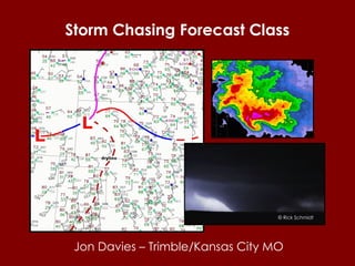
How to Fix the Import Error in the Odoo 17Celine George
An import error occurs when a program fails to import a module or library, disrupting its execution. In languages like Python, this issue arises when the specified module cannot be found or accessed, hindering the program's functionality. Resolving import errors is crucial for maintaining smooth software operation and uninterrupted development processes.
it describes the bony anatomy including the femoral head , acetabulum, labrum . also discusses the capsule , ligaments . muscle that act on the hip joint and the range of motion are outlined. factors affecting hip joint stability and weight transmission through the joint are summarized.
Thinking of getting a dog? Be aware that breeds like Pit Bulls, Rottweilers, and German Shepherds can be loyal and dangerous. Proper training and socialization are crucial to preventing aggressive behaviors. Ensure safety by understanding their needs and always supervising interactions. Stay safe, and enjoy your furry friends!
ISO/IEC 27001, ISO/IEC 42001, and GDPR: Best Practices for Implementation and...PECB
Denis is a dynamic and results-driven Chief Information Officer (CIO) with a distinguished career spanning information systems analysis and technical project management. With a proven track record of spearheading the design and delivery of cutting-edge Information Management solutions, he has consistently elevated business operations, streamlined reporting functions, and maximized process efficiency.
Certified as an ISO/IEC 27001: Information Security Management Systems (ISMS) Lead Implementer, Data Protection Officer, and Cyber Risks Analyst, Denis brings a heightened focus on data security, privacy, and cyber resilience to every endeavor.
His expertise extends across a diverse spectrum of reporting, database, and web development applications, underpinned by an exceptional grasp of data storage and virtualization technologies. His proficiency in application testing, database administration, and data cleansing ensures seamless execution of complex projects.
What sets Denis apart is his comprehensive understanding of Business and Systems Analysis technologies, honed through involvement in all phases of the Software Development Lifecycle (SDLC). From meticulous requirements gathering to precise analysis, innovative design, rigorous development, thorough testing, and successful implementation, he has consistently delivered exceptional results.
Throughout his career, he has taken on multifaceted roles, from leading technical project management teams to owning solutions that drive operational excellence. His conscientious and proactive approach is unwavering, whether he is working independently or collaboratively within a team. His ability to connect with colleagues on a personal level underscores his commitment to fostering a harmonious and productive workplace environment.
Date: May 29, 2024
Tags: Information Security, ISO/IEC 27001, ISO/IEC 42001, Artificial Intelligence, GDPR
-------------------------------------------------------------------------------
Find out more about ISO training and certification services
Training: ISO/IEC 27001 Information Security Management System - EN | PECB
ISO/IEC 42001 Artificial Intelligence Management System - EN | PECB
General Data Protection Regulation (GDPR) - Training Courses - EN | PECB
Webinars: https://pecb.com/webinars
Article: https://pecb.com/article
-------------------------------------------------------------------------------
For more information about PECB:
Website: https://pecb.com/
LinkedIn: https://www.linkedin.com/company/pecb/
Facebook: https://www.facebook.com/PECBInternational/
Slideshare: http://www.slideshare.net/PECBCERTIFICATION
How to Manage Your Lost Opportunities in Odoo 17 CRMCeline George
Odoo 17 CRM allows us to track why we lose sales opportunities with "Lost Reasons." This helps analyze our sales process and identify areas for improvement. Here's how to configure lost reasons in Odoo 17 CRM
বাংলাদেশের অর্থনৈতিক সমীক্ষা ২০২৪ [Bangladesh Economic Review 2024 Bangla.pdf] কম্পিউটার , ট্যাব ও স্মার্ট ফোন ভার্সন সহ সম্পূর্ণ বাংলা ই-বুক বা pdf বই " সুচিপত্র ...বুকমার্ক মেনু 🔖 ও হাইপার লিংক মেনু 📝👆 যুক্ত ..
আমাদের সবার জন্য খুব খুব গুরুত্বপূর্ণ একটি বই ..বিসিএস, ব্যাংক, ইউনিভার্সিটি ভর্তি ও যে কোন প্রতিযোগিতা মূলক পরীক্ষার জন্য এর খুব ইম্পরট্যান্ট একটি বিষয় ...তাছাড়া বাংলাদেশের সাম্প্রতিক যে কোন ডাটা বা তথ্য এই বইতে পাবেন ...
তাই একজন নাগরিক হিসাবে এই তথ্য গুলো আপনার জানা প্রয়োজন ...।
বিসিএস ও ব্যাংক এর লিখিত পরীক্ষা ...+এছাড়া মাধ্যমিক ও উচ্চমাধ্যমিকের স্টুডেন্টদের জন্য অনেক কাজে আসবে ...
Main Java[All of the Base Concepts}.docxadhitya5119
This is part 1 of my Java Learning Journey. This Contains Custom methods, classes, constructors, packages, multithreading , try- catch block, finally block and more.
A Strategic Approach: GenAI in EducationPeter Windle
Artificial Intelligence (AI) technologies such as Generative AI, Image Generators and Large Language Models have had a dramatic impact on teaching, learning and assessment over the past 18 months. The most immediate threat AI posed was to Academic Integrity with Higher Education Institutes (HEIs) focusing their efforts on combating the use of GenAI in assessment. Guidelines were developed for staff and students, policies put in place too. Innovative educators have forged paths in the use of Generative AI for teaching, learning and assessments leading to pockets of transformation springing up across HEIs, often with little or no top-down guidance, support or direction.
This Gasta posits a strategic approach to integrating AI into HEIs to prepare staff, students and the curriculum for an evolving world and workplace. We will highlight the advantages of working with these technologies beyond the realm of teaching, learning and assessment by considering prompt engineering skills, industry impact, curriculum changes, and the need for staff upskilling. In contrast, not engaging strategically with Generative AI poses risks, including falling behind peers, missed opportunities and failing to ensure our graduates remain employable. The rapid evolution of AI technologies necessitates a proactive and strategic approach if we are to remain relevant.
3. 74 62 051 Air pressure in millibars (upper right) (here 1005.1 mb) Temperature (upper left) (in o F on surface maps, here 74 o F ) Dew point (lower left) (a measure of moisture, in o F on surface maps, here 62 o F ) Wind direction and speed (here from the south-southwest at 15 knots) Line extending outward gives direction from which wind is blowing, barb gives speed in knots (kts): full barb = 10 kts; ½ barb = 5 kts (1 knot = 1.15 miles per hour) Basic surface station weather observation plot Current weather (middle left) (here, light rain) Station location
5. A dryline is a boundary between dry air to the west and moist air to the east. Moist air (high dew points) Dry air (low dew points) dryline
6.
7. Wind flow around low pressure is counterclockwise with air spiraling inward toward the center. Wind flow around high pressure is clockwise with air spreading outward from the center.
8.
9.
10. Older thunderstorms or clusters of storms can produce boundaries due to cool air flowing outward from some of the storms. These outflow boundaries can behave like small cold fronts, warm fronts or stationary fronts. outflow boundary from storms over southeast KS and southwest MO
11.
12. Satellite and radar information can help with weather map analysis. Radar Satellite
13.
14.
15.
16.
17.
18. This 500 mb map (~ 18,000 ft MSL) is the result of information from radiosondes:
19. Radiosondes released twice per day (6 a.m. CST and 6 p.m. CST) give us weather observations above the ground. Radiosonde : a box equipped with weather instruments and a radio transmitter attached to a gas-filled balloon. North American radiosonde sites
20. Weather maps above ground are important because they tell us a lot about what will be going on with our weather at the ground. Changes in the upper pressure and wind patterns and the jet stream help meteorologists to predict significant changes in our weather.
22. Jet stream (purple) (18,000-30,000 ft MSL) surface fronts Where jet stream winds and upper flow dip south, weather becomes colder Where jet stream winds and upper flow bulge north, weather becomes warmer Relationship of jet stream and upper winds to fronts trough ridge Surface fronts are usually located close to and beneath the jet stream !
23. The jet stream winds generally run along the tighter contours of weather maps at 500 mb (roughly 18,000 ft above sea level) and 300 mb (roughly 30,000 ft above sea level). These contours make troughs and ridges in the flow aloft that greatly affect our weather at the ground.
24. wind flow and contours at roughly 18,000 ft MSL (500 mb) general cloudiness & storminess (divergence aloft – winds spreading apart to create lift) less clouds & “nicer” weather (convergence aloft- winds pushing together to create sinking) Troughs and ridges are waves aloft … wave wave
25. Shortwaves (smaller waves of energy in the upper flow) move through the larger troughs and ridges (longwaves), generating more concentrated areas of clouds and storminess within the larger troughs and ridges.
26. Longwave trough 500 mb ~ 18,000 ft MSL Longwave ridge Longwave trough Shortwave Shortwave Shortwave
27. Longwave trough 500 mb ~ 18,000 ft MSL Longwave ridge Longwave trough Shortwave Shortwave rising motion (clouds & storms) rising motion (clouds & storms) Shortwave rising motion (clouds & storms) sinking motion (better weather) sinking motion (better weather) sinking Note the areas of weather just ahead of these waves aloft – these shortwaves “plow up” the atmosphere, so to speak, to create lift and storminess.
28. Fronts also tend to move with the stronger wave disturbances aloft in the jet stream. ? strong shortwave aloft strong shortwave aloft surface front surface front dryline 500 mb contours and surface systems (a spring storm)
29. 300 mb 500 mb surface 30,000 ft (9 km MSL) 18,000 ft (5.5 km MSL) Ground level L H L L H cold cold cold warm warm warm H H Upper air maps, different “slices” through the atmosphere at increasing elevations, help meteorologists understand and predict all this weather.
30. Tornadic supercells possible S or SE surface winds & sizable CAPE (instability) (warm air & large dew points) L Divergence Winds veer (become more westerly) and increase with height Jet stream and divergence aloft (winds spreading apart) with upper trough / wave Meteorological setting for possible supercells and tornadoes Ground level MSL (5.5 km) MSL (3.0 km) MSL (1.5 km) MSL (9.0 km)
31. Ground level L divergence Meteorological setting for possible supercells and tornadoes We’ll look mainly at these levels aloft. MSL (5.5 km) MSL (3.0 km) MSL (1.5 km) MSL (9.0 km) ‘ upper levels’ ‘ mid levels’ ‘ low levels’
32. Ground level L divergence Notice that the “ mb” numbers (850 – 700 – 500 - 300) get smaller with height, just the opposite of elevation . Meteorological setting for possible supercells and tornadoes MSL (5.5 km) MSL (3.0 km) MSL (1.5 km) MSL (9.0 km) ‘ upper levels’ ‘ mid levels’ ‘ low levels’
33. ~ 18,000 ft / 5.5 km MSL Eta/NAM/WRF model forecast from UCAR site
34. ~ 10,000 ft / 3.0 km MSL Eta/NAM/WRF model forecast from UCAR site
35. ~ 5,000 ft / 1.5 km MSL Eta/NAM/WRF model forecast from UCAR site
38. Computer model forecasts use current data observations to initialize numerical models that approximate the atmosphere’s behavior. These models are then “run” forward in time using a computer to solve physical equations to make a forecast.
39. GFS (Global Forecast System): goes out to 16 days (usually displayed only out to 7 or 10 days), run 4 times per day (the 12z morning & 00z evening runs are best!) NAM (North American Mesoscale): goes out to 3.5 days (84 hours), run 4 times per day (again, the 12z morning & 00z evening runs are best!) (also called the WRF or Eta) RUC (Rapid Update Cycle): goes out to 18 hours (usually displayed only out to 12 hours), run hourly. (The NAM & RUC have higher resolution and more detail) Here are the main computer models that are run and maintained by the National Weather Service (National Centers for Environmental Prediction, or NCEP) and used by most forecasters:
40. The GFS is used to look farther ahead (out to 2 weeks), but it is very unreliable beyond 5-7 days. The early panels can also be used as a comparison to the NAM. The NAM/WRF/Eta is used to look out to 3 days or so, and is more detailed than the GFS. The panels out to 12 hours can also be used as a comparison to the RUC. The RUC is used the day of an impending event and is updated frequently with available current observations for even more detail.
41. You can access output from these models at many internet sites… The UCAR site above has been around for a long time: www.rap.ucar.edu/weather
43. Some other sites with computer model forecast output: Earl Barker’s site: www.wxcaster.com/conus_0012_us_models.htm (NAM/WRF & GFS) www.wxcaster.com/conus_offhr_models.htm (RUC) College of DuPage: weather.cod.edu/forecast (RUC, NAM/WRF, & GFS) TwisterData: www.twisterdata.com (RUC, NAM/WRF, & GFS) Unisys Weather: weather.unisys.com (RUC, NAM/WRF & GFS)
44. Example of computer model output: 12 hr forecast NAM model CAPE (instability) UCAR site: www.rap.ucar.edu/weather/model
45. Example of computer model output: 12 hr forecast RUC model 3 hr accumulated precipitation Earl Barker’s site: www.wxcaster.com/conus_offhr_models.htm (RUC)
46. Example of computer model output: day 2 through day 10 forecast GFS 10 day 500 mb contours (colors) and surface isobars (black) Unisys site: weather.unisys.com
47. Example of computer model output: 180 hr forecast GFS 6 hr accumulation precipitation forecast at 7.5 days TwisterData site: www.twisterdata.com
48.
49. Part of the job of meteorologists making forecasts is to use their knowledge and experience to determine when model guidance is reasonably accurate and useful, and when it is not. Accepting computer model forecast output without question and thought is not really weather forecasting. True weather forecasting requires experience! However, one can make a quick “forecast guess” for a tornado chase by looking at only a few panels of model output. Just understand that is only a crude guide based on a computer’s “opinion”, rather than a true forecast.
50.
51. Then, subtract the proper number of hours for your time zone from the UTC time to get your local time in a 24-hr or “military” time system. UTC is Universal Time Coordinated, the same as Greenwich Mean Time (GMT) or Zulu time (Z). To convert from UTC time to local time: First, learn to think in a 24-hr time system (“military time”):
52. Pacific Time Zone: Subtract 8 hours from the UTC time to get PST time. Subtract 7 hours from the UTC time to get PDT time. Mountain Time Zone: Subtract 7 hours from the UTC time to get MST time. Subtract 6 hours from the UTC time to get MDT time. Central Time Zone: Subtract 6 hours from the UTC time to get CST time. Subtract 5 hours from the UTC time to get CDT time. Eastern Time Zone: Subtract 5 hours from the UTC time to get EST time. Subtract 4 hours from the UTC time to get EDT time. ST = Standard time DT = Daylight time
53.
54.
55. 0000 UTC = 6:00 p.m. CST = 7:00 p.m. CDT 0300 UTC = 9:00 p.m. CST = 10:00 p.m. CDT 0600 UTC = midnight CST = 1:00 a.m. CDT 0900 UTC = 3:00 a.m. CST = 4:00 a.m. CDT 1200 UTC = 6:00 a.m. CST = 7:00 a.m. CDT 1500 UTC = 9:00 a.m. CST = 10:00 a.m. CDT 1800 UTC = noon CST = 1:00 p.m. CDT 2100 UTC = 3:00 p.m. CST = 4:00 p.m. CDT Table converting Universal Time (UTC) to Central Time (CST or CDT): Or, if all this seems too complicated, you can memorize the time conversions for your specific time zone, and work from there:
56. Also, remember that dates change backwards a day when doing evening and early nighttime UTC time conversions. Above, 0000 UTC 5 May 2007 is actually 7:00 pm CDT 4 May 2007 and, 00 UTC 21 February 2011 is actually 6:00 pm CST 20 February 2011
57.
58.
59.
60. (CAPE) convective available potential energy Yellow area is where lifted low-level air parcels are warmer than their environment -- a “positive” area Large CAPE means the atmosphere is very unstable. Moisture profile Temperature profile SkewT-log p diagram – a thermodynamic diagram
61.
62.
63.
64.
65.
66. Wind at 6 km above ground (near 500 mb) (from SSW at 20 kts) Wind at ground level (from SSE at 15 kts) 0-6 km bulk shear is the straight-line vector difference between 2 vectors: the surface wind, and the wind at 6 km above ground. Wind at 6 km above ground (near 500 mb)(from SW at 47 kts) Wind at ground level (from SSE at 15 kts) Here, the 0-6 km bulk shear is only 7 kts ( very poor ) Here, the 0-6 km bulk shear is around 40 kts ( very good for supporting supercells)
71. 0-1 km SRH is a measure of low-level wind shear -- it measures the area under the wind profile “curve” below 1 km... The larger the curve, the larger the low-level wind shear. Winds at increasing 200 m intervals above ground up to 1 km (1000 m) (winds increase in speed & become more southwesterly with height) Wind at ground level (from SE at 15 kts) Wind at 1 km above ground (just below 850 mb) (from SW at 35 kts) Here, the 0-1 km SRH is around 210 m 2 /s 2 ( good enough when combined with 2000-2500 J/kg of CAPE or more to support low-level meoscyclones & possible tornadoes) This red line is a hodograph Good low-level wind profile for supercell tornadoes
72. 0-1 km SRH is a measure of low-level wind shear -- it measures the area under the wind profile “curve” below 1 km... The larger the curve, the larger the low-level wind shear. Winds at increasing 200 m intervals don’t increase in speed with height, and the wind profile is “small” with not much of a “curve” Wind at ground level (from SE at 15 kts) This red line is a hodograph Here, the 0-1 km SRH is only around 70 m 2 /s 2 ( very poor for supporting low-level meoscyclones & tornadoes) Poor low-level wind profile for supercell tornadoes Wind at 1 km above ground (just below 850 mb) (from SSW at 19 kts)
73. 5/13/09 NW Missouri (non-tornadic supercell) 5/13/09 NC Missouri (EF2 tornadic supercell) 0-1 km SRH from contrasting hodographs 0-1 SRH = 70 m 2 /s 2 0-1 SRH = 430 m 2 /s 2 poor very good
74.
75. Tilting and stretching of horizontal vorticity (low-level wind shear): Low-level mesocyclones, possible tornadoes? Combinations of CAPE and SRH are important for this process.
79. Divergence ahead of strong 500 mb trough -- spreading of winds causes upward motion to trigger storms
80. cooling with height cooling with height warming with height capping inversion moisture profile temperature profile SkewT-log p diagram – a thermodynamic diagram CAPE above capping inversion can’t be realized capping inversion is near 700 mb
81. March approx > 5-6 o C April approx > 7-8 o C May approx > 9-11 o C June approx > 12-13 o C August approx > 12 o C September approx > 9-11 o C October approx > 7-8 o C November approx > 5-6 o C 700 mb temperature estimations of areas that are “capped” (too warm aloft for thunderstorms): Spring Fall This chart doesn’t work well in the western High Plains due to elevation (e.g., eastern NM, eastern CO, far western NE, etc.).
82. Capping not an issue in this case (far south of target area) Storms initiating?
88. A word about storm motion… It’s important to get an idea of which direction and how fast mature storms and supercells will be moving on a given day. That way you can intercept more effectively, and also plan quickly to get out of the way when you have to. You can use the 500 mb winds to make a very rough storm motion estimate (about 1/2 to 2/3rds the 500 mb wind speed and slightly to the right of the direction). You can also find more specific storm motion estimates on some computer model sites, such as Twisterdata.
89.
90.
91.
92.
93.
94. Sig Tor Parameter (STP) incorporates CAPE, SRH, deep shear, & LCL height into one parameter Target?
96. Tornadic storm (EF3), much farther south than original target near front Non-tornadic storms well north of surface stationary front Real observations…
99. Here’s another case comparing model output, This time starting a little farther out in time (48 hrs), and then moving on up to making target adjustments during the day of the actual chase…
100.
101.
102. 48-hr “radar echo forecast” from NAM model (Earl Barker’s NAM site)
103.
104. From this and surface map forecasts, warm front does not move as far north as on earlier 48-hr forecasts
105. 12-hr “radar echo forecast” from NAM model (Earl Barker’s NAM site) Target a little farther south?
109. March approx > 5-6 o C April approx > 7-8 o C May approx > 9-11 o C June approx > 12-13 o C August approx > 12 o C September approx > 9-11 o C October approx > 7-8 o C November approx > 5-6 o C 700 mb temperature estimations of areas that are “capped” (too warm aloft for thunderstorms): Spring Fall This chart doesn’t work well in the western High Plains due to elevation (e.g., eastern NM, eastern CO, far western NE, etc.).
110. Note “cap” estimate from chart – storms did not build much south of OK/TX border
111.
112.
113.
114. Many storm chasers who are good forecasters often have an intuitive sense about where to target after looking over data. If you feel you have that, try not to let “too much knowledge” cause you to over think chase target decisions. Try to stay in touch with your “gut feelings”, and use the knowledge you learn to supplement and confirm your intuitive sense about potential chase settings. .